HAL Id: hal-00318251
https://hal.archives-ouvertes.fr/hal-00318251
Submitted on 1 Feb 2007
HAL is a multi-disciplinary open access
archive for the deposit and dissemination of
sci-entific research documents, whether they are
pub-lished or not. The documents may come from
teaching and research institutions in France or
abroad, or from public or private research centers.
L’archive ouverte pluridisciplinaire HAL, est
destinée au dépôt et à la diffusion de documents
scientifiques de niveau recherche, publiés ou non,
émanant des établissements d’enseignement et de
recherche français ou étrangers, des laboratoires
publics ou privés.
Upper altitude limit for Rayleigh lidar
P. S. Argall
To cite this version:
P. S. Argall. Upper altitude limit for Rayleigh lidar. Annales Geophysicae, European Geosciences
Union, 2007, 25 (1), pp.19-25. �hal-00318251�
www.ann-geophys.net/25/19/2007/ © European Geosciences Union 2007
Annales
Geophysicae
Upper altitude limit for Rayleigh lidar
P. S. Argall
Dept. of Physics and Astronomy, The University of Western Ontario, London, Ontario, Canada
Received: 17 October 2006 – Revised: 4 January 2007 – Accepted: 15 January 2007 – Published: 1 February 2007
Abstract. It has long been assumed that Rayleigh lidar can be used to measure atmospheric temperature profiles up to about 90 or 100 km and that above this region the technique becomes invalid due to changes in atmospheric composition which affect basic assumptions on which Rayleigh lidar is based. Modern powerful Rayleigh lidars are able to mea-sure backscatter from well above 100 km requiring a closer examination of the effects of the changing atmospheric com-position on derived Rayleigh lidar temperature profiles.
The NRLMSISE-00 model has been used to simulate lidar signal (photon-count) profiles, taking into account the effects of changing atmospheric composition, enabling a quantita-tive analysis of the biases and errors associated with extend-ing Rayleigh lidar temperature measurements above 100 km. The biases associated with applying a nominal correction for the change in atmospheric composition with altitude has also been investigated.
The simulations reported here show that in practice the up-per altitude limit for Rayleigh lidar is imposed more by the accuracy of the temperature or pressure used to seed the tem-perature retrieval algorithm than by accurate knowledge of the atmospheric composition as has long been assumed. Keywords. Atmospheric composition and structure (Pres-sure, density, and temperature; Transmission and scattering of radiation; Instruments and techniques)
1 Introduction
Rayleigh lidar is a well established technique used to de-termine atmospheric temperature profiles from the mid-stratosphere (∼30 km) to the lower thermosphere (∼95 km), (Chanin, 1984; Sica et al., 1995).
Correspondence to: P. S. Argall
Rayleigh lidars measure the intensity of light backscat-tered by the atmosphere, as a function of altitude, from a pulsed laser. The measured intensity profile is often called a photon-count (or photocount) profile as, in practice; the in-tensity is measured by counting photons.
Several algorithms have been suggested which allow the determination of a temperature profile from a measured photon-count profile (Hauchecorne and Chanin, 1980, Shi-bata et al., 1986; Gardner et al., 1989). These algorithms are all based on the same physical principals and make the following two basic assumptions:
1. the atmosphere behaves like an ideal gas, and 2. the atmosphere is in hydrostatic equilibrium.
The algorithm used in this work explicitly determines a rel-ative pressure profile from the relrel-ative mass-density profile, which is determined from the photon-count profile. The rela-tive pressure and mass-density profiles are used to determine an absolute temperature profile. The first of the two above assumptions is used in the determination of the relative pres-sure profile from the relative mass-density profile. The sec-ond assumption is used in the calculation of the temperature profile from the relative mass-density and pressure profiles.
Early in the development of the Rayleigh lidar technique it was recognised that there was an upper altitude limit for the application of this technique (Kent and Wright, 1970) due to the changing composition of the atmosphere above about 90 km. This limit has been informally extended to about 100 km over the past few decades as our understand-ing of this region of the atmosphere has improved. However this limit has remained vague and the effects of extending Rayleigh lidar temperature measurements beyond it are not well understood.
This paper examines the effects of extending Rayleigh li-dar temperature retrieval above 100 km through the analysis of simulated photon-count profiles.
20 P. S. Argall: Upper altitude limit for Rayleigh lidar 4 5 6 7 x 10⁻³² 40 60 80 100 120 140 160
Ray. backscatt. cross sect. (m2 sr−1)
Altitude (km)
Quiet Moderate Active Solar activity level Low Normal High
Fig. 1. Rayleigh backscatter cross section as a function of altitude.
Quite, moderate and Active refer to solar activity, see text for de-tails.
2 Rayleigh lidar measurements
Inherent in the determination of temperature profiles using the Rayleigh lidar technique is the assumption that measured photon-count profiles are proportional to the atmospheric mass-density profile.
Rayleigh lidar photon-count profiles, represented by N (z) the number of detected backscattered laser photons from the altitude z, are described by the equation:
N (z) = βP
i
ni(z) σRi
z2 (1)
where β is the product of a number of system and atmo-spheric parameters, e.g. laser power, system optical effi-ciency, area of the receiving telescope, square of the atmo-spheric transmission, integration time and integration alti-tude, ni(z)is the number density of the atmospheric species
i at altitude z, and σRi is the Rayleigh backscatter-cross-section for the atmospheric species i.
Under the assumption that the atmosphere is well mixed, i.e. composition is constant with altitude, and no aerosols are present in the scattering volume, Eq. (1) can be simplified to
N (z) = βn (z) σR
z2 (2)
where n (z) is the total atmospheric number density at alti-tude z, and
σRis the Rayleigh backscatter cross-section for air, i.e.
σR= P i niσRi P i ni (3) 22 24 26 28 30 40 60 80 100 120 140 160
Mean Molecular Mass (g mol−1)
Altitude (km)
Quiet Moderate Active Solar activity level Low Normal High
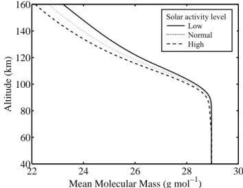
Fig. 2. Mean molecular mass a function of altitude.
Assuming that the mass density profile is proportional to the number density profile, i.e. composition is constant with al-titude, allows the atmospheric mass density to be related to the Rayleigh lidar signal as follows:
ρ (z) ∝ N (z) z2 (4)
Equation (4) shows that the signal measured by a Rayleigh lidar is proportional to the atmospheric mass density, so long as the above assumptions are valid, i.e. the composition of the atmosphere does not change.
The changing composition of the atmosphere above
∼95 km causes the Rayleigh backscatter-cross-section (Eq. 3) of “air” to change with altitude (Fig. 1) so that Eq. (2) is no longer valid. Composition changes also affect the mean-molecular-mass (Fig. 2) so that the number-density profile is no longer proportional to the mass-density profile above 95 km and so Eq. (4) is also no longer valid. These two effects are inherent in the signal recorded by all Rayleigh li-dars and cannot be separated or removed; therefore these ef-fects have been combined for the purpose of this study and are jointly referred to as signal effects.
3 Temperature determination algorithm
In order to determine an atmospheric temperature profile, a Rayleigh lidar measured photon-count profile is first cor-rected for range (Eq. 4) and is then scaled to an atmospheric model so that it represents a relative mass-density profile,
ρrel, i.e. the model is used to estimate the proportionally
con-stant applicable to Eq. (4). At this point the relative mass density profile is reasonably well scaled to the actual atmo-spheric mass density profile.
A relative pressure profile can be determined by integrat-ing the mass-density profile usintegrat-ing the hydrostatic equation by
the repeated application of Eq. (5). This integration proceeds from the top of the density profile downward;
Prel(z − 1z) = Prel(z) + ρrel(z − 1z, z)g(z)1z (5)
where ρrel(z−1z, z) is the average mass density for the alti-tude range from z−1z to z.
To initiate, or seed, this integration the pressure (or tem-perature) at the top of the mass-density profile is required; typically this is taken from a model atmosphere. Seeding the integration in this way may cause an offset in the pres-sures at the top of the calculated relative pressure profile; the magnitude of this offset is proportional to the differ-ence between the actual atmospheric pressure, which is un-known, and the model pressure used. As the integration proceeds downward in altitude by the repeated application of Eq. (5) density increases and the second term in Eq. (5), [ρrel(z−1z, z)g(z)1z], becomes larger so that the error
in-troduced by the choice of seeding pressure on the calculated relative pressure profile diminishes.
The relative pressure profile calculated using Eq. (5) will have the same scaling factor to the actual pressure profile as the relative mass density profile has to the actual atmospheric mass density profile as shown in Eq. (6).
Prel
Patmos
= ρrel ρatmos
=K (6)
By applying the ideal gas law to the relative mass-density and pressure profiles; the temperature profile, T , can be de-termined; T = Prel Rρrel = KPatmos RKρatmos = Patmos Rρatmos (7) Equation (7) shows that temperatures calculated in this way are absolute even though both the mass-density and pressure profiles are relative.
The gas constant, R, used in Eq. (7), is a function of the mean molecular mass of the gas and so changes with alti-tude. Thus, the processing of Rayleigh lidar measurements to obtain temperature profiles is dependent on the composi-tion of the atmosphere. This effect will be referred to as the processing effect.
4 Rayleigh backscatter cross sections
The simulations used in this study model the backscatter from nitrogen and oxygen molecules as well as argon and oxygen atoms. Other species exist in such small concentra-tions that their effect on the lidar signal and retrieved tem-peratures is insignificant. The Rayleigh backscatter cross-sections for the included species are determined using the same procedure as described by Stergis (1966) which re-quires the refractive index and depolarization factor for each species. Updated refractive index values for O2and N2were
obtained from Washburn (http://www.knovel.com/knovel2/
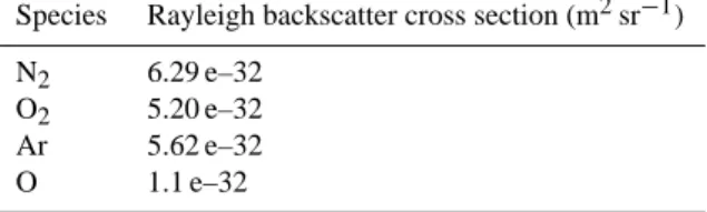
Table 1. Rayleigh backscatter cross-sections at 532 nm.
Species Rayleigh backscatter cross section (m2sr−1)
N2 6.29 e–32
O2 5.20 e–32
Ar 5.62 e–32
O 1.1 e–32
Toc.jsp?BookID=735). The refractive index for argon was taken from Bodhaine (1979) and the Rayleigh backscatter cross-section for O was determined from the values given by Stergis and assuming a λ−4wavelength dependence.
The values of the Rayleigh backscatter cross-sections used in this study are given in Table 1.
5 Method
The NRLMSISE-00 (Naval Research Laboratory Mass Spec-trometer, Incoherent Scatter Radar Extended Model) (Pi-cone et al., 2002) model was used to simulate Rayleigh li-dar photon-count profiles based on the composition of the at-mosphere as well as the Rayleigh backscatter cross-sections and the molecular masses of the four most abundant molec-ular species. The simulated photon-count profiles therefore include the effects of the changing composition of the atmo-sphere with altitude.
The simulated photon-count profiles are idealised in that they contain no photon counting (Poisson) noise or back-ground, due to scattered moon light etc., as are inherent in all measured lidar photon-count profiles. In addition the simu-lated profiles are stored as real numbers rather than integers in order to maintain the precision of the simulation. Simu-lated profiles generated under these conditions can be con-sidered ideal in that they do not contain any of these effects that normally degrade real measurements thus allowing the study to be performed without the influences of these effects. The MSIS model accepts several input parameters: day of year, time of day, latitude, longitude, F10.7 solar flux in-dex, 3 month average of the F10.7 solar flux inin-dex, and ge-omagnetic AP index, which are all used to define the state of the atmospheric model. These inputs allow a large num-ber of combinations of parameters for which lidar photon-count profiles can be simulated, a few representative exam-ples were selected and are presented here. All of the simula-tions presented here use MSIS inputs representing 00:00 UT on 1 January at a longitude of 0 deg. Simulations were per-formed for a set of three solar activity parameters (Low, Nor-mal and High) and for three latitudes (Low, Mid and High); the corresponding MSIS inputs are defined in Table 2. Sim-ulation for other times of year have also been performed, the results of these simulations are similar to those presented for
22 P. S. Argall: Upper altitude limit for Rayleigh lidar
Table 2. MSIS input parameters used for simulating atmospheric
composition.
Activity level Low Normal High
3 month average of the F10.7 solar flux 75 150 275
F10.7 solar flux, daily 75 150 275
AP index, daily 5 12 50
Low latitude Mid latitude High latitude
10 35 75 90 100 110 120 130 140 80 90 100 110 120 130 140
Integration Start Altitude (km)
Altitude (km) 0.1 0.1 1 1 1 2 2 2 4 4 6 6 8 10
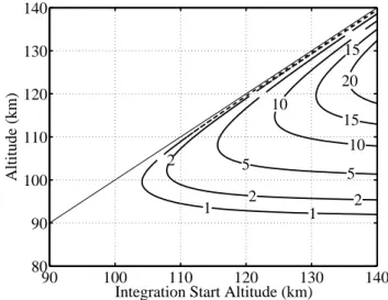
Fig. 3. Contours of temperature bias (K) caused by using the
stan-dard Rayleigh lidar retrieval technique applied to measurements simulated using atmospheric composition taken from the MSIS model for mid-latitude, normal solar activity conditions. See Sect. 5 for further details.
1 January except that the magnitude of the biases are typi-cally smaller, by up to 50% at other times of the year.
A Rayleigh lidar signal was calculated based on the MSIS number densities and the Rayleigh backscatter cross-sections (Table 1). Temperature profiles were calculated from the simulated signal using:
1. the standard Rayleigh retrieval method (no correction), 2. standard Rayleigh analysis with an applied correction
for the effects of composition changes on the measured signal (signal correction),
3. standard Rayleigh analysis with an applied correction for the effects of composition changes on the data pro-cessing (propro-cessing correction), and
4. standard processing with both of the above corrections applied. 90 100 110 120 130 140 80 90 100 110 120 130 140
Integration Start Altitude (km)
Altitude (km) 1 1 2 2 2 5 5 10 10 15 15 20
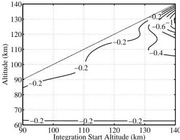
Fig. 4. Similar to Fig. 3 except that the signal correction has been
applied to the simulated photon-count profiles.
The temperature profile calculated when both corrections are applied is taken as the standard to which the other uncor-rected temperature profiles are compared.
Figure 3 shows the temperature bias for simulations at mid-latitude under normal solar activity conditions when no correction for composition changes is applied (no signal cor-rection and no processing corcor-rection). The abscissa indicates the altitude of the top of the temperature retrieval while the ordinate corresponds to the altitude range of the temperature retrieval. The upper left section of the figure is blank as the temperature is not determined at altitudes above the top of the retrieval. Figure 3 shows that for a Rayleigh lidar able to measure useful backscatter from as high as 110 km, once 10 km has been removed from the top of the profile to re-duce the seeding errors; the error at 100 km due to compo-sition changes is of the order of 0.1 K. For a lidar 20 times more powerful than this, which can measure backscatter up to 120 km, the temperature bias due to composition changes is about 2.5 K at 110 km.
It is common to remove 1.5 scale heights from the top of the temperature profile to reduce effects of the seed tempera-ture to an acceptable level. For a temperatempera-ture profile starting at 110 km this corresponds to removing about the top 10 km. The altitude range to be removed increases with altitude in the lower thermosphere.
Temperature biases for the case where the lidar signal is corrected but no processing correction is applied are shown in Fig. 4. A comparison of Fig. 3 and Fig. 4 shows that the result of applying a signal correction without applying a processing correction increases the temperature bias sig-nificantly.
The bias in the temperatures profiles determined without a signal correction but with the application of a processing correction is shown in Fig. 5; again the magnitude of the bias
90 100 110 120 130 140 80 90 100 110 120 130 140
Integration Start Altitude (km)
Altitude (km) −1 −1 −1 −2 −2 −2 −4 −4 −6 −6 −8 −8 −10 −12
Fig. 5. Similar to Fig. 3 except that the processing correction has
been applied.
is greater than applying no correction at all. In this case the calculated temperatures are too low. It is apparent that mak-ing no correction for composition changes leads to a smaller bias in the calculated temperature profile than providing a correction for either the signal or the processing alone.
If detailed composition measurements were available along with Rayleigh lidar measurements it would be possible to accurately correct the calculated temperature profiles for composition changes. However composition measurements at these altitudes are currently not routinely available. Cur-rently the best ongoing source of information on composi-tion is a model atmosphere such as MSIS. Using atmospheric composition data from MSIS as the basis for providing cor-rections for Rayleigh temperature profiles will lead to some bias in the derived temperatures due to differences between the model and actual composition. In order to provide an assessment of the magnitude of this bias it is useful to deter-mine the bias in cases where a single “standard” composition is used to provide corrections for measurements taken with a variety of composition scenarios. Figures 6 and 7 show the temperature bias due to using composition corrections (both for signal and processing) based on moderate solar ac-tivity for Rayleigh lidar photon-count profiles simulated for quite and disturbed solar conditions respectively. For the re-sults presented in these two figures, the temperature retrieval algorithm is seeded with a temperature appropriate for the photon-count profile simulation conditions, i.e. the tempera-ture for the quite and disturbed conditions respectively. The temperature biases shown in Figs. 6 and 7 are significantly smaller than those shown in Fig. 3 demonstrating that for the range of atmospheric composition changes between low and high solar activity the bias caused by applying a “standard correction” for composition is significantly less than the bias in the case where no correction is applied.
90 100 110 120 130 140 60 70 80 90 100 110 120 130 140
Integration Start Altitude (km)
Altitude (km) −1 −0.6 −0.4 −0.2 −0.2 −0.2 −0.2 −0.2 −0.2 −0.2
Fig. 6. Mid latitude – measurements made during quiet solar
activ-ity and processed assuming moderate solar activactiv-ity, except that the temperatures used to seed the retrieval are for quite solar activity.
90 100 110 120 130 140 60 70 80 90 100 110 120 130 140
Integration Start Altitude (km)
Altitude (km) 0 0.2 0.2 0.2 0.4 0.4 0.4 0.4 0.4 0.4 0.4 0.4 0.4
Fig. 7. Mid latitude – measurements made during disturbed solar
activity and processed assuming moderate solar activity, except that the temperatures used to seed the retrieval are for disturbed solar activity.
Figure 6 shows that for photon-count profiles starting at 140 km and measured under quite solar conditions and pro-cessed with corrections based on moderate solar activity, using the seed temperature for quiet solar conditions, the maximum temperature bias is about 2 K at 130 km reducing to 0.8 K at 120 km. Figure 7 shows that for photon count profiles measured under disturbed solar conditions and pro-cessed as for Fig. 6 the temperature bias is less than 1 K at all altitudes. These results show that the changing composition of the atmosphere above the mesopause does, as expected, have an effect on Rayleigh lidar temperature measurements; however applying corrections based on a composition profile
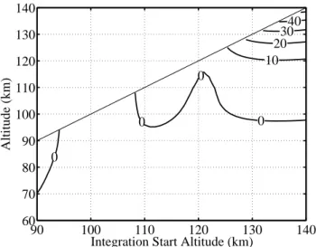
24 P. S. Argall: Upper altitude limit for Rayleigh lidar 90 100 110 120 130 140 60 70 80 90 100 110 120 130 140
Integration Start Altitude (km)
Altitude (km) 0 0 0 0 10 20 3040
Fig. 8. Mid latitude – measurements made during quiet solar
ac-tivity and processed assuming moderate solar acac-tivity, including the selection of the seeding temperature.
derived from a model is sufficient to reduce the bias to quite low levels even for measurements extending to an altitude of 140 km. It should also be noted that the bias could likely be reduced further by providing corrections based on MSIS data for the appropriate solar activity, although it becomes diffi-cult to assess the residual errors as the differences between the MSIS composition data and the actual composition is not well known.
More significant bias at the top of Rayleigh lidar temper-ature profiles are caused by the error in the pressure or tem-perature used to seed the retrieval algorithm. For the current generation of high power Rayleigh lidars it is possible to use co-located sodium lidar temperature measurements to seed the Rayleigh temperature retrieval algorithm, so long as the top of the Rayleigh measurements is in the altitude range of the sodium lidar, 85 to 105 km (Dao et al., 1995; Alpers et al., 2004). Figure 8 shows biases for the same conditions as used for the simulation results shown in Fig. 6, except that the seed temperature is taken for moderate solar activity. In this case the Rayleigh lidar temperatures are too hot by up as much as 30 K when the retrieval is initiated at 140 km and the top 10 km is removed. The contours in the upper right of the figure are almost horizontal; this shows that extending the altitude of the integration initiation does not improve the accuracy of the retrieved temperature at a given altitude, i.e. the Rayleigh lidar temperature at 120 km is 10 K too hot if the retrieval is started at 130 km or at 140 km.
The temperature biases shown in Fig. 9 are due to mea-suring Rayleigh lidar photon-count profiles under disturbed solar activity conditions and processing them assuming mod-erate solar activity. The retrieved temperatures are more than 40 K too cold at 130 km when the integration is started at 140 km. As with Fig. 8 the contours in the upper right of the
90 100 110 120 130 140 60 80 100 120 140 70 90 110 130
Integration Start Altitude (km)
Altitude (km) −60 −40 −20 −10 −10 −2 −2 −2 0 0 0 0 2
Fig. 9. Mid latitude – measurements made during disturbed solar
activity and processed assuming moderate solar activity, including the selection of the seeding temperature.
figure are approximately horizontal showing that increasing the integration start altitude does not reduce the temperature error at lower altitudes.
6 Conclusions
The standard Rayleigh lidar technique is relatively insen-sitive (bias typically <0.1 K) to atmospheric composition changes with altitude so long as the temperature retrieval al-gorithm is started at or below 110 km and the top 10 km of the temperature profile is removed.
For measured photon-count profiles extending above 110 km, modifications to the standard Rayleigh data analy-sis algorithms, employing model (NRLMSISE-00) composi-tion informacomposi-tion, provide usefully accurate correccomposi-tions (typi-cal bias <1 K), even without specific knowledge of solar ac-tivity parameters.
The limiting factor in extending Rayleigh lidar tempera-ture measurements is the temperatempera-ture (or pressure) used to seed the retrieval algorithm. Unless there are independent, coincident, accurate temperature measurements available at the integration start altitude the errors introduced by the seed-ing temperature uncertainty are likely to be much greater than those due to the uncertainty in atmospheric composi-tion.
Acknowledgements. Canada’s National Science and Engineering
Council (NSERC) is thanked for funding this work.
Topical Editor F. D’Andrea thanks two referees for their help in evaluating this paper.
References
Alpers, M., Eixmann, R., Fricke-Begemann, C., Gerding, M., and Hoffner, J.: Temperature lidar measurements from 1 to 103 km altitude using resonance, Rayleigh, and Rotational Raman scat-tering, Atmos. Chem. Phys, 4, 793–800, 2004.
Bodhaine, B. A.: Measurement of the Rayleigh scattering properties of some gases with a nephelometer, Appl. Opt., 18, 121–125, 1979.
Chanin, M. L.: Review of Lidar contributions to the description and understanding of the middle atmosphere, J. Atmos. Terr. Phys., 46, 987–993, 1984.
Dao, P. D., Farley, R., Tao, X., and Gardner, C. S.: Lidar observa-tions of the temperature profile between 25 and 103 k: evidence of strong tidal perturbation, Geophys. Res. Lett., 22, 2825–2828, 1995.
Gardner C. S., Senft, D. C., Beatty, T. J., Bills, R. E., and Hostetler, C. A.: Rayleigh and Sodium Lidar techniques for measuring middle atmosphere density, temperature and wind perturbations and their spectra, World Ionosphere/Thermosphere Study Hand-book, edited by: Liu, C. H., 2, 148–187, 1989.
Hauchecorne, A. and Chanin, M. L.: Density and Temperature ob-tained by lidar between 35 and 70 km, Geophys. Res. Lett., 7, 565–568, 1980.
Kent, G. S. and Wright, W. H.: A review of laser radar measure-ments of atmospheric properties, J. Atmos. Terr. Phys., 32, 917– 943, 1970.
Picone, J. M., Hedin, A. E., Drob, D. P., and Aikin, A. C.: NRLMSISE-00 empirical model of the atmosphere: Statistical comparisons and scientific issues, J. Geophys. Res., 107, 1468, doi:10.1029/2002JA009430, 2002.
Shibata, T., Kobuchi, M., and Maeda, M.: Measurements of density and temperature profiles in the middle atmosphere with a XeF lidar, Appl. Opt., 25, 685–688, 1986.
Sica, R. J., Sargoytchev, S., Argall, P. S., Borra, E. F., Girard, L., Sparrow, C. T., and Flatt, S.: LIDAR Measurements taken with a large-aperture liquid mirror. 1. Rayleigh scatter system, Appl. Opt, 34, 6925–6936, 1995.
Stergis, C. G.: Rayleigh scattering in the upper atmosphere, J. At-mos. Sci., 28, 273–284, 1966.