THE ECONOMICS OF THE NATURAL GAS SHORTAGE (1960-1980) Paul W. MlacAvoy Robert S. Pindyck Report # MIT-EL 74-011 September, 1974
SHORTAGE (1960-1980)
by
Paul W. MacAvoy and Robert S. Pindyck Massachusetts Institute of Technology
Energy Laboratory Report o. MIT-EL 74-011
TABLE OF CONTENTS
PREFACE
CHAPTER 1 -- Government Regulation and Industry Performance, 1960-1974 1.0 Introduction
1.1 Production and Distribution of Natural Gas
1.2 Gas Field Price Regulation by the Federal Power Commission
1.3 The Behavior of Field and Wholesale Markets Under Price Controls 1.4 Summary
CHAPTER 2 -- Alternative Regulatory Policies and the Natural Gas Shortage, 1974-1980
2.1 Strengthened Regulation
2.2 Elimination of Regulation of Field Prices
2.3 Assessing the Effects of These Policy Alternatives
2.4 The Effects of Gas Policy Changes on Producers, Consumners, and Others
2.5 The Rationale for the Shortage and Regulation
CHAPTER 3 -- The Structure of the Econometric Model of Natural Gas 3.1 Overview of the Econometric Model
3.2 Structural Equations for Gas and Oil Reserves 3.3 Structural Equations for Production of Gas
3.4 Equations for Reserves and Production of Offshore Gas 3.5 Pipeline Price Markup Equations
3.6 Structural Equations for Wholesale Demand for Natural Gas and Fuel Oil
3.7 Connecting Supply Regions with Demand Regions 3.8 Summary of the Structural Model
Appendix: Wholesale Demand for Gas by a Regulated Utility CHAPTER 4 -- Statistical Estimation of the Econometric Model
4.1 Estimation Methods 4.2 The Gas-Oil Data Base
4.3 Estimated Equations for Gas and Oil Reserves 4.4 Estimated Equations for Production of Gas
4.5 Estimated Equations for Offshore Reserves and Production 4.6 Estimated Equations for Pipeline Price Markup
4.7 Estimated Equations for Wholesale Demand for Natural Gas 4.8 Estimated Equations for Wholesale Oil Demand
4.9 Interregional Flows of Gas in the Econometric Model 4.10 Summary
CHAPTER 5 -- SIMULATIONS OF THE ECONOMETRIC MODEL 5.1 Historical Simulations
5.2 Use of the Model for Forecasting and Policy Analysis 5.3 The Demand Function for Liquified Natural Gas
PREFACE
An appraisal of the natural gas shortage requires both a detailed description of political and technical institutions, and an economic analysis of the evolving performance of this industry. Not much can be said without a description of the legal controls on producing gas in the South for delivery to consumers in the North, or without an economic ana-lysis of price and quantity relationships on both the production and demand sides of gas markets. There also has to be some indication of the present size of the shortage, of the means by which the industry would respond to policies to reduce the shortage, and how much time this response would take.
The approach here divides the institutional and analytical materials into two parts. First, the political and institutional frame of reference is described and the present-day natural gas shortage is estimated in Chapter 1; and forecasts are made of the effects on this shortage of various alternative regulatory policies in Chapter 2. Second, a large-scale econometric policy model of natural gas markets- both field markets and wholesale distribution markets---is presented in Chapters 3,4 and 5 in some detail. Thus the model is described in Chapters 3-5 after it is used for evaluating alternative policies in Chapter 2. This is done so that non-econometricians can deal, with least obfuscation and delay, with the results from the policy analyses, leaving it to the more technically oriented analyst to check these results against the model and simulation descriptions in Chapters 3-5. However, frequent references are provided in Chapter 2 to the technical description in subsequent chapters, so that documentation or analysis can be obtained where needed even by the non-econometrician.
ii
The plan of the book, then, is as follows:(l) introduction to the natural gas shortage and the technical-regulatory frames of reference for explaining the present extent of the shortage. This is followed by (2) an analysis of alternative policies for dealing with the shortage, using the econometric policy model described in technical detail in Chapters 3, 4, and 5. For those seeking to understand the general nature of the present policy problems in the natural gas industry, Chapters 1 and 2 should suffice; for those interested in the development of an econometric model designed specifically to assess the efficiency of alternative regula-tory policies in dealing with shortages, Chapter 3, 4, and 5 should be of particular interest.
Acknowledgements
This study reports on the results of a National Science Foundation project to develop an econometric policy model of natural gas, under grant no. GI-34936. The first phase of the project was described in Sloan School of Management working paper no. 635-72 (December, 1972), and the second phase was reported in "Alternative Regulatory Policies for Dealing with the Natural Gas shortage" by P.W. MacAvoy and R.S. Pindyck in the Bell Journal of Economics and Management Science, vol. 4, no. 2, Autumn, 1973. A project of the scope of the gas policy model has to be undertaken as a group effort. We received the substantive support and assistance of a number of colleagues here at M.I.T., and without this extended help this project would not have been completed. The assistance of Krishna Challa, doctoral candidate in the Sloan School, was extensive in the construction of the model of reserves; as noted in Chapter 3, the
formulation of structural equations for reserves is essentially that in Krishna Challa's doctoral dissertation entitled "Investment and Returns
in Exploration and the Impact on the Supply of Oil and Natural Gas Reserves". Similarly, Ira Gershkoff and Philip Sussman played substantial roles in the formulation of parts of the model--Gershkoff in the price markup equations and input-output table, Sussman in the model for offshore reserves and production. Sussman's work, now part of the model, is described in "Supply and Production of Offshore Gas Under Alternative Leasing Policies", an M.S. dissertation at the Sloan School of M.I.T. (1974). Robert Brooks and Marti
Subrahmanyam, M.I.T. doctoral students, played major roles in the construc-tion of natural gas demand equaconstruc-tions, and Bruce Stangle, also a doctoral student, helped us in the development of the oil demand equations. Birgul Erengil, an M.S. student at Sloan, provided assistance in the documentation of our final results. Finally, Kevin Lloyd, also an M.S. student, took on
the task of managing all of the computer operations involved in constructing the model, prepared and conducted most of the simulation exercises, and assisted in the estimation of most parts of the model. We are indebted to those cooperative and productive colleagues.
The computational work was performed at the Computer Research Center
of the National Bureau of Economic Research in Cambridge, Massachusetts, and relied on the TROLL system for the estimation and simulation of the model. Also,
the data base was constructed and maintained at the NBER Computer Research Center. The considerable assistance that we received in the use of TROLL
from Mark Eisner and Walt Maling of the NBER, as well as others on the staff of the Computer Research Center, was invaluable in the construction of the model, and is extremely appreciated.
iv This project has been one of many undertaken at the M.I.T. Energy Laboratory. We wish to express our appreciation to our colleagues in the Energy Laboratory, particularly Morris A. Adelman, Gordon Kaufman, Jerry Hausman, Paul Joskow and Martin Baughman for comments on earlier drafts and help in reformulation of the model in the final phase. Sub-stantial assistance was provided by Edward Erickson, Dale Jorgenson, Edward A. Hudson, Daniel Khazzoom, Edward Kitch, Robert Spann, and Lester Taylor as a result of their reviews of the preliminary draft of this manu-script. Finally, a large number of readers of the earlier version of the model--as well as users of the model--provided comments and criticisms that added to our efforts in reformulating the econometric analysis.
This legion of critics, mercifully granted anonymity, made the work towards the final version worthwhile.
Cambridge, Massachusetts September, 1974
GOVERNMENT REGULATION AND INDUSTRY PERFORMANCE, 1960 - 1974
1.0 Introduction
The natural gas industry in the United States has experienced sub-stantial shortages in the last few years. Rather than hour-long queues, as at gasoline stations in early 1974, the natural gas shortage of the 1970's has resulted in partial or total- elimination of service for groups of consumers, both residential and industrial, that demand gas rather than other fuels. Service has been terminated for interruptible buyers--those taking gas only part--time or off-peak--and new potential full-time consumers have not been allowed to connect to delivery systems. At many locations, industrial and commercial consumers have been told to replace gas with oil at least on a part-time basis. The sum total of these
unfilled demands has been fairly extensive. The Federal Power Commission found that interstate gas distributors were 3.7 percent short of meeting consumption demands of communities and industries in 1971 and that they are expected to be 10 percent short of demands in 1974.1
There appears to be small prospect for amelioration of shortage
conditions in the near future, Unless there are unexpected discoveries, or unless FPC regulation changes significantly, excess demand is expected to grow to more than one-quarter of total demands This is not only the prediction of econometric forecasts. Indeed. the FPC staff of gas experts
cf. National Gas Supply and Demand, 1971-1990 (FPC Bureau of Natural as, Washington D.C., February, 1972).
This forecast is the result of use of an econometric policy model to stmu--late continuation of present geological and regulatory constraints over tihe period 1975-1980. The model is described in Chapters 3-5, and the simulations outlined in Chapter 2, below.
-2-forecasts that, assuming continuation of present day regulatory conditions, the shortage will grow to be as large as 20 percent of demands by 1980.3 Those that are now being told to curtail consumption or toswitch to other
fuels are not likely to be told anything different unless public policies change.
Consumers in some regions of the country have fared worse than those in other regions in obtaining the gas they demand. So far, buyers in the North Central, the Northeast and the West--in that order--have incurred most of the shortage. New residential buyers and new as well as some old industrial buyers in those regions continue to be kept off distribution
systems. By the late 1970's, shortages in the North Central region could exceed one-half of demands. If this occurs, then industrial and commercial establishments will face 100 percent elimination of supply, in order that there would still be enough gas to meet the "old household" consumption draughts on local utilities. In other regions, industry may not be cut off entirely, but substantial industrial buyers seeking to expand their uses of gas would face curtailment at most locations. Some of these buyers should be able to obtain more supply in the South, outside of regulation and the shortage by relocating their activities 4 If they were to relocate in significant numbers, there would be important changes in regional industrial development. Industrial growth in the energy-related industries of the upper Midwest would be reduced relative to the rest of the country.
cf. National Gas Supply and Demand, op, cit.; this forecast calls for almost as much shortage as the gas econometric forecast; presumably it is based on continuation of present price regulation (although this is not explicit).
4
These statements are once again predictions from the econometric model described in detail in Chapters 3-5. The forecasts for 1975-1980 shortage
These conditions should elicit questions from many consumers in the next few years. As service is curtailed, they might well ask, where the shortage came from. In particular, they should know how long it will last under continuation of present conditions in gas markets. and if the shortage can be reduced at an earlier date by policy changes of companies and governments.
It is important to know first where the shortage came from," so that policies specific to type of consumer, location and time period can be formulated to eliminate the shortage-creating conditions. The next section of this chapter (1.1) specifies the details of the production process in gas fields necessary for an understanding of the shortage sit-uation. In Section 1.2, there is a lengthy description of gas field price regulation by the Federal Power Commission. Regulation has become an important precondition of production, and certain aspects of regulation can be seen to have caused the development of the shortage. The third section below (1.3) describes the behavior of field markets under present regulatory controls as compared to "no control" conditions. The conclu-sions here, showing the effects of controls, give credit to the regulators for the shortage, Subsequently, Chapter 2 attempts to answer the question,
"how long will there be an extensive shortage" under present conditions. Also, stud-es ae presented. of the effects from alternative governmental policies that show that extensive change in the present method of control, and present
price levels, can have substantial ameliorative effects on the shortage. 1.1 Production and Distribution of Natural Gas
The field markets for natural gas center around transactions In which petroleum companies dedicate newly-discovered reserves of natural gas for production into pipeline transmission lines. Major petroleum
5
The forecasts are based on simulations with the econometric policy model described in Chapters 3-5,
-4-companies, along with smaller independents, initiate activities by using seismic logging and the drilling of wells to "discover" new gas reserves, or to complete the "extension" or the "revision" of previously known
reserves. They bring gas production to the surface where liquid by-products are removed. Then the pipeline companies take the gas in the field and deliver it to wholesale industrial users or to retail distributing com-panies, that in turn deliver it into individual households, commercial establishments or to retail industrial users. Ultimately, more than 45 percent of the natural gas production goes to residential and com-mercial consumers, while the rest is consumed as boiler fuel or process material in industry.
Reserves, production, and the pattern of consumption depend on certain technical and economic conditions. The most important of these relationships, in terms of an "economic model," are sketched in the
flow diagram below. Each of the boxes will be dealt with later in detail (since this is a simplified version of the flow diagram for the econo-metric model described in Chapters 3-5); but it is posited here that prices of oil and gas are critical policy variables, such as the leasing practices on government lands that determine production. Also, oil and gas prices are policy-related determinants (along with non-policy variables such as other fuel prices and consumer incomes) of residential or industrial
6
The percentage of total consumption by residential and commercial buyers was 45 percent in 1962, and 43 percent in 1968: as the natural gas shortage appeared on the horizon, the amount of residential consumption declined. cf. Federal Power Commission, Statistics of Natural Gas Pipelines (annual); cf. also S. Breyer and PW. MacAvoy, "The Natural Gas Shortage and Reg-ulation of Natural Gas Producers," Harvard Law Review (vol. 86, no. 6, April 1973), pp. 977 et seq.).
demands for gas.7 1.1.1 Field Markets8
The gas reserves committed by the producing companie8 to ) lI)lfille A P 1tl'l mtj4 I II 1tl1l .11 ltll11 tIl1tll. l 1 1 t F* 1 | 1td I IIP Itltllq ll ll llp I ito q. q '1q1- I. ll
panies ascertain that there are inground deposits of (1) "assoc.ated" gas in newly discovered oil reservoirs and (2) "nonassociated" gas found in reservoirs not containing oil.
Figure 1.1 Simplified Diagram of the Econometric Model
Field Markets Wholesale Markets
crude oil gas field prices - prices
wells drilled
[ gas reserve discoveries -I gas reserve extensions
} gas reserve revisions
-. 1
J
total additionsI
to gas reserves l tota reserves gas production outof reserves -~1 -A industrial and _other demands I total demands for annual gas production
F-gas shortage
7
These are all statements of empirical relations, based on the equation relationships formulated in Chapter 3 and fitted in Chapter 4 below.
8
This subsection, like the previous one, describes in straightforward terms the equation relationships in the econometric model of Chapters 3 to 5
below. The description is based on the direction of cause-effect relationships found below, and seeks to indicate extent by including coverage of only the
important relationships with policy or with certain non-policy variables. other prices, fnal product outp
L___
pipeline pri at wholesale a residential and commercial demandsfor gas at wholesale
I
I
p w I _ . . --- -- -1--
~~~~~~~~~~~~~~~~~~~
I . . _I m _ _._ +mmr" __ - 46 a2
a -E I IIF
I.
-6-Companies claim such reserves as a result of new discoveries, or extensions or revisions of previous discoveries (where extensions result from stepping out beyond the limits of known field boundaries, and revisions are changes in estimates of reserves in place within known field boundaries).
After reserves are known to exist, the producers "dedicate" them in a con-tract calling for production over a five-to-twenty year period. In effect, the producers estimate the size of newly-found inground deposits and provide sufficient documentation to support contract commitments to pipelines for production over that period. Of course, reserves are never known for certain (as indicated by extensions and revisions each year), so that the contracts are in effect "futures" agreements or promises to deliver an uncertain volume of a commodity.
The process of adding to reserves begins long before commitments to pipelines. Years earlier, the producer undertakes geophysical exploratory work to show the existence of a potential inground hydrocarbon reservoir,
after which he sinks wells into the reservoir to determine whether there is oil, gas, water, or whatever. The decision to conduct preliminary geophysical research and drill wells is essentially an investment decision under uncertainty; as the potential profitability of the investment increases, the number of wells drilled increases and total discoveries increase.
Profitability depends upon future prices and costs, which relate in a com-plicated but positive way to present prices and costs. Thus if present prices increase, there should be an increase in exploratory work; this
9In the econometric model, tis process is described as being divided between decisions on "well-drilling" and "size of discovery" per success-ful well. Operating at the intensive margin implies increased drilling and reduced size of find per successful well. Operating at the extensive margin-implies increased drilling and an increase in the size per success-ful well. Both together imply rising supply of reserves as prices increase.
would lead, in a year or two, to additional drilling activity and subse-quently to the offering of additional reserves for sale to pipeline
buyers. Of course prices are not the only determinant of reserves. There is a fixed stock of gas to be discovered in a region, and it is suspected that the larger and most profitable volumes are discovered and dedicated there first. Technical progress in drilling or production techniques could compensate for the limits in any area by pushing down costs of finding the smaller volumes; also, some areas may not yet have experienced the initial
10
stages. But over time, at fixed prices and costs, we should observe that the volume of discoveries declines per well drilled.1
The discovery of reserves is the first step in the production process. The second step is contractual dedication to the production of gas and its
1 0
This again is dealt with explictly in the econometric model described in Chapters 3-5. The summary here does not take account of the relative importance of the variables (a) prices (b) technical progress (c) earlier discoveries in explaining additions to reserves. The equations in Chapter 4 provide this important detail.
1 1At the present time, the limits on total reserves do appear to be
con-straining. We are not "out" of discoverable reserves in the United States. The sum total of past production and of present discovered reserves, as of 1970, totaled 648 trillion cubic feet, less than 40 percent of the amount of ultimate discoverable reserves expected in most forecasts. The amount remaining to be discovered has been estimated as 851 trillion cubic feet (by the National Petroleum Council and by the Colorado School of Mines' Potential Gas Committee), and as 2,100 trillion cubic feet (by the U.S. Geological Survey). (National Petroleum Council, U.S. Energy Outlook: Oil and Gas Availability, U.S. pept. of the Interior, Tables 291 and 292 on page 367; Potential Gas Agency, Minerals Resources Institute, Colorado School of Mines, Potential Supply of Natural Gas in the United States, October 1971 (the latest report, issued in December 1973, gives 1,146 trillion cubic feet; U.S. Geological Survey, Circular 650, "U.S. Mineral Resources," states that the range of estimates is between 1,178 and 6,600 trillion cubic feet.) Of course the amount actually found and put in the reserves category will depend on the level of exploratory activity, on costs of development, and on the prices offered by the pipeline buyers. These are the most important (technical and economic) limiting factors; the reserve estimates show enough additional reserve inventory to support at least two decades of production (at forecast rates exceeding 30 trilli-on cubic feet per annum).
-8-movement in the pipelines to final consumers. The amount of production depends on a number of geological, engineering, and economic factors. Production cannot take place at rates greater than some fixed percent of reserves per annum, because of technical limits (sandstone in the reservoirs is not completely permeable so that the gas cannot move to the well faster) and because of economic costs (faster rates of depletion may reduce the economic value of any remaining reserves by "channeling" and sealing off parts of the reservoir from further production). But up to these limits, more production can take place at higher short-run costs. Thus, with a given reserve inventory, if prices are high enough to compensate for higher costs of further drilling investment, the production rate can be increased.
Field markets for natural gas are, thus, similar to minerals or raw materials futures markets in which present deposits are dedicated for future production and refining. The important characteristics of these markets generally are that more reserves will be dedicated if the buyers offer
higher prices, and that the lag adjustment process bringing forth additional reserves by higher prices is likely to be long. Also, production out of dedicated reserves is limited by technical or economic factors, but is
likely to be greater, the larger the volume of reserves available and the higher the contract prices.
1.1.2. Wholesale Markets
The buyers of reserves at the wellhead are for the most part natural gas pipelines providing gas under long--term contract to industrial consumers and retail public utility-companies. The amounts of their annual deliveries
1 2That is, in the econometric model below, technical and economic
condit-ions determine production out of reserves, so that the level of production will be greater, the greater is the volume of reserves in place and the higher are prices in the contract commitment.
determine their demands for reserves to be dedicated at the wellhead. These annual deliveries in turn depend upon the prices they charge for gas at wholesale (paid by industrial consumers and retail-public utilities to the pipelines), the prices for alternative fuels consumed by final buyers, and economy-wide factors such as population, incomes, industrial production, etc., that determine the overall size of energy markets.
Gas wholesale prices, in turn, depend upon field prices and delivery charges for transportation of the gas from the wellhead to the final con-sumer. The pipelines offer instantaneous deliveries of gas as it is burned by the final buyer: they charge a markup over their field pur-chase prices as part of the wholesale price for these services. Markups are determined by the historical average costs of transmission and by the transportation profit margins allowed under Federal Power CommisiHlon reg--lation (at least for the interstate pipelines).
Regulation of the wholesale prices, in fact, builds in significant lags of changes in final prices behind those in field prices. The Federal Power Commission has followed the policy of allowing wholesale prices equal to the markup plus the historical average field price paid for gas at the wellhead. This "rolled in" or average wellhead price changes slowly as a result of higher prices on new field contracts, because new contracts
in any year make up only 5 to 15 percent of all contracts. The full impact of a change in new contract prices is realized only after it has been in effect for almost a decade (assuming O percent of deliveries in each year
come from new contract dedications). This time lag between changes Ln wellhead and wholesale prices softens the impact on consumers of large
increases in new prices in field markets. Also, average transmission costs change very slowly, as new construction costs or allowed returns on capital
-10-change slowly (at least as allowed by the FPC). From 35 to 40 percent of the gas remains in the South Central region of the country where it is produced; approximately 19 percent moves to the Northeast, 20 percent to the North Central, and 7 percent to the western parts of the country. This was the case over much of the 1960's, with only the North Central region showing some increases over the period 1962-1968 (by three tage points, while the North Central region was reduced by the same percen-tage).
The flow diagram shows how all these transactions work out in "normal" circumstances. At a given level of field prices, the additions to reserves meet the needs of the pipelines (as evidenced by their new contract demands).
If not, and there is excess demand, then the prices these pipelines offer in new contracts increase above the previous level. Immediately, this brings forth more production from old contract reserves, brings forth some new
contract reserves, and also cuts back on some of the marginal resale at the pipelines. After a time, the higher new prices also bring forth more new reserves and cut back on the long-term contracts sought by final buyers. Eventually at some level of new contract prices the amount of new reserve commitments by the producers is the same as the amount bought and resold by the pipelines.
1.1.3. The Effects of Shortages on Field and Wholesale Markets
Under "normal" conditions, the reserve and production markets operate to allow each pipeline buyer that "reserve backing" he desires, backing that makes secure the continuation of production to meet his commitments to residential and industrial consumers over the lifetime of their burning
13The process of setting markups on field prices is described in detail in Chapters 3 and 4, using a truncated version (in equation form) of FPC regulatory practice.
equipment. In a "shortage", the new discoveries fall short of the reserve amounts demanded by the pipelines in order to provide for the backing he seeks for his wholesale buyers. Under these conditions, the amount of actual field contract commitments are not equal to total "demands," but are-equal only to "supply." At that point, the pipelines either (1) limit their commitments so as to preserve backing for old
consumers or (2) draw down previously purchased reserves at a faster rate. If the second alternative is taken, production demands of final consumers could be satisfied for some period, as a result of the pipelines calling on existing reserves to produce at a higher rate,(thereby eliminating the reserve backing of old consumers). Thus reserve shortages in field markets may not-be perceived by final buyers whose demands are temporarily satisfied by present production (as was the case in the late 1960's)1 4
Production to meet expanding demands from previous reserve ments cannot be had indefinitely. Eventually, reserves from old commit-ments are reduced sufficiently so that the amount remaining limits the amount of production. As the reserve backing becomes smaller, production tends to fall, and a gap is opened between the demands for production and the amounts available. Many years may pass, however, before decline
in additions to reserves is followed by a shortage of production.
Can the process be reversed? As indicated above, if prices were to increase in new contracts by a substantial amount, then more production could be gotten out of the previously committed reserves (because the price
increase can compensate for additional costs from secondary recovery programs). This effect may be rather small, however, given that reserves have already been greatly depleted. But there would be a longer-term effect caused by
This is surmised 'from the simulations with the econometric model, as shown for the 1960's and 1970's in Chapter 5.
-12-price stimulation of the discovery process. Higher -12-prices would add to incentives for exploratory drilling, and the drilling would increase new discoveries, extensions or revisions of reserves. After these additional reserves have been committed, the amount of production would then again
15
be increased. At the same time, over this extended period, demands for production would be curtailed by the higher price. Total demands would have increased because of increases in the size of energy markets
(and increases in the prices of alternative fuels). But high gas prices should slow down the accumulation of new customers, so as to have a dampening effect on the size of the increased gas demands.
The combination of both reserve and demand incentives should be to reduce the excess demands. But it may take several years before the full effects of a price change are felt in field and wholesale markets. The period should be much longer than that required to complete the process of market clearing in grain or metals commodity markets. Under some con-ditions, however--with large price increases and new government policies on reserve discovery--it is expected that most of the shortages expected to occur in each region of the country can be reduced or even eliminated before 1980.
1.2. Gas Field Price Regulation by the Federal Power Commission The history of regulation bearing on the gas shortage began
1954, with the Supreme Court's decision requiring the Federal Power Comr.. missionto regulate the wellhead prices on production into the interstate pipelines. This was an appeal in a case brought by the Attorney General of Wisconsin against Phillips Petroleum Company; Phillips' prices to the pipelines had been increasing, and higher prices were alleged to be contrary
15
As shown by simulation with the econometric model, the results are given in detail in Chapters 2 and 5.
to the best interests of consumers in Wisconsin. In lower court testi-mony and briefs, arguments were made that the gas industry, while regu-lated at the pipeline level by the Federal Power Commission and at the retail level by the state regulatory commissions, was unregulated by government and even worse was controlled by the large field producers at the wellhead. Therefore field price increases, determined by a few large petroleum companies, could be passed through as "costs" in whole-sale prices to result in final price increases to the consumer. Such pass throughs, it was argued, should be curtailed by the introduction of
FPC regulation at the wellhead. The Supreme Court, without explicitly affirming that there was monopoly power in the hands of the producers, found that the Federal Power Commission did have the mandate to regulate
16 the wellhead price.
For the next five years, the Commission attempted to respond to the mandate. Price control at the wellhead covered first those contracts in the Phillips case itself, since that case had been remanded by the court for a finding of "just and reasonable " prices. The FPC first con-trolled price levels in the same way that state public utility commissions set limits on electric power or gas retail prices. The procedure begins by estimating (a) operating costs, (b) the allowed rate of return times the undepreciated original investment, and (c) depreciation of investment per unit of gas produced under a contract. These unit "accounting costs"
Phillips Petroleum Company vs. Wisconsin, 347 U.S. 622 (1954). cf. E.W. Kitch, "Regulation of the Field Market for Natural Gas by the Federal Power Commission," Journal of Law and Economics (XI, Oct. 1968), pp. 243-281; Kitch notes on page 255 that "the court gave no reason for the regu-lation...considering the expertise of the Federal Power Commission... the court gave no indication of how the regulation was to be carried out."
-14-are defined as equal to {[(a) + (b) + (c)]/q} for q annual production. The permissible maximum level for average prices is set equal to these unit costs, or to "costs of service." The "cost finding" approach to price control was not readily applicable to Phillips, because part of the gas was produced with oil, which was not being regulated, and some was produced only after a number of dry wells had been drilled. Attributing previous "dry hole" costs to particular gas contracts, and attributing
joint costs to gas or to oil, resulted in arbitrary limits on prices. Also, the usual standards for finding the proper rate of return--the
aver-age rate of return for public utilities--scarcely applied to an exploration and development company. In fact, higher returns were allowed to compen-sate for exploratory risk, but these were simply stated as being appro-priate. It turned out that the prices proposed by the Commission were higher in some cases than the original prices objected to by the state of Wisconsin.
During this time the Commission, dealing in infinite detail with Phillips, was falling behind. The case had produced more than 10,000 pages of briefs and records; in the meantime, by 1962, more than 2,900
applications for price reviews had been filed by other companies. Man-agement failure--the Commission itself forecast that it would not finish its 1960 caseload until the year 2043 --and the arbitrary nature of regulation together required the FPC to-try other ways of controlling
field prices.l8
The FPC turned to setting the same ceiling price for all transactions within a widely-defined geographical region. Temporary ceilings were set at market levels established a year or two previously (in the fashion of economy-wide "price freezes" common in the later 1960's). This way of regulating resulted in a freeze on prices at the 1958-59 level, so that new gas committed to interstate pipelines after 1961 had to be priced at a level not higher than the 1958-59 level. The freeze was to be temporary and was to be followed by "area rate" decisions which set permanent prices. The permanent prices were to be based on the average historical costs of gas within the region; and, in fact, considerable attention in the area rate proceedings was given over to calculating
regional production costs, investment outlays and rate-of-return averages.
18
James M. Landis was particularly critical of the FPC's performance in the field of natural gas regulation, charging it with delays as well as with disregard of the consumer interest. He wrote:
"The FPC without question represents the outstanding example in the field of government of the breakdown of the administrative process. The complexity of its problems is no answer to its more than patent failures. These failures relate primarily to the natural gas field . . . These defects stem from
attitudes of the unwillingness of the Commission to assume its responsibilities under the Natural Gas Act and its attitudes . . . of refusing in substance to obey the mandates of the Supreme Court of the United States and other federal courts. The Commission has exhibited no inclination to use powers that it possesses to get abreast of its docket . . . The recent action of the Commission on September 28, 1960 in promulgating area rates . . . has come far too late to protect the consumer . . . The Commission's past inaction and past disregard of the consumer interest has led the States to seek to force it it discharge its responsibilities .. Delay after delay in certi-fications and the prescription of rates has cost the public millions of
dollars . . . The Commission has literally done nothing to reduce the delays which have constantly increased . . . The dissatisfaction with the work of the Commisssion has gone so far that there is a large measure of agreement on separating from the Commission its entire jurisdiction over natural gas and creating a new commission to handle these problems exclusively'. .
Primarily leadership and power must be given to its Chairman and qualified and dedicated members with the consumer interest at heart must be called into service to correct what has developed into the most dismal failure in our
time of the administrative process."
See James M. Landis, Report on Regulatory Agencies to the PresidentElect, December 1960.
-16-The FPC, faced both with an enormous backlog of individual cases and with great difficulties in using orthodox procedures of price regu-lation in this industry, cut through the procedures to set regional maximum prices on the basis of regional average accounting costs. The new approach turned out to he as fraught with logical difficulties as the
old approach. The Commission used estimates of regional costs from a period when temporary ceilings were in effect to set permanent ceilings. Since producing companies took on drilling projects with prospective costs less than forecast prices, and on average probably realized the expected level of costs, then the companies probably experienced costs up to the level of temporary ceiling prices. Thus, the FPC, noting that average costs were close to the temporary ceiling prices, found that the temporary
ceilings were appropriate for permanent ceilings. Temporary ceilings set costs which set permanent ceilings.
Arbitrary or not, these prices did serve the Commission's interest, which seemed to be in preserving the price level of the late 1950's. No specific reason was given by the agency for preferring the early prices. Neither case materials nor Commission decisions showed they thought that prices should not be increased because such was dedicated by non-competitive producers. Price increases seem to have been undesirable in and of them-selves because they were subject to controversy (or could have been ob-jected to by the pipelines) and because they could have run into
difficul-20 ties in court review.
19
The "competitiveness of conditions" itself was never faced by the Commission. cf. S. Breyer and P.W. MacAvoy, Energy Regulation by the
Federal Power Commission, Chapter 3 (Brookings Institution, Washington D.C., July 1974).
2 0
The courts added to the freeze by arguing that price increases were to be denied simply because they were increases. This is exemplified by the 1959 case in Atlantic Refining Company vs. Public Service Commission (360 U.S. 378) where it was stated that price increases were to be denied because "this price is greatly in excess of that which Tennessee pays from any lease in Southern Louisiana."2 1
The Commission's determination to "hold the line against increases 22
in natural gas prices" was sufficient to result in a constant price level on new contracts for gas going to the interstate pipelines during the 1960's. The weighted average new contract price was 18.2¢ in 1961, and 19.8¢ per thousand cubic feet in 1969 (in the intervening years the aver-age price fell by approximately .6¢ per Mcf to a low of 17.6¢ in 1966).23 The average wellhead prices on old and new contracts increased from 16.4¢ to 17.5¢ per Mcf from 1961 to 1969, primarily as a result of the replace-ment of very old contracts at low prices with new contracts at the eililng
levels close to 16¢ per Mcf.2 4 These prices resulted in the consumer (at wholesale) paying approximately 33¢ per million Btu for natural gas
2 1
This case is discussed in detail by Edmund Kitch in the article "Regulation of the Field Market for Natural Gas by the Federal Power Commission", Journal of Law and Economics, o..cit. p. 261. Kitch
argues that "the court reasoned from the premise that prices higher than prevailing prices were questionable simply because they were higher ." He shows that an examination of the increases that were occurring at the
time does not support an argument that this was in response to demonstrated manipulation of the market by the producers.
2 2cf. Federal Power Commission, Annual Report for 1964 (vol.43), p. 15.
These and data series described in the next few sentences are from the data bank used in compiling the econometric gas policy model. Appropriate references are provided in Chapters 3, 4, and 5.
24
At the same time, average industrial drilling costs did not increase --otherwise, they alone would have been the justification for regional price increases given the process of regulation. But the combined efforts of cumulative disLoveries and faster rates of production must have increased
marginal production costs. This is indicated by simulations with the econometric model described below, showing declining reserves qdditions at constant prices.
throughout the decade, with a range from 32.0¢ per million Btu in 1962 to 33.4¢ per million Btu in 1970). (At the same time prices for oil at wholesale increased from 34.5¢ to 39.8¢- and coal from 25.6¢ to 31.2¢
25
per million Btu.) The Commission succeeded in holding gas prices down, while prices of other fuels were going up from 10 to 25 percent over the
same time period.
Regulatory policy was reversed in 1971, with a series of FPC rate reviews and decisions that substantially increased the level of field prices. Based on "recognizing the urgent need for increased gas explor-ation and much larger annual reserve additions to maintain adequate service," the Federal Power Commission "offered producers several price incentives.2 6 For those producing areas in the country containing more than 85 percent of reserves, the Commission increased prices by 3 per thousand cubic
feet (in Kansas) to 5.2¢ per thousand cubic feet (in South Louisiana). These increases applied to new contracts signed that year. The FPC also began a proceeding (Docket R-389A) to set national ceiling-prices on all
new contracts, and howed some intention of providing substantial increases
25An example shows even greater disparities. Wholesale prices charged by
Columbia Gas Transmission Company to the Baltimore retail gas company (Baltimore Gas and Electric) were 43.5¢ per mcf (or per million Btu) in 1970 as a result of frozen fiold prices, while wholesale terminal prices for #2 fuel oil were 86.3¢ perl million Btu at the same location that year. Although retail delivery charges could explain part of the difference, it could not explain it all. The size of the difference increased by 30$ per million Btu per annum in the succeeding three years.
The oil and coal price series are from Edison Electric Institute, Statistical Annual of the Electric Utility Industry, for these fuels consumed in electric power stations; this is as close to a wholesale price series as can be obtained for comparability with gas sales by pipelines to either retail gas utilities, electric utilities, or other industrial users.
cf. Federal Power Commission Annual Report, 1971 (U.S. Government Printing Office, Washington, D.C., 1972) p. 36.
by this route by new preliminary prices at the same time in the Rocky 27
Mountain area 7¢ higher than those previously in effect. Further increases were also promised as a result of the Commission establish-ing a procedure for certifyestablish-ing new producer sales above the prevailestablish-ing area price ceilings. This procedure would allow higher prices when they were "shown to be in the public interest." 2 8 Although no explicit schedule of higher prices was forthcoming from the new exceptions, the setting out of an explicit path for avoiding the ceilings pointed to price increases.
In fact, the results of these policy changes have included a sub-stantial increase in new contract prices in the last few years. The weighted average new contract price increased from 19.8¢ per thousand cubic feet in 1969 to 33.6¢ per Mcf in 1972. During 1973, the average new contract price probably rose to 36¢ per thousand cubic feet (although this is a preliminary estimate). The price freeze of the 1960's was in effect abrogated in the early 1970's with new contract prices increasing by 70 percent in four years. The question is whether this was "too little" and "too late" to clear excess demands for reserves and production over the rest of the decade.
1.3. The Behavior of Field and Wholesale Markets under Price Controls2 9
Institutional and political conditions together produced the shortage. The technical conditions of production resulted in long lags between new
2 7
cf. Federal Power Commission 1971 Annual Report, op. cit., p. 42, "Initial Rates for Future Gas Sales from All Areas", Docket no. R-389A.
2 8
cf. Federal Power Commission Annual Report for 1972 (U.S. Government Printing Office, 1973), p. 49.
2 9
Much more detail could be provided on the operating practices, and regu-lation, of the pipelines before going on the describe the actual develop-ment of the shortage. The pipelines are regulated by the FPC on the basis of the procedures described above as"orthodox" public utility price controls, except on charges to direct industrial consumers or interstate consumers.
Suffice it to say at this point that equities stressing "cost averaging" capture much of the results from this regulation in the econometric model in Chapters 3-5. The simulations from the model as a whole are stressed at this point.
a)
a)3 0 4P0 pP
0. O o H a, O> ¢0 4J 4 0 Hd 41-z
c) 4.4 0 (a 0 r-H '4 1-i H r' 4i ) .,l a X 4JH -4 4*- ,r 00 O
v Q U a O k rl o 4-i a() C -0 p P. : H-4a) ,-.d > :D -,1=:
Z PN
0n H oo > *H a) ¢ > H P o ,-4 0 -Hz Z 4,J U-) 0 U) 0 H t4 4-i a (1) >-Io
'
o
-I'
b\ 00 H '. H H Cl o0 o. O\ r- in r- In~~~~~~~~~~~~ Hl Hl Hl H Cl r-0N oau
0z
03 H E-f E-4:0
W E-lz
. Lr a) 4i Cdc
u
4-4 u o &) U(d a ,--00 0v
U)04 m .H o o o a) 4-i C" El c4 1 [d 0l .H.discoveries of gas and final production of that gas for the consumer. At the same time, however, regulation, by preventing price increase over most of the decade of the 1960's, was the critical precondition for emer-gence of excess demand.
The fixity of prices contributed to the winding down of exploratory activity and the resulting reduction in new reserves over the last half of the 1960's. This is shown by simulations of actual prices, with the econometric model, as reported in Table 1.1. Total additions to reserves, at prices on new contracts ranging from 18¢ to 33¢ per Mcf, declined over the period from 17 trillion cubic feet in 1967 to 15
tril--lioncubic feet in 1972 (with a low of 14 in 1971).
The reserves decline would not have been the case if new contract field prices had been higher. This is indicated by considering any of a number of alternative sets of prices in the econometric model--where
each set is a possible replication of what unregulated prices would have been. There is no way if telling which set is more appropriate.
But one likely hypothetical "unregulated" price, shown in Table 1.1,
would probably have added more than a trillion cubic feet of additional reserves each year in 1969-1972 sufficient to prevent a drawing down of the total
reserve stock.
At the same time that new reserves were being added at a lower rate, gas pipelines were realizing increases in final demands at a higher rate.
3 0
This price level was inserted into the cononetric modell n order to simulate, over the 1967-71 period, the behavior of additions to reserves.
Reserves are estimated with the equation relationships for dscoverles, extensions and revisions as a function of prices, costH, and potential reserve discoveries. This simulation is described in detail. In Chapter
5. The basis for choice of the prices shown in Table 1.1 for "unregulated" was that they maintained a reserve to production ratio of 15/1 -- the
lowest ratio actually experienced in the early and middle 1960's. Given that demands for reserve backing by final consumers was constant throughout the decade, this ratio is the lowest in keeping with equilibrium of demand and supplies of reserves as well as production throughout the period.
-22-The pipelines then had the choice of either refusing buyers or of meet-ing expanded additional demands for production by takmeet-ing from their inven-tories of old committed reserves. The companies in fact continued to meet new demands for production out of old reserves. There was no pro-duction shortage in the late 1960's or early 1970's; this is indicated, as shown in Table 1.2, by simulated "production" and "demands" in the econometric model being approximately equal each of these years.
Instead of drawing down reserves, the pipelines could have denied new customers access to the reserves. The interstate pipelines, ack-nowledging that there would be a reduction in the reserve backing then committed to established customers, could have refused to take on new
customers unless they could be provided the reserve-production ratio avail-able in the early 1960's. The level of production from this policy would have been less, as indicated by the model simulations reported in Table 1.3. The estimates for production at the constant R/P for the early 1960's,
in Column (1), are approximately 4 trillion cubic feet less than actual production in Column (5) of Table 1.2. This difference is the amount "diverted" frnm the inventory reserved for old customers to provide immed-iate increased production.
This "reserve saving" alternative would have required cutting back production to less than would have occurred without price controls. The amounts expected without controls are shown as Column (2) of Table 1.2. These are from simulations with the econometric model at the hypothetical "unregulated" prices shown in Column (3) of Table 1.1 Both "reserve
saving" and "no regulation" would have had less production than the actual amount because actual production was extended to meet extra consumption demands of new buyers induced into the gas market by the low frozen prices.
,-4 .-4 0 4-,--,
c!o
,.-I 0 rO.
a o 0 u
c uO CH . H V H U4 Q) -r i .- 4H 4 H --co o n C' HP -d JJ H U r-U) pl, a) ) 4 ap ) H H-c o-c
rl~
a))
> 0 P o C C) kU N v ::- -o~ (.
OP -I ) > Cu u -d Cu4-iW z 4cor
:3 a)'.a) .·.. Cu( a)1 ,-4 'IO 00 c Co o o H o o so cu c- N 0 Oo a 0O H C CN o ao oo Co CO 0 0 H N '. Co NX C H H H N N c o o O H N Na'
HC14 E-m 0 _ _M 4-i N-HEq p0
H f4 N P1 H HH W E-4 F-4 P4 C'44
a Cu a) r4 Ha) 4-J 4--a, Hu
a U a) a u c) HO0
a'
0
H-
'
C0
,-
-D r,4
-,-
rl H H H H N cO ' O H c-Oa oa a' oa oa oa H H H H H ,H CN4 a'r-a%
rn 04 CJ H P40
PE4 H Crl0
.I C-H E-4 H H P., 1-I 4-i 0 r4 4J o Q, C) -r4J U) H -I C, O) Pa H C)a
14(d 0) · r CDrl
E-H 0 0 C. -4 O Ur 4,i o,4. 43 ,-0) .r-U) 4-i 4Z -H C/The conclusion is that price ceilings imposed by the Federal Power
Commission, in conjunction with long lags from prices increases to production, had a two-stage effect upon gas field and wholesale markets. First, the frozen
prices reduced the amounts of reserves found over the last half of the 1960's. Second, the attrition in reserve additions was not matched by reductions in the growth of production. Rather, additional demands from both new and old customers were met by taking more production out of the existing reserve stock.3 1 The established consumers with 15 to 17 years of reserve backing on annual production lost some of that backing, to the advantage of consumers receiving the expanded service, at least up to
1972. After 1972, there was not enough reserve backing to allow production to meet all of the increased wholesale demands, so that the "production shortage" then set in.32
The lags among reserves, production, and consumption makes it diffi-cult to say who benefitted and who lost up to 1972. But customers in the Northeast, the North Central, and the West received a proportionately
smaller share of the increased production out of old reserves, as compared to consumers in the Southeast and the South Central. This is indicated
3
The demands in turn were increased by the relatively low prices at whole-sale following from the frozen field prices. The additions to demands as a result of frozen prices can be seen from comparing "production demand" at actual average wholesale prices (shown in Column (4) of Table 1.2) with the demands that would have been realized at the hypothetical "unregulated 4
prices (shown in Column (2) of Table 1.3, which shows both production and demands at prices sufficiently higher to hold the 1965 reserve-production ratio through the rest of the decade). These "artificially' induced" addi-tions to demand from the lower- frozen prices were of the order of 3 to 4 trillion cubic feet per annum by 1971-1972, and were realized mostly in the South Central and Southeast prtions of the country as demands for boiler fuel that would have been met by residual fuel oil in the absence of the low gas field prices.
32
The 1973-1974 production shortages are shown in the Federal Power
Commission staff study of the supply and demand of natural gas (op. cit.) and in the econometric model simulations shown for those years in Chapter 2 below.
-26-in Table 1.4, where demands at actual prices are compared with demands at hypothetical higher "unregulated" prices for each region and for each year. The differences, as derived from the econometric model simulations, indicate that demands were increased by relatively low frozen prices more in the South Central and Southeast (almost 45 percent of the increased consumption occurred in the South Central region alone). Since the increased demands were satisfied in large part by production out of old reserves, then,
in effect, the backing for old customers was being used to cover additional demands induced by low prices in the South. This reallocation of consumption must be considered to be perverse, since those losing the reserve backing were customers under the protection of regulation, while those gaining
the additional consumption were mostly intra-state or industrial consumers in the South not covered by Federal Power Commission regulation.
Can anything be said about the size of the dollar gains and losses from this pattern of regulation? Money estimates of benefits are excep-tionally difficult to make. The gainers were customers not having to pay the higher "unregulated" prices for that amount of service actually received without any reduction in reserve backing. At least, on this consumption the service was still secure and the price had been held down. The losers were customers unable to increase their consumption without
taking a reduction in reserve backing (or without undertaking additional risk of running out of gas before the end :of the lifetime of their gas-using equipment).
An approach to such measurement would begin with the first class of consumers. Their dollar gains should equal their consumption at
constant R/P ratios times the difference between regulated and "unregulated" prices. The dollar loss of the second class roughly should equal
cl '. 0 r ' r- 0 co o 00 o ul 0o o Cl c r cl rH CY, Cc C C H 0 H O · . ' . N H. N-* * * * *
-o
cs cl N- N-O H O o 's n m- -I Io
U)0
-4 Cl cc Cl Cl cc Cl en CNC * .0 0 0 -u'l r oo 0 °° 0 O Cc \D O O C 0 0 C* * . H CY) Lt) %0 N- 0. 0 C4 c', C' C', C', -t m O 0 ON 0 O H Om ' C O N- oo '0 ' N O H N Cl -a H H H 4 H k 0 nJ 4-h UEu
co 4i 0 0 coa
ClQ u cJ rC4 uO 4~in 0 'I-ienz
cn 0z
-1H tk bO X U a C 4ZOu
oo bD a, < = nn3I-I I wc .I-.0 C I w
I
1-I I nd _,CU .0 1-c) 0 CI a) cq N-H __ ,¢
CO 0 %Oa%
Z40
CO HH FP4¢
W9
1-4 H u)m a, U 2-4 ·r a) u H a m 04 co 4i:J 0au 4-Ja),
U) 0 0 u l Cd1J 4-i u 4i p bO00 a) (L p F3 El a) 0 0 a boeacCU r1 r4 HU))O H H a) a U)o 4cJ c.J a; sI U aJ o o Si q oW a} a)00-
u 4u Q ) r4 H u CO CO ,fl 'C ,- L_ _/ _/ aa I . C C a0) >4
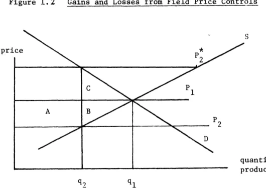
-28-Figure 1.2 Gains and Losses from Field Price Controls
S
uantity
rN1l c1l
-hypothetical unregulated comsumption at constant reserve backing multiplied by (b) the difference between the unregulaed and the "shadow" price (that
33 would clear the market of regulated demand at constant reserve backing).
Field producers experience losses from price ceilings as a matter of course. They lose by price ceilings those amounts gained by consumers on established service, and also lose roughly an amount equal to one-half the difference between regulated and unregulated prices times the difference between regulated and unregulated production.
Any estimates of these price and quantity differences is most inexact, particularly because they depend on "unregulated" prices, when regulation throughout the decade has prevented observations of any such prices. Also, any overall assessment depends upon whether the gains to established
con-33
This can be seen by inspection of the rudimentary supply-demand diagram, in Figure 1.1, as follows: the gains of established consumers are repre-sented by Area A and the losses of consumers with reduced backing is shown by Area C.
The statement on prices in the text can be understood by inspection of the diagram. Here ql and q2 are at the old reserve production ratio (since
otherwise measurements of gains and losses would be made while "quality
of service" in reserve backing was also being allowed to vary). The measures used here are the levels of production implied by constant R/p ratios shown in Table 1.3 The estimates for ql are given by production at hypothetical "unregulated" field prices (Column 2) and for q2 by production at regulated
prices at constant R/P ratio (Column 1). The price appropriate for regu-lated q2 is P*2 which clears the market of the reduced quantity q2
(result-ing from the freeze at P2). This price P 2 has been estimated by simulation
with the econometric model.
There is also a loss by producers equal to Areas A and B. Again, these are measured at the mid-1960's constant R/p ratio, and thus are the same ql and q2 as in the last paragraph. The net losses to all groups combined
are equal to Areas B plus C, unless specific weightings are assigned to the "worth" of a dollar taken away from producers and a dollar given to consumers. Such a specific weighting of, say, 0.0 on the first and 1.0 on the second would attribute Area A to net economy-wide gains. No such attribution is made here.
3 4
This is the number of dollars equivalent to Area B in the diagram in the preceding footnote.
-30-sumers are treated as worth more than the losses of producers. Neverthe-less, as an indication of the orders of magnitude of gains from the price controls, estimates of prices and quantities have been made from simulations with the econometric model. Field prices are as under regulation or, alter-natively, at the simulated "unregulated" levels shown as being necessary
to preserve the reserve backing. Alternative levels of production are as simulated at actual prices at a constant R/P ratio, or as simulated at hypothetical unregulated prices.35 From these prices and quantities, the gains and losses have been estimated as follows:
(1) Gains to Consumers (Area A) billions of dollars 0.3 0.7 1.2 1.7 2.2 2.5 (2) Losses to Consumers from a Reduction in Reserve Backing (Area C) billions of dollars 0.0 0.1 0.1
0.1
0.1
0.1 Losses to Producers (3) (4) (Area A) (Area ];) billions of dollars 0.3 0.0 0.7 0.1 1.2 0.1 1.7 0.1 2.2 0.1 2.5 0.1 3 4This is the number of dollars equivalent to Area B in the diagram in the preceding footnote.
35
The two simulation series for quantities are as shown in Table 1.3 as Columns (1) and (2) respectively. The Column (1) series is correct for regulated prices because it shows the amount of production at the "same" or constant R/P ratio. This amount is the proper level on which to assess gains of established consumers, since no reserve backing has been lost to that point. This takes account of net benefits after adjustment has been made for the losses to consumers from the elimination of reserve backing. The calculations of Areas A, B, and C are based on the assumption that the loss of reserve backing was equivalent to the reduction of present tion at constant reserve backing, and that that reduction of present consump-tion is equivalent to the lowest level of producconsump-tion q2 in the diagram
above. Year 1967 1968 1969 1970 1971 1972
-These are "static" gains and losses) since they include only one year's production results.3 6 As limited as they are, they show that con-sumers as a group gained. What they gained, producers lost. The losses which would have gone into dividends to stockholders of gas companies, or into new investment in exploration and development, cannot be ignored entirely even if they were recognized by the regulatory commission. All that can be said is that the price freeze did more good for buyers in holding down their monthly payments of gas bills than the losses to them from reductions in reserves, and that the freeze did slightly more harm to producers in income and production losses.37
Whether this array of benefits and costs from field price controls will continue. in the 1970's is the concern of the next chapter. During the later 1970's, the shortage of production consequent-upon the reduced reserve backing should by itself lead to greater losses to established customers. An attempt is made in the next chapter to show whether there will still be net gains from regulation to customers then--particularly to interstate customers (since they are being protected by the Federal Power Commission from price increases).
1.4. Summary
The Federal Power Commission, having been given tle task of regulating gas field prices by the Supreme Court, tried any number of ways of adapting old
regulatory techniques to new contracts for producing gas reserves. The rationale for regulation provided by the courts centered on keeping prices
3 6
Because of the extreme imprecision of the basis for estimates, a more complex dynamic analysis was ruled out at this point. Nor would the general results be further illuminated by discounting these numbers to present value at the time of the temporary area rates.
That is, the sum of consumer gains (Areas A-C) falls slightly short of producer losses (Areas A+B).
-32-at the levels experienced in the l-32-ate 1950's; prices were to be stabilized for stability's sake. The Commission's resolve to hold the price level was strengthened by court decisions stressing that the FPC could set
prices using whatever review process seemed most appropriate. Eventually, in the area rate proceedings, the FPC found the means for invoking freezes on prices over wide regions.
There is little question but that price stability was achieved. Stability probably led to deficiencies in supplies of reserves and, ulti-mately, deficiencies in production of gas in the early 1970's (as shown by simulations with the MIT econometric model described below. In the absence of controls, prices probably would have gone up enough to have maintained at least a fifteen--to-one reserve production ratio, and to have held back demands'so as co have cleared field markets of all new reserve demands. Model simulations based on these conditions show that
higher "unregulated" prices (sufficient to have cleared reserve markets)would have dampened demands and would have been at best 60 percent higher on new
contracts, and when such prices were rolled in to wholesale changes, resi-dential and commercial customers would have paid 20 percent more for the amounts they actually consumed.
To some extent, given these conclusions, the rationale for regulation can be judged in retrospect. Even though the courts and Commission are not explicit on who should receive the benefits from regulation, it might be assumed that those who actually did benefit were meant to be blessed by
the regulatory process. Assuming such does not lead to a very clear and consistent view of regulation. Consumers, particularly in the South outside of FPC controls benefited from low prices on the production they received. But they and others lost their reserve backing, since old reserves were used to provide for expanded production for new consumers--indeed into the
market by relatively low frozen prices. The model simulations of benefits and losses for particular groups indicate that consumers as a whole
received benefits from lower regulated prices, even after accounting for losses for some from reduced reserve backing, and producers as a whole
experienced losses to a somewhat greater extent than the consumers gained. Thus up to the beginning of the production shortage consumers at least may have benefited from controls. The rationale for regulation may have been no more than that of income redistribution to gas customers up to the point of production shortage. The rationale for the production