HAL Id: obspm-02268051
https://hal-obspm.ccsd.cnrs.fr/obspm-02268051
Submitted on 19 Jan 2021
HAL is a multi-disciplinary open access
archive for the deposit and dissemination of
sci-entific research documents, whether they are
pub-lished or not. The documents may come from
teaching and research institutions in France or
abroad, or from public or private research centers.
L’archive ouverte pluridisciplinaire HAL, est
destinée au dépôt et à la diffusion de documents
scientifiques de niveau recherche, publiés ou non,
émanant des établissements d’enseignement et de
recherche français ou étrangers, des laboratoires
publics ou privés.
HARPS-N high spectral resolution observations of
Cepheids I. The Baade-Wesselink projection factor of δ
Cep revisited
N. Nardetto, E. Poretti, M. Rainer, A. Fokin, P. Mathias, R. Anderson, A.
Gallenne, W. Gieren, D. Graczyk, P. Kervella, et al.
To cite this version:
N. Nardetto, E. Poretti, M. Rainer, A. Fokin, P. Mathias, et al.. HARPS-N high spectral resolution
observations of Cepheids I. The Baade-Wesselink projection factor of δ Cep revisited. Astronomy
and Astrophysics - A&A, EDP Sciences, 2017, 597, pp.A73. �10.1051/0004-6361/201629400�.
�obspm-02268051�
DOI:10.1051/0004-6361/201629400 c ESO 2017
Astronomy
&
Astrophysics
HARPS-N high spectral resolution observations of Cepheids
I. The Baade-Wesselink projection factor of
δ
Cep revisited
?
N. Nardetto
1, E. Poretti
2, M. Rainer
2, A. Fokin
3, P. Mathias
4,5, R. I. Anderson
6, A. Gallenne
7,8, W. Gieren
8,9,
D. Graczyk
8,9,10, P. Kervella
11,12, A. Mérand
7, D. Mourard
1, H. Neilson
13, G. Pietrzynski
10,
B. Pilecki
10, and J. Storm
141 Université Côte d’Azur, OCA, CNRS, Lagrange, France
e-mail: Nicolas.Nardetto@oca.eu
2 INAF–Osservatorio Astronomico di Brera, via E. Bianchi 46, 23807 Merate (LC), Italy
3 Institute of Astronomy of the Russian Academy of Sciences, 48 Pjatnitskaya Str., 109017 Moscow, Russia
4 Université de Toulouse, UPS-OMP, Institut de Recherche en Astrophysique et Planétologie, 31400 Toulouse, France
5 CNRS, UMR 5277, Institut de Recherche en Astrophysique et Planétologie, 14 avenue Édouard Belin, 31400 Toulouse, France 6 Department of Physics and Astronomy, The Johns Hopkins University, 3400 N. Charles St, Baltimore, MD 21218, USA 7 European Southern Observatory, Alonso de Córdova 3107, Casilla 19001, Santiago 19, Chile
8 Departamento de Astronomía, Universidad de Concepción, Casilla 160-C, Concepción, Chile 9 Millenium Institute of Astrophysics, Santiago, Chile
10 Nicolaus Copernicus Astronomical Center, Polish Academy of Sciences, ul. Bartycka 18, 00-716 Warszawa, Poland
11 LESIA (UMR 8109), Observatoire de Paris, PSL, CNRS, UPMC, Univ. Paris-Diderot, 5 place Jules Janssen, 92195 Meudon,
France
12 Unidad Mixta Internacional Franco-Chilena de Astronomía, CNRS/INSU, France (UMI 3386) and Departamento de Astronomía,
Universidad de Chile, Camino El Observatorio 1515, Las Condes, Santiago, Chile
13 Department of Astronomy & Astrophysics, University of Toronto, 50 St. George Street, Toronto, ON, M5S 3H4, Canada 14 Leibniz Institute for Astrophysics, An der Sternwarte 16, 14482 Potsdam, Germany
Received 26 July 2016/ Accepted 21 October 2016
ABSTRACT
Context.The projection factor p is the key quantity used in the Baade-Wesselink (BW) method for distance determination; it converts
radial velocities into pulsation velocities. Several methods are used to determine p, such as geometrical and hydrodynamical models or the inverse BW approach when the distance is known.
Aims.We analyze new HARPS-N spectra of δ Cep to measure its cycle-averaged atmospheric velocity gradient in order to better
constrain the projection factor.
Methods.We first apply the inverse BW method to derive p directly from observations. The projection factor can be divided into
three subconcepts: (1) a geometrical effect (p0); (2) the velocity gradient within the atmosphere ( fgrad); and (3) the relative motion of
the optical pulsating photosphere with respect to the corresponding mass elements ( fo−g). We then measure the fgradvalue of δ Cep
for the first time.
Results.When the HARPS-N mean cross-correlated line-profiles are fitted with a Gaussian profile, the projection factor is pcc−g =
1.239 ± 0.034(stat.) ± 0.023(syst.). When we consider the different amplitudes of the radial velocity curves that are associated with 17 selected spectral lines, we measure projection factors ranging from 1.273 to 1.329. We find a relation between fgradand the line
depth measured when the Cepheid is at minimum radius. This relation is consistent with that obtained from our best hydrodynamical model of δ Cep and with our projection factor decomposition. Using the observational values of p and fgradfound for the 17 spectral
lines, we derive a semi-theoretical value of fo−g. We alternatively obtain fo−g= 0.975 ± 0.002 or 1.006 ± 0.002 assuming models using
radiative transfer in plane-parallel or spherically symmetric geometries, respectively.
Conclusions.The new HARPS-N observations of δ Cep are consistent with our decomposition of the projection factor. The next step
will be to measure p0directly from the next generation of visible interferometers. With these values in hand, it will be possible to
derive fo−gdirectly from observations.
Key words. stars: oscillations – techniques: spectroscopic – stars: individual: delta Cep – stars: distances – stars: atmospheres –
stars: variables: Cepheids
1. Introduction
Since their period-luminosity (PL) relation was established (Leavitt & Pickering 1912), Cepheid variable stars have been used to calibrate the distance scale (Hertzsprung 1913) and then
? Table A.1 is also available at the CDS via anonymous ftp to
cdsarc.u-strasbg.fr(130.79.128.5) or via
http://cdsarc.u-strasbg.fr/viz-bin/qcat?J/A+A/597/A73
the Hubble constant (Riess et al. 2011; Freedman et al. 2012; Riess et al. 2016). The discovery that the K-band PL relation is nearly universal and can be applied to any host galaxy what-ever its metallicity (Storm et al. 2011a) is a considerable step forward in the use of Cepheids as distance indicators. Deter-mining the distances to Cepheids relies on the Baade-Wesselink (BW) method, which in turn relies on a correct evaluation of the projection factor p. This is necessary to convert the radial
Table 1. Non-exhaustive history of the determination of the Baade-Wesselink projection factor in the case of δ Cep.
Method p Reference
Geometrical models
Centroid 1.415 Getting(1934)
Centroid 1.375 van Hoof & Deurinck(1952) Centroid 1.360 Burki et al.(1982)
Centroid 1.328 Neilson et al.(2012) Hydrodynamical models
Bisector 1.34 Sabbey et al.(1995) Gaussian 1.27 ± 0.01 Nardetto et al.(2004) cc-g (Pp) 1.25 ± 0.05 Nardetto et al.(2009) Observations cc-g 1.273 ± 0.021 ± 0.050 Mérand et al.(2005) cc-g 1.245 ± 0.030 ± 0.050 Groenewegen(2007) cc-g 1.290 ± 0.020 ± 0.050 Merand et al.(2015) cc-g (Pp) 1.47 ± 0.05 Gieren et al.(2005b) cc-g (Pp) 1.29 ± 0.06 Laney & Joner(2009) cc-g (Pp) 1.41 ± 0.05 Storm et al.(2011b) cc-g (Pp) 1.325 ± 0.03 Groenewegen(2013)
Notes. The method used to derive the radial velocity is indicated, and cc-g corresponds to a Gaussian fit of the cross-correlated line profile. For the values of the projection factor derived from a published period projection factor relation, we consistently use a period of P= 5.366208 days (Engle et al. 2014).
velocity variations derived from the spectral line profiles into photospheric pulsation velocities (Nardetto et al. 2004).
The projection factor of δ Cep, the eponym of the Cepheid variables, has been determined by means of different techniques, which we summarize here (see Table1and the previous review byNardetto et al. 2014b):
– Purely geometric considerations lead to the identification of two contributing effects only in the projection factor, i.e., the limb darkening of the star and the motion (expansion or contraction) of the atmosphere.Nardetto et al. (2014b) de-scribed this classical approach and its recent variations (e.g., Gray & Stevenson 2007;Hadrava et al. 2009).
– To improve the previous method we should consider that Cepheids do not pulsate in a quasi-hydrostatic way and the dynamical structure of their atmosphere is extremely complex (Sanford 1956; Bell & Rodgers 1964;Karp 1975; Sasselov & Lester 1990;Wallerstein et al. 2015). Therefore, improving the determination of the BW projection factor requires a hydrodynamical model that is able to describe the atmosphere. To date, the projection factor has been studied with two such models: the first is based on a pis-ton in which the radial velocity curve is used as an in-put (Sabbey et al. 1995) and the second is a self-consistent model (Nardetto et al. 2004). Sabbey et al.(1995) found a mean value of the projection factor p = 1.34 (see also Marengo et al. 2002,2003). However, this value was derived using the bisector method of the radial velocity determina-tion (applied to the theoretical line profiles). This makes it difficult to compare this value with other studies. As com-monly done in the literature, if a Gaussian fit of the cross-correlated line-profile is used to derive the radial velocity RVcc−g(“cc” for cross-correlated and “g” for Gaussian), then
the measured projection factor tends to be about 11% smaller than the initial geometrical projection factor is found, i.e., p= 1.25 ± 0.05 (Nardetto et al. 2009).
– As an approach entirely based on observations,Mérand et al. (2005) applied the inverse BW method to infrared inter-ferometric data of δ Cep. The projection factor is then fit, where the distance of δ Cep is known with 4% uncertainty from the HST parallax (d = 274 ± 11 pc; Benedict et al. 2002). They found p= 1.273 ± 0.021 ± 0.050 using RVcc−g
for the radial velocity. The first error is the internal one due to the fitting method. The second is due to the un-certainty of the distance. Groenewegen (2007) found p = 1.245 ± 0.030 ± 0.050 when using almost the same dis-tance (273 instead of 274 pc), a different radial velocity dataset and a different fitting method of the radial velocity curve. Recently,Merand et al. (2015) applied an integrated inverse method (SPIPS) to δ Cep (by combining interferom-etry and photominterferom-etry) and found p = 1.29 ± 0.02 ± 0.05. These values agree closely with the self-consistent hydrody-namical model. Another slightly different approach is to ap-ply the infrared surface brightness inverse method to distant Cepheids (seeFouque & Gieren 1997;Kervella et al. 2004a, for the principles) in order to derive a period projection fac-tor relation (Pp). In this approach the distance to each LMC Cepheid is assumed to be the same by taking into account the geometry of LMC. This constrains the slope of the Pp rela-tion. However, its zero-point is alternatively fixed using dis-tances to Cepheids in Galactic clusters (Gieren et al. 2005b), HST parallaxes of nearby Cepheids derived by van Leeuwen et al. (2007;Laney & Joner 2009;Storm et al. 2011b), or a combination of both (Groenewegen 2013). Laney & Joner (2009) also used high-amplitude δ Scuti stars to derive their Pp relation (see also Fig. 10 inNardetto et al. 2014a). The projection factors derived byLaney & Joner(2009) and Groenewegen (2013) are consistent with the interferomet-ric values, while the projection factors from Gieren et al. (2005b) and Storm et al. (2011b) are significantly greater (see Table1).
– Pilecki et al.(2013) constrained the projection factor using a short-period Cepheid (P = 3.80 d, similar to the pe-riod of δ Cep) in a eclipsing binary system. They found p= 1.21 ± 0.04.
This non-exhaustive review shows just how complex the situa-tion regarding the value of the BW projecsitua-tion factor of δ Cep is. This paper is part of the international “Araucaria Project”, whose purpose is to provide an improved local calibration of the extragalactic distance scale out to distances of a few megaparsecs (Gieren et al. 2005a). In Sect. 2 we present new High Accuracy Radial velocity Planet Searcher for the North-ern hemisphere (HARPS-N) observations. Using these spec-tra together with the Mérand et al. (2005) data obtained with the Fiber Linked Unit for Optical Recombination (FLUOR, Coudé du Foresto et al. 1997) operating at the focus of the Cen-ter for High Angular Resolution Astronomy (CHARA) array (ten Brummelaar et al. 2005) located at the Mount Wilson Ob-servatory (California, USA), we apply the inverse BW method to derive the projection factor associated with the RVcc−g
ra-dial velocity and for 17 individual spectral lines (Sect. 3). In Sect. 4, we briefly describe the hydrodynamical model used in Nardetto et al. (2004) and review the projection factor decom-position into three sub-concepts (p= p0fgradfo−g,Nardetto et al.
2007). In Sect.4.1, we compare the observational and theoretical projection factors. We then compare the hydrodynamical model with the observed atmospheric velocity gradient (Sect.4.2) and the angular diameter curve of FLUOR/CHARA (Sect. 4.3). In Sect. 5we derive the fo−g quantity from the previous sections.
We conclude in Sect.6.
2. HARPS-N spectroscopic observations
HARPS-N is a high-precision radial-velocity spectrograph in-stalled at the Italian Telescopio Nazionale Galileo (TNG), a 3.58-m telescope located at the Roque de los Muchachos Ob-servatory on the island of La Palma, Canary Islands, Spain (Cosentino et al. 2012). HARPS-N is the northern hemisphere counterpart of the similar HARPS instrument installed at the ESO 3.6 m telescope at La Silla Observatory in Chile. The in-strument covers the wavelength range from 3800 to 6900 Å with a resolving power of R ' 115 000. A total of 103 spectra were secured between 27 March and 6 September 2015 in the frame-work of the OPTICON proposal 2015B/015 (TableA.1). In or-der to calculate the pulsation phase of each spectrum, we used P = 5.366208 d (Engle et al. 2014) and T0 = 2 457 105.930 d,
the time corresponding to the maximum approaching veloc-ity determined from the HARPS-N radial velocities. The data are spread over 14 of the 30 pulsation cycles elapsed between the first and last epoch. The final products of the HARPS-N data reduction software (DRS) installed at TNG (on-line mode) are background-subtracted, cosmic-corrected, flat-fielded, and wavelength-calibrated spectra (with and without merging of the spectral orders). We used these spectra to compute the mean-line profiles by means of the least-squares deconvolution (LSD) technique (Donati et al. 1997). As can be seen in Fig.1, the mean profiles reflect the large-amplitude radial pulsation by distorting the shape in a continuous way.
The DRS also computes the star’s radial velocity by fitting a Gaussian function to the cross-correlation functions (CCFs). To do this, the DRS uses a mask including thousands of lines covering the whole HARPS-N spectral ranges. The observer can select the mask among those available online and the G2
Fig. 1.Mean line profile changes during the pulsation cycle of δ Cep. The line profile with the highest receding motion is highlighted in red, the one with the highest approaching motion in blue.
mask was the closest to the δ Cep spectral type. As a further step, we re-computed the RV values by using the HARPS-N DRS in the offline mode on the Yabi platform, as in the case of τ Boo (Borsa et al. 2015). We applied both library and cus-tom masks, ranging spectral types from F5 to G2. We obtained RV curves fitted with very similar sets of least-squares param-eters showing only some small changes in the mean values. TableA.1lists the RVcc−gvalues obtained from the custom F5I
mask, also plotted in panel a) of Fig.2 with different symbols for each pulsation cycle. The RV curve shows a full amplitude of 38.4 km s−1 and an average value (i.e., the A0value of the fit)
of Vγ = −16.95 km s−1. As a comparison, we calculate the cen-troid of the mean line profiles RVcc−c(“cc” for cross-correlated
and “c” for centroid) and plot the residuals in panel b) of Fig.2. The RVcc−ccurve has an amplitude 1.2 km s−1 lower than that of
the RVcc−gvalue. This result is similar to that reported in the case
of β Dor (Fig. 2 in Nardetto et al. 2006). The implications of this difference on the projection factor is discussed in Sect.3.1.
Consistent withAnderson et al.(2015), we find no evidence for cycle-to-cycle differences in the RV amplitude as exhib-ited by long-period Cepheids (Anderson 2014; Anderson et al. 2016). We also investigated the possible effect of the binary mo-tion due to the companion (Anderson et al. 2015). Unfortunately, the HARPS-N observations are placed on the slow decline of the RV curve and they only span 160 days. We were able to detect a slow drift of −0.5 ± 0.1 m s−1d−1. The least-squares solution
with 14 harmonics leaves a r.m.s. residual of 49 m s−1. Includ-ing a linear trend did not significantly reduce the residual since the major source of error probably lies in the fits of the very dif-ferent shapes of the mean-line profiles along the pulsation cycle (Fig.1). We also note that surface effects induced by convection and granulation (Neilson & Ignace 2014) could contribute to in-creasing the residual r.m.s. These effects are also observed in the light curves of Cepheids (Derekas et al. 2012,2017;Evans et al. 2015;Poretti et al. 2015).
-20 -10 0 10 20
cross-correlated radial velocity (km/s)
a) RVcc-g (F5I) cycle 0 cycle 1 cycle 5 cycle 6 cycle 7 cycle 8 cycle 9 cycle 10 cycle 11 cycle 12 cycle 13 cycle 18 cycle 19 cycle 27 cycle 30 -2 -1.5 -1 -0.5 0 0.5 1 1.5 2 0 0.2 0.4 0.6 0.8 1 1.2 km/s pulsation phase b) RVcc-c (F5I) - RVcc-g (F5I)
Fig. 2. Panel a): HARPS-N radial veloci-ties associated with the Gaussian fit of the cross-correlated line profile (RVcc−g using F5I
template) plotted as a function of the pulsa-tion phase of the star after correcpulsa-tion of the γ-velocity (i.e., Vγ= −16.95 km s−1). The cy-cle of observations are shown in different col-ors. The data are reproduced from one cycle to the other. The precision on the measure-ments is between 0.5 and 1.5 m s−1(error bars
are lower than symbols). Panel b) residuals be-tween RVcc−c(F5I) and RVcc−g(F5I) after
cor-rection of their respective γ-velocities.
3. Inverse Baade-Wesselink projection factors derived from observations
3.1. Using the cross-correlated radial velocity curve
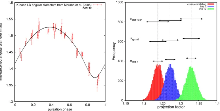
We describe the interferometric version of the BW method as follows. We apply a classical χ2minimization
χ2=X i (θobs(φi) − θmodel(φi))2 σobs(φi)2 , (1) where
– θobs(φi) are the interferometric limb-darkened angular
diameters obtained from FLUOR/CHARA observations (Mérand et al. 2005), with φithe pulsation phase
correspond-ing to the ith measurement (Fig.3);
– σobs(φi) are the statistical uncertainties corresponding to
FLUOR/CHARA measurements;
– θmodel(φi) are the modeled limb-darkened angular diameters,
defined as θmodel(φi)= θ + 9.3009 pcc−g d Z RVcc−g(φi)dφi ! [mas], (2) where the conversion factor 9.3009 is defined using the solar radius given inPrša et al.(2016).
The RVcc−g(φi) is the interpolated HARPS-N
cross-correlated radial velocity curve shown in panel a) of Fig.2. It is obtained using the Gaussian fit, i.e., the most common approach in the literature. The parameters θ and pcc−gare the mean angular
diameter of the star (in mas) and the projection factor (associated
with the Gaussian fit of the CCFs), respectively, while d is the distance to the star. The quantities θ and pcc−gare fit in order to
minimize χ2, while d is fixed to d= 272 ± 3(stat.) ± 5(syst.) pc
(Majaess et al. 2012).
We find θ = 1.466 ± 0.007 mas and pcc−g = 1.239 ±
0.031, where the uncertainty on the projection factor (here-after σstat−fluor) is about 2.5% and stems from FLUOR/CHARA
angular diameter measurements. If we apply this procedure 10 000 times using a Gaussian distribution for the assumed dis-tance that is centered at 272 pc and has a half width at half max-imum (HWHM) of 3 pc (corresponding to the statistical pre-cision on the distance of Majaess et al. 2012), then we obtain a symmetric distribution for the 10 000 values of pcc−g with a
HWHM σstat−d = 0.014. If the distance is set to 277 pc and
267 pc (corresponding to the systematical uncertainty of ±5 pc of Majaess et al. 2012), we find p= 1.262 and p = 1.216, respec-tively. We have a systematical uncertainty σsyst−d= 0.023 for the
projection factor. We thus find pcc−g= 1.239 ± 0.031 (σstat−fluor)
±0.014 (σstat−d) ±0.023 (σsyst−d). These results are illustrated in
Fig.4. Interestingly, if we use the RVcc−ccurve in Eq. (2) (still
keeping d = 272 pc), we obtain pcc−c = 1.272 while the
uncer-tainties remain unchanged.
The distance of δ Cep obtained by Majaess et al. (2012) is an average of H
ipparcos
(van Leeuwen 2007) and HST (Benedict et al. 2002) trigonometric parallaxes, together with the cluster main sequence fitting distance. If we rely on the direct distance to δ Cep obtained only by HST (Benedict et al. 2002), i.e., 273 ± 11 pc, then σstat−dis larger with a value of 0.050(com-pared to 0.014 when relying onMajaess et al. 2012). A distance d = 244 ± 10 pc was obtained byAnderson et al.(2015) from
1.3 1.35 1.4 1.45 1.5 1.55 1.6 0 0.2 0.4 0.6 0.8 1
limb-darkened angular diameter (mas)
pulsation phase
K-band LD angular diameters from Merand et al. (2005) best fit
Fig. 3. Inverse BW method applied to FLUOR/CHARA data (Mérand et al. 2005) considering a distance for δ Cep of d = 272 ± 3 ± 5 pc (Majaess et al. 2012) and the HARPS-N cross-correlated radial velocity curve. The black dotted line corresponds to the best fit. Table 2. Spectral lines used this study.
No. El. Wavelength (Å) E p(eV) log(g f )
1 Fe
i
4683.560 2.831 –2.319 2 Fei
4896.439 3.883 –2.050 3 Nii
5082.339 3.658 –0.540 4 Fei
5367.467 4.415 0.443 5 Fei
5373.709 4.473 –0.860 6 Fei
5383.369 4.312 0.645 7 Tiii
5418.751 1.582 –2.110 8 Fei
5576.089 3.430 –1.000 9 Fei
5862.353 4.549 –0.058 10 Fei
6003.012 3.881 –1.120 11 Fei
6024.058 4.548 –0.120 12 Fei
6027.051 4.076 –1.089 13 Fei
6056.005 4.733 –0.460 14 Sii
6155.134 5.619 –0.400 15 Fei
6252.555 2.404 –1.687 16 Fei
6265.134 2.176 –2.550 17 Fei
6336.824 3.686 –0.856the reanalysis of the H
ipparcos
astrometry of δ Cep. It leads to a very small projection factor pcc−g = 1.14 ± 0.031 ± 0.047compared to other values listed in Table1.
3.2. Using the first moment radial velocity curves corresponding to individual spectral lines
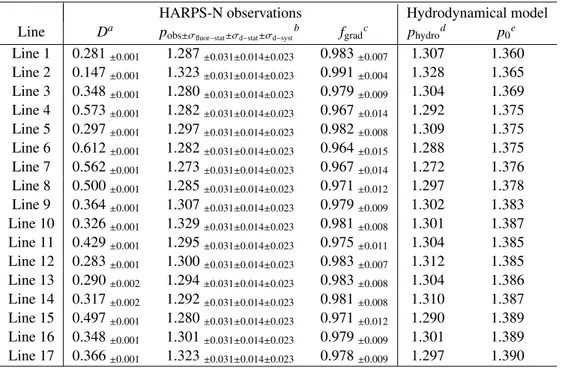
We use the 17 unblended spectral lines (Table2) that were pre-viously selected for an analysis of eight Cepheids with periods
0 200 400 600 800 1000 1.15 1.2 1.25 1.3 1.35 1.4 Frequency projection factor σstat-d σstat-fluor σ syst-d cross-correlation line 7 line 10
Fig. 4.Inverse BW method described in Sect.3applied considering a Gaussian distribution for the distance. The resulting projection fac-tor distributions are shown in three particular cases: when using the cross-correlated radial velocity curve RVcc−g (red), the RVcradial
ve-locity curve of line 7 (blue), and the RVcradial velocity curve of line
10 (green). The quantities σstat−d and σsyst−d are the uncertainties on
the projection factor due to the statistical and systematical uncertain-ties on the distance, respectively. The quantity σstat−fluorstems from the
statistical uncertainties on the FLUOR/CHARA interferometric mea-surements.
ranging from 4.7 to 42.9 d (Nardetto et al. 2007). These lines re-main unblended for every pulsation phase of the Cepheids con-sidered. Moreover, they were carefully selected in order to rep-resent a wide range of depths, hence to measure the atmospheric velocity gradient (Sect.4.2). For each of these lines, we derive the centroid velocity (RVc), i.e., the first moment of the spectral
line profile, estimated as
RVc= R lineλS (λ)dλ R lineS(λ)dλ , (3)
where S (λ) is the observed line profile. The radial velocity mea-surements associated with the spectral lines are presented in Fig. 5a together with the interpolated RVcc−g curve. The RVc
curves plotted have been corrected for the γ-velocity value cor-responding to the RVcc−g curve, i.e., Vγ = −16.95 km s−1.
The residuals, i.e., the γ-velocity offsets, between the curves of Fig.5a are related to the line asymmetry and the k-term value (seeNardetto et al. 2008, for Cepheids; andNardetto et al. 2013, 2014a, for other types of pulsating stars). This will be analyzed in a forthcoming paper. The final RVccurves used in the inverse
BW approach are corrected from their own residual γ-velocity in such a way that the interpolated curve has an average of zero. The residual of these curves compared to the RVcc−gand RVcc−c
curves are shown in panel b and c, respectively. We then apply the same method as in Sect.3.1. The measured projection fac-tor values pobs(k) associated with each spectral line k are listed
-25 -20 -15 -10 -5 0 5 10 15 20 25
first moment radial velocity curves (km/s)
a) line 1 line 2 line 3 line 4 line 5 line 6 line 7 line 8 line 9 line 10 line 11 line 12 line 13 line 14 line 15 line 16 line 17 -5 -4 -3 -2 -1 0 1 2 3 4 5 km/s b) -5 -4 -3 -2 -1 0 1 2 3 4 5 0 0.2 0.4 0.6 0.8 1 1.2 km/s pulsation phase c)
Fig. 5. a) First moment radial velocity curves (RVc) associated with the 17 lines of
Table 2. The γ-velocity associated with the cross-correlated radial velocity curve, RVcc−gin
Fig. 2a, has been removed from these curves, i.e., Vγ = −16.95 km s−1. The γ offset
resid-uals are known to be related to the k-term (Nardetto et al. 2008). The residuals between the RVccurves and the RVcc−gin Fig.2a (resp.
RVcc−c) are plotted in panel b) (resp. c)) after
correcting each RVccurve from its Vγvalue.
case of individual lines are the same as those found when using the RVcc−gcurve. The projection factor values range from 1.273
(line 7) to 1.329 (line 10), whereas the value corresponding to the cross-correlation method is 1.239 (see Fig.4). This shows that the projection factor depends significantly on the method used to derive the radial velocity and the spectral line considered. To analyze these values it is possible to use hydrodynamical simu-lations and the projection factor decomposition into three terms introduced byNardetto et al.(2007).
4. Comparing the hydrodynamical model of
δ
Cepwith observations
Our best model of δ Cep was presented inNardetto et al.(2004) and is computed using the code by Fokin(1991). The hydro-dynamical model requires only five input fundamental parame-ters: M = 4.8 M , L= 1995 L , Teff = 5877 K, Y = 0.28, and
Z= 0.02. At the limit cycle the pulsation period is 5.419 d, very close (1%) to the observed value.
4.1. Baade-Wesselink projection factors derived from the hydrodynamical model
The projection factors are derived directly from the hydrody-namical code for each spectral line of Table 2 following the definition and procedure described in Nardetto et al. (2007). The computed projection factors range from 1.272 (line 7) to 1.328 (line 2). In Fig.6we plot the theoretical projection fac-tors (phydro) as a function of the observational values (listed in
Table3). In this figure the statistical uncertainties on the obser-vational projection factors, i.e., σstat−fluorand σstat−d, have been
summed quadratically (i.e., σ = 0.034). The agreement is ex-cellent since the most discrepant lines (10 and 17, in red in the figure) show observational projection factor values only about 1σ larger than the theoretical values.
4.2. Atmospheric velocity gradient ofδ Cep
In Nardetto et al. (2007), we split the projection factor into three quantities: p = po fgradfo−g, where p0 is the geometrical
Table 3. The observational quantities, D, pobs, and fgrad, are listed for each line of Table2.
HARPS-N observations Hydrodynamical model
Line Da p
obs±σfluor−stat±σd−stat±σd−syst
b f gradc phydrod p0e Line 1 0.281±0.001 1.287±0.031±0.014±0.023 0.983±0.007 1.307 1.360 Line 2 0.147±0.001 1.323±0.031±0.014±0.023 0.991±0.004 1.328 1.365 Line 3 0.348±0.001 1.280±0.031±0.014±0.023 0.979±0.009 1.304 1.369 Line 4 0.573±0.001 1.282±0.031±0.014±0.023 0.967±0.014 1.292 1.375 Line 5 0.297±0.001 1.297±0.031±0.014±0.023 0.982±0.008 1.309 1.375 Line 6 0.612±0.001 1.282±0.031±0.014±0.023 0.964±0.015 1.288 1.375 Line 7 0.562±0.001 1.273±0.031±0.014±0.023 0.967±0.014 1.272 1.376 Line 8 0.500±0.001 1.285±0.031±0.014±0.023 0.971±0.012 1.297 1.378 Line 9 0.364±0.001 1.307±0.031±0.014±0.023 0.979±0.009 1.302 1.383 Line 10 0.326±0.001 1.329±0.031±0.014±0.023 0.981±0.008 1.301 1.387 Line 11 0.429±0.001 1.295±0.031±0.014±0.023 0.975±0.011 1.304 1.385 Line 12 0.283±0.001 1.300±0.031±0.014±0.023 0.983±0.007 1.312 1.385 Line 13 0.290±0.002 1.294±0.031±0.014±0.023 0.983±0.008 1.304 1.386 Line 14 0.317±0.002 1.292±0.031±0.014±0.023 0.981±0.008 1.310 1.387 Line 15 0.497±0.001 1.280±0.031±0.014±0.023 0.971±0.012 1.290 1.389 Line 16 0.348±0.001 1.301±0.031±0.014±0.023 0.979±0.009 1.301 1.389 Line 17 0.366±0.001 1.323±0.031±0.014±0.023 0.978±0.009 1.297 1.390
Notes. The quantities phydro, p0and fo−gare derived from hydrodynamical model.(a)The line depth D is calculated at minimum radius of the
star. (b) The observational projection factors p
obs is derived from HARPS-N and FLUOR/CHARA interferometric data using the inverse BW
approach (Sect.3.2). (c)The f
grad coefficient involved in the projection factor decomposition (p = p0fgradfo−g,Nardetto et al. 2007) is derived
from Eqs.5and6(Sect.4.2). (d)The inverse projection factors p
hydrois calculated with the hydrodynamical model (Sect.4.1). (e)The modeled
geometric projection factor p0is derived in the continuum next to each spectral line. The fo−gquantity, which is obtained using the projection
factor decomposition ( fo−g= pobs
pofgrad), is derived in Sect.5.
1.24 1.26 1.28 1.3 1.32 1.34 1.36 1.24 1.26 1.28 1.3 1.32 1.34 1.36
projection factor from observations
projection factor from theory line 1 line 2 line 3 line 4 line 5 line 6 line 7 line 8 line 9 line 10 line 11 line 12 line 13 line 14 line 15 line 16 line 17
Fig. 6.Observational projection factors derived using the inverse BW approach described in Sect.3compared to the theoretical values ob-tained from the hydrodynamical model (Sect.4.1).
projection factor (linked to the limb darkening of the star); fgrad,
which is a cycle-integrated quantity linked to the velocity gra-dient in the atmosphere of the star (i.e., between the considered
line-forming region and the photosphere); and fo−g, which is the
relative motion of the optical pulsating photosphere with respect to the corresponding mass elements.
We derive fgrad directly from HARPS-N observations. In
Nardetto et al.(2007), we showed that the line depth taken at the minimum radius phase (hereafter D) traces the height of the line-forming regions in such a way that the projection factor decom-position is possible. By comparing∆RVcwith the depth, D, of
the 17 selected spectral lines listed in Table2, we directly mea-sure fgrad. If we define a0 and b0 as the slope and zero-point of
the linear correlation (the photosphere being the zero line depth),
∆RVc= a0D+ b0, (4)
then the velocity gradient correction on the projection factor is fgrad=
b0
a0D+ b0
· (5)
InAnderson(2016) the atmospheric velocity gradient is defined as the difference between velocities determined using weak and strong lines at each pulsation phase. In our description of the projection factor, fgrad is calculated with Eqs. (4) and (5), i.e.,
considering the amplitude of the radial velocity curves from in-dividual lines. In the following we thus refer to fgradas a cycle
integrated quantity.
In Fig. 7 we plot the HARPS-N measurements with blue dots, except for lines 10 and 17 for which we use red squares. These two values are about 2σ below the other measurements, as already noted in Fig.6. After fitting all measured∆RVc[obs]
with a linear relation we find
30
32
34
36
38
40
42
44
0
0.2
0.4
0.6
0.8
1
amplitude of the radial velocity curve
line depth at minimum radius
HARPS-N observations HARPS-N observations: line 10 and line 17 linear fit of HARPS-N observations Hydrodynamical model fit of Hydrodynamical model rescaled hydrodynamical model fit of rescaled hydrodynamical model
Fig. 7. Amplitude of the radial velocity curves for the 17 spectral lines listed in Table 2 plotted versus the line depth for the hydro-dynamical model (magenta squares), and for the HARPS-N spectroscopic observations (blue dots, except lines 10 and 17 plotted with filled red squares). A rescale of the model with a mul-tiplying factor (i.e., fc) is necessary to fit the
data (light blue circles).
The reduced χ2is 1.4 and decreases to 1.1 if lines 10 and 17 are
not considered (but with approximately the same values of a0
and b0). For comparison, the reduced χ2is 2.5 if a horizontal line
is fitted. The same quantities derived from the hydrodynamical model are shown in Fig.7(∆RVc[mod], magenta squares). The
corresponding relation is
∆RVc[mod]= [2.90 ± 0.39]D + [32.84 ± 0.13]. (7)
The slopes of Eqs. (6) and (7) are consistent, while the theo-retical zero-point is about 2.6 km s−1below the corresponding observational value, which means that the amplitudes of the the-oretical radial velocity curves are 2.6 km s−1(or 7.8%) smaller on average. Such disagreement occurs because our code is self-consistent, i.e., the radial velocity curve is not used as an input like in a piston code, and because the treatment of convection in the code is missing which can slightly bias (by a few percent) the input fundamental parameters. The two- or three-dimensional models that properly describe the coupling between the pulsation and the convection (Geroux & Deupree 2015;Houdek & Dupret 2015) are currently not providing synthetic profiles, hence pre-venting the calculation of the projection factor. Therefore, we rely on our purely radiative hydrodynamical code (as previously done inNardetto et al. 2004,2007) to study the atmosphere of Cepheids. Its consistency with the spectroscopic and interfero-metric observables is satisfactory as soon as we consider a mul-tiplying correcting factor of fc = 1.078. Consequently, Eq. (7)
becomes
∆RVc[mod]= [2.90D + 32.84] ∗ fc. (8)
The corresponding values are shown in Fig. 7 with light blue squares, and the agreement with observations is now excellent.
If the theoretical amplitudes of the radial velocity curves are un-derestimated, why do we obtain the correct values of the projec-tion factors in Sect.4.1? The answer is that the projection factor depends only on the ratio of pulsation to radial velocities. If the pulsation velocity curve has an amplitude that is 7.8% larger, then the radial velocity curve (whatever the line considered) and the radius variation (see Sect.4.3), also have amplitudes that are 7.8% larger and the derived projection factor remains the same.
Small differences in the velocity amplitudes between the RVcc−c and RVc curves (Fig. 5c) are due to the use of di
ffer-ent methods and line samples (a full mask and 17 selected lines, respectively).
4.3. Angular diameter curve
In Fig. 8, we compare our best-fit infrared angular diameters from FLUOR/CHARA (same curve as Fig. 3) with the pho-tospheric angular diameters derived directly from the model assuming a distance of d = 272 pc (Majaess et al. 2012). Fol-lowing the projection factor decomposition, this photospheric angular diameter is calculated by integrating the pulsation ve-locity associated with the photosphere of the star. We consider this to be the layer of the star for which the optical depth in the continuum (in the vicinity of the Fe
i
6003.012 Å spectral line) is τc = 23. However, to superimpose the computedpho-tospheric angular diameter curve on the interferometric one, we again need a correction factor fc. We find that the rescaled model
(magenta open squares) is consistent with the solid line, which corresponds to the integration of the HARPS-N RVcc−g curve
1.3 1.35 1.4 1.45 1.5 1.55 1.6 0 0.2 0.4 0.6 0.8 1
limb-darkened angular angular diameter (mas)
pulsation phase
K-band LD angular diameters from Merand et al. (2005) best fit of FLUOR data hydrodynamical model rescaled hydrodynamical model
Fig. 8.FLUOR/CHARA limb-darkened angular diameter curve com-pared to the hydrodynamical model (see the text).
We rescaled the outputs of the hydrodynamical code, i.e., the atmospheric velocity gradient (Sect.4.2), the radial velocity, and the angular diameter curves, by the same quantity fcin order to
reproduce the observations satisfactorily. This scaling leaves the hydrodynamical projection factors unchanged and in agreement with the observational values (Table2). This can be seen using Eq. (2): if we multiply each part of this equation by fc, the result
in terms of the projection factor is unchanged.
5. Determining fo-g
The variable fo−g is linked to the distinction between the
opti-caland gas photospheric layers. The optical layer is the location where the continuum is generated (τc = 23). The gas layer is
the location of some mass element in the hydrodynamic model mesh where, at some moment in time, the photosphere is lo-cated. Given that the location of the photosphere moves through different mass elements as the star pulsates, the two layers have different velocities, hence it is necessary to define fo−gin the
pro-jection factor decomposition. The fo−gquantity is independent of
the spectral line considered and is given by fo−g=
pobs(k)
po(k) fgrad(k)
, (9)
where k indicates the spectral line considered. From the previ-ous sections, we now have the ability to derive fo−g. In Sect.3,
we derived the projection factors pobs(k) for 17 individual lines.
In Sect. 4.2, we determined fgrad(k) = a b0
0Dk+b0 using Eq. (5) (see Table 3). The last quantity required to derive fo−g is the
geometric projection factor po(see Eq. (9)). There is currently
no direct estimation of po for δ Cep. If we rely on the
hydro-dynamical model, po can be inferred from the intensity
dis-tribution next to the continuum of each spectral line. The list of geometric projection factors are listed in Table 3 and plot-ted in Fig.9with magenta dots. These calculations are done in the plane-parallel radiative transfer approximation. On the other
1.28 1.3 1.32 1.34 1.36 1.38 1.4 1.42 1.44 4000 4500 5000 5500 6000 6500
geometric projection factor (po)
wavelength (Å)
po (plan−parallel geometry) po (spherical geometry) pobs / fgrad
Fig. 9.Geometric projection factors calculated using radiative transfer in plane-parallel and in spherical geometry used together with the ob-servational quantity pobs
fgrad in order to derive fo−g(see Sect.5).
hand,Neilson et al.(2012) showed that the p-factor differs sig-nificantly as a function of geometry where those from plane-parallel model atmospheres are 3−7% greater then those derived from spherically symmetric models. Using their Table 1, we find for δ Cep a spherically symmetric geometrical projection fac-tor of 1.342 in the R-band (i.e., with an effective wavelength of 6000 Å). In Fig.9, if we shift our results (magenta dots) by 0.043 in order to get 1.342 at 6000 Å (a decrease of 3.2%), we roughly estimate the geometrical projection factors in spherical geome-try as a function of the wavelength (red open triangles). In Fig.9, we now plot the pobs(k)
fgrad(k) quantity for each individual spectral line with their corresponding uncertainties (blue open squares). If we divide the pobs(k)
fgrad(k) quantities obtained for each individual spec-tral line by the corresponding value of po(k) calculated in
plane-parallel geometry, we obtain fo−g= 0.975±0.002, with a reduced
χ2 of 0.13. This indicates that our uncertainties (the quadratic
sum of σstat−fluor, σstat−d and the statistical uncertainty on fgrad)
are probably overestimated. This value is several σ greater than that found directly with the hydrodynamical model of δ Cep: fo−g= 0.963 ± 0.005 (Nardetto et al. 2007, their Table 5). Using
the values of pofromNeilson et al.(2012) (blue open triangles),
we obtain fo−g= 1.006 ± 0.002. Thus, fo−gdepends significantly
on the model used to calculate po.
6. Conclusion
Our rescaled hydrodynamical model of δ Cep is consistent with both spectroscopic and interferometric data modulo a rescal-ing factor that depends on the input parameters of the model (M, L, Teff, Z). In particular, it reproduces the observed
ampli-tudes of the radial velocity curves associated with a selection of 17 unblended spectral lines as a function of the line depth in a very satisfactory way. This is a critical step for deriving the cor-rect value of the projection factor. This strongly suggests that our decomposition of the projection factor into three physical terms is adequate. The next difficult step will be to measure p0
directly from the next generation of visible-wavelength interfer-ometers. With such values in hand, it will be possible to derive
fo−gdirectly from observations.
The projection factor is a complex quantity that is particu-larly sensitive to the definition of the radial velocity measure-ment. More details should be given and perhaps a standard pro-cedure applied in future analyses. For instance, the CCFs are generally fitted with a Gaussian. This produces a velocity value sensitive to stellar rotation and to both the line width and depth (Nardetto et al. 2006). Thus, additional biases in the distance de-termination are introduced, in particular when comparing the projection factors of different Cepheids. Conversely, investigat-ing the projection factor of individual lines is useful for learn-ing how to mitigate the impact of the radial velocity modulation (Anderson 2014) and the possible angular-diameter modulation (Anderson et al. 2016) on the BW distances.
In this study, we found pcc−g = 1.24 ± 0.04 a value that
is consistent with the Pp relation ofNardetto et al.(2009), i.e., pcc−g = 1.25 ± 0.05. However, a disagreement is still found
between the interferometric and the infrared surface-brightness approaches (and their respective projection factors) in the case of δ Cep (Ngeow et al. 2012), while an agreement is found for the long-period Cepheid ` Car (Kervella et al. 2004b). This sug-gests that the p-factors adopted in these approaches might be affected by something not directly related to the projection fac-tor itself but rather to other effects in the atmosphere or close to it, such as a static circumstellar environment (Nardetto et al. 2016). However, it is worth mentioning that the two methods currently provide absolutely the same results in terms of dis-tances. After a long history (sinceGetting 1934), the BW pro-jection factor remains a key quantity in the calibration of the cosmic distance scale, and one century after the discovery of the Period-Luminosity relation (Leavitt 1908), Cepheid pulsation is still a distinct challenge. With Gaia and other high-quality spec-troscopic data, it will soon be possible to better constrain the Pprelation.
Acknowledgements. The observations leading to these results have received
funding from the European Commission’s Seventh Framework Programme
(FP7/2013−2016) under grant agreement No. 312430 (OPTICON). The authors
thank the GAPS observers F. Borsa, L. Di Fabrizio, R. Fares, A. Fiorenzano, P. Giacobbe, J. Maldonado, and G. Scandariato. The authors thank the CHARA Array, which is funded by the National Science Foundation through NSF grants AST-0606958 and AST-0908253 and by Georgia State University through the College of Arts and Sciences, as well as the W. M. Keck Foundation. This
re-search has made use of the SIMBAD and VIZIER Available athttp://cdsweb.
u-strasbg.fr/databases at CDS, Strasbourg (France), and of the electronic
bibliography maintained by the NASA/ADS system. W.G. gratefully
acknowl-edges financial support for this work from the BASAL Centro de Astrofisica y Tecnologias Afines (CATA) PFB-06/2007, and from the Millenium Institute of Astrophysics (MAS) of the Iniciativa Cientifica Milenio del Ministerio de Econo-mia, Fomento y Turismo de Chile, project IC120009. We acknowledge financial support for this work from ECOS-CONICYT grant C13U01. Support from the
Polish National Science Center grant MAESTRO 2012/06/A/ST9/00269 is also
acknowledged. E.P. and M.R. acknowledge financial support from PRIN INAF-2014. N.N., P.K., A.G., and W.G. acknowledge the support of the French-Chilean exchange program ECOS- Sud/CONICYT (C13U01). The authors acknowledge the support of the French Agence Nationale de la Recherche (ANR), under grant ANR-15-CE31-0012- 01 (project UnlockCepheids) and the financial sup-port from “Programme National de Physique Stellaire” (PNPS) of CNRS/INSU, France.
References
Anderson, R. I. 2014,A&A, 566, L10
Anderson, R. I. 2016,MNRAS, 463, 1707
Anderson, R. I., Sahlmann, J., Holl, B., et al. 2015,ApJ, 804, 144
Anderson, R. I., Mérand, A., Kervella, P., et al. 2016,MNRAS, 455, 4231
Bell, R. A., & Rodgers, A. W. 1964,MNRAS, 128, 365
Benedict, G. F., McArthur, B. E., Fredrick, L. W., et al. 2002,AJ, 124, 1695
Borsa, F., Scandariato, G., Rainer, M., et al. 2015,A&A, 578, A64
Burki, G., Mayor, M., & Benz, W. 1982,A&A, 109, 258
Cosentino, R., Lovis, C., Pepe, F., et al. 2012, inSPIE Conf. Ser., 8446, 1
Coudé du Foresto, V., Ridgway, S., & Mariotti, J.-M. 1997,A&AS, 121, 379
Derekas, A., Szabó, G. M., Berdnikov, L., et al. 2012,MNRAS, 425, 1312
Derekas, A., Plachy, E., Molnar, L., et al. 2017,MNRAS, 464, 1553
Donati, J.-F., Semel, M., Carter, B. D., Rees, D. E., & Collier Cameron, A. 1997,
MNRAS, 291, 658
Engle, S. G., Guinan, E. F., Harper, G. M., Neilson, H. R., & Remage Evans, N.
2014,ApJ, 794, 80
Evans, N. R., Szabó, R., Derekas, A., et al. 2015,MNRAS, 446, 4008
Fokin, A. B. 1991,MNRAS, 250, 258
Fouque, P., & Gieren, W. P. 1997,A&A, 320, 799
Freedman, W. L., Madore, B. F., Scowcroft, V., et al. 2012,ApJ, 758, 24
Geroux, C. M., & Deupree, R. G. 2015,ApJ, 800, 35
Getting, I. A. 1934,MNRAS, 95, 139
Gieren, W., Pietrzynski, G., Bresolin, F., et al. 2005a,The Messenger, 121, 23
Gieren, W., Storm, J., Barnes, III, T. G., et al. 2005b,ApJ, 627, 224
Gray, D. F., & Stevenson, K. B. 2007,PASP, 119, 398
Groenewegen, M. A. T. 2007,A&A, 474, 975
Groenewegen, M. A. T. 2013,A&A, 550, A70
Hadrava, P., Šlechta, M., & Škoda, P. 2009,A&A, 507, 397
Hertzsprung, E. 1913,Astron. Nachr., 196, 201
Houdek, G., & Dupret, M.-A. 2015,Liv. Rev. Sol. Phys., 12, 8
Karp, A. H. 1975,ApJ, 201, 641
Kervella, P., Bersier, D., Mourard, D., Nardetto, N., & Coudé du Foresto, V.
2004a,A&A, 423, 327
Kervella, P., Fouqué, P., Storm, J., et al. 2004b,ApJ, 604, L113
Laney, C. D., & Joner, M. D. 2009, in AIP Conf. Ser. 1170, eds. J. A. Guzik, & P. A. Bradley, 93
Leavitt, H. S. 1908,Annals of Harvard College Observatory, 60, 87
Leavitt, H. S., & Pickering, E. C. 1912,Harvard College Observatory Circular,
173, 1
Majaess, D., Turner, D., & Gieren, W. 2012,ApJ, 747, 145
Marengo, M., Sasselov, D. D., Karovska, M., Papaliolios, C., & Armstrong, J. T.
2002,ApJ, 567, 1131
Marengo, M., Karovska, M., Sasselov, D. D., et al. 2003,ApJ, 589, 968
Merand, A., Kervella, P., Breitfelder, J., et al. 2015, A&A, 584, A80
Mérand, A., Kervella, P., Coudé du Foresto, V., et al. 2005,A&A, 438, L9
Nardetto, N., Fokin, A., Mourard, D., et al. 2004,A&A, 428, 131
Nardetto, N., Mourard, D., Kervella, P., et al. 2006,A&A, 453, 309
Nardetto, N., Mourard, D., Mathias, P., Fokin, A., & Gillet, D. 2007,A&A, 471,
661
Nardetto, N., Stoekl, A., Bersier, D., & Barnes, T. G. 2008,A&A, 489, 1255
Nardetto, N., Gieren, W., Kervella, P., et al. 2009,A&A, 502, 951
Nardetto, N., Mathias, P., Fokin, A., et al. 2013,A&A, 553, A112
Nardetto, N., Poretti, E., Rainer, M., et al. 2014a,A&A, 561, A151
Nardetto, N., Storm, J., Gieren, W., Pietrzy´nski, G., & Poretti, E. 2014b, in Precision Asteroseismology, eds. J. A. Guzik, W. J. Chaplin, G. Handler, &
A. Pigulski,IAU Symp., 301, 145
Nardetto, N., Mérand, A., Mourard, D., et al. 2016,A&A, 593, A45
Neilson, H. R., & Ignace, R. 2014,A&A, 563, L4
Neilson, H. R., Nardetto, N., Ngeow, C.-C., Fouqué, P., & Storm, J. 2012,A&A,
541, A134
Ngeow, C.-C., Neilson, H. R., Nardetto, N., & Marengo, M. 2012,A&A, 543,
A55
Pilecki, B., Graczyk, D., Pietrzy´nski, G., et al. 2013,MNRAS, 436, 953
Poretti, E., Le Borgne, J. F., Rainer, M., et al. 2015,MNRAS, 454, 849
Prša, A., Harmanec, P., Torres, G., et al. 2016,AJ, 152, 41
Riess, A. G., Macri, L., Casertano, S., et al. 2011,ApJ, 730, 119
Riess, A. G., Macri, L. M., Hoffmann, S. L., et al. 2016,ApJ, 826, 56
Sabbey, C. N., Sasselov, D. D., Fieldus, M. S., et al. 1995,ApJ, 446, 250
Sanford, R. F. 1956,ApJ, 123, 201
Sasselov, D. D., & Lester, J. B. 1990,ApJ, 362, 333
Storm, J., Gieren, W., Fouqué, P., et al. 2011a,A&A, 534, A94
Storm, J., Gieren, W., Fouqué, P., et al. 2011b,A&A, 534, A95
ten Brummelaar, T. A., McAlister, H. A., Ridgway, S. T., et al. 2005,ApJ, 628,
453
van Hoof, A., & Deurinck, R. 1952,ApJ, 115, 166
van Leeuwen, F. 2007, Astrophys. Space Sci. Libr., 350
van Leeuwen, F., Feast, M. W., Whitelock, P. A., & Laney, C. D. 2007,MNRAS,
379, 723
Appendix A: Additional table
Table A.1. HARPS-N spectroscopic data of δ Cep.
BJD φ RVcc−g σRVcc−g BJD φ RVcc−g σRVcc−g 2 457 108.765 0.53 –9.6505 0.0004 2 457 174.601 0.80 2.8618 0.0009 2 457 109.760 0.71 –0.1170 0.0005 2 457 175.553 0.97 –34.7911 0.0010 2 457 112.747 0.27 –23.4763 0.0003 2 457 175.554 0.97 –34.8038 0.0009 2 457 113.753 0.46 –13.2657 0.0003 2 457 175.721 0.01 –35.3598 0.0008 2 457 137.747 0.93 –29.1695 0.0016 2 457 175.722 0.01 –35.3590 0.0008 2 457 142.728 0.85 –5.3965 0.0012 2 457 176.545 0.16 –29.4283 0.0008 2 457 143.703 0.04 –34.6591 0.0008 2 457 176.546 0.16 –29.4176 0.0008 2 457 143.704 0.04 –34.6507 0.0007 2 457 176.723 0.19 –27.7502 0.0006 2 457 144.709 0.22 –25.9233 0.0006 2 457 176.724 0.19 –27.7408 0.0006 2 457 144.710 0.22 –25.9144 0.0006 2 457 177.526 0.34 –19.6200 0.0007 2 457 145.712 0.41 –15.7395 0.0003 2 457 177.527 0.34 –19.6091 0.0007 2 457 145.714 0.41 –15.7263 0.0003 2 457 177.598 0.36 –18.8642 0.0005 2 457 146.695 0.59 –6.5524 0.0007 2 457 177.599 0.36 –18.8540 0.0006 2 457 146.696 0.59 –6.5400 0.0007 2 457 178.543 0.53 –9.5137 0.0007 2 457 147.726 0.79 3.0172 0.0012 2 457 178.544 0.53 –9.5015 0.0008 2 457 147.727 0.79 3.0182 0.0012 2 457 178.718 0.56 –7.9788 0.0011 2 457 148.704 0.97 –34.7264 0.0007 2 457 178.720 0.56 –7.9717 0.0020 2 457 148.705 0.97 –34.7357 0.0008 2 457 204.523 0.37 –18.0216 0.0005 2 457 153.719 0.90 –22.7805 0.0016 2 457 204.524 0.37 –18.0121 0.0005 2 457 153.720 0.90 –22.8391 0.0017 2 457 205.547 0.56 –8.0510 0.0007 2 457 154.659 0.08 –32.9507 0.0028 2 457 205.548 0.56 –8.0441 0.0007 2 457 154.661 0.08 –32.9407 0.0027 2 457 206.455 0.73 0.8814 0.0008 2 457 156.745 0.47 –12.6738 0.0016 2 457 206.457 0.73 0.8987 0.0007 2 457 157.695 0.64 –4.2804 0.0025 2 457 206.538 0.75 1.7037 0.0009 2 457 157.697 0.64 –4.2640 0.0023 2 457 206.539 0.75 1.7139 0.0009 2 457 159.734 0.02 –35.0911 0.0010 2 457 206.723 0.78 2.8518 0.0013 2 457 159.735 0.02 –35.0878 0.0010 2 457 206.724 0.78 2.8540 0.0015 2 457 169.546 0.85 –4.5949 0.0012 2 457 207.546 0.94 –30.6013 0.0009 2 457 169.547 0.85 –4.6461 0.0013 2 457 207.547 0.94 –30.6337 0.0009 2 457 169.614 0.86 –8.7664 0.0012 2 457 208.471 0.11 –31.8710 0.0010 2 457 169.615 0.87 –8.8388 0.0014 2 457 208.472 0.11 –31.8670 0.0010 2 457 170.558 0.04 –34.5581 0.0010 2 457 208.621 0.14 –30.5734 0.0011 2 457 170.559 0.04 –34.5525 0.0009 2 457 209.466 0.29 –22.3141 0.0008 2 457 170.718 0.07 –33.4392 0.0011 2 457 209.467 0.29 –22.3028 0.0010 2 457 170.719 0.07 –33.4328 0.0011 2 457 209.708 0.34 –19.8308 0.0006 2 457 170.721 0.07 –33.4184 0.0009 2 457 209.709 0.34 –19.8196 0.0006 2 457 170.721 0.07 –33.4142 0.0008 2 457 210.515 0.49 –11.7732 0.0009 2 457 171.536 0.22 –25.9946 0.0010 2 457 210.515 0.49 –11.7647 0.0009 2 457 171.540 0.22 –25.9575 0.0009 2 457 210.623 0.51 –10.7254 0.0008 2 457 171.600 0.24 –25.3673 0.0006 2 457 210.624 0.51 –10.7162 0.0008 2 457 171.602 0.24 –25.3431 0.0006 2 457 255.670 0.90 –22.2876 0.0014 2 457 172.596 0.42 –15.1771 0.0005 2 457 255.671 0.90 –22.3447 0.0013 2 457 172.598 0.42 –15.1607 0.0005 2 457 255.745 0.92 –26.4495 0.0010 2 457 172.712 0.44 –14.0256 0.0005 2 457 255.746 0.92 –26.5002 0.0009 2 457 172.713 0.44 –14.0132 0.0005 2 457 255.748 0.92 –26.6127 0.0010 2 457 173.530 0.59 –6.5085 0.0010 2 457 255.749 0.92 –26.6636 0.0010 2 457 173.532 0.60 –6.4944 0.0010 2 457 255.751 0.92 –26.7676 0.0010 2 457 173.725 0.63 –4.8069 0.0007 2 457 255.752 0.92 –26.8161 0.0010 2 457 173.726 0.63 –4.7941 0.0007 2 457 270.699 0.70 –0.9438 0.0008 2 457 174.531 0.78 2.8942 0.0013 2 457 270.700 0.71 –0.9308 0.0008 2 457 174.535 0.78 2.8976 0.0014 2 457 271.731 0.90 –20.0635 0.0007 2 457 174.597 0.79 2.8737 0.0008 Days km s−1 km s−1 days km s−1 km s−1