De-identification of free-text clinical notes

(1)

De-identification of Free-text Clinical Notes

by

Jing Lin

B.S. Computer Science and Engineering

Massachusetts Institute of Technology, 2019

Submitted to the Department of Electrical Engineering and Computer Science

in partial fulfillment of the requirements for the degree of

Master of Engineering in Electrical Engineering and Computer Science

at the

MASSACHUSETTS INSTITUTE OF TECHNOLOGY

September 2020

c

○ Massachusetts Institute of Technology 2020. All rights reserved.

Author . . . .

Department of Electrical Engineering and Computer Science

August 14, 2020

Certified by . . . .

Dr. Alistair Johnson

Research Scientist

Thesis Supervisor

Accepted by . . . .

Katrina LaCurts

Chair, Master of Engineering Thesis Committee

(2)

(3)

De-identification of Free-text Clinical Notes

by

Jing Lin

Submitted to the Department of Electrical Engineering and Computer Science on August 14, 2020, in partial fulfillment of the

requirements for the degree of

Master of Engineering in Electrical Engineering and Computer Science

Abstract

Clinical notes contain rich information that is useful in medical research and investigation. However, clinical documents often contain explicit personal information that is protected by federal laws. Researchers are required to remove these personal identifiers before pub-licly release the notes, a process known as de-identification. In recent years, the healthcare community has initiated several competitions to expedite the development of automated de-identification systems. Notably, models built using recurrent neural networks achieved state-of-the-art performance on the de-identification task. Since the competition, new archi-tectures based on transformers have been developed with excellent performance on general domain natural language processing tasks. Examples include BERT and RoBERTa. In this work, we evaluated de-identification using different choices of bidirectional transformer models and classifiers. Further, we developed a hybrid system that incorporates rule-based features into the bidirectional transformer model. Our results demonstrated state-of-the-art performance with an average 98.73% binary token F1 score, a 0.45% increase from current baseline models.

Thesis Supervisor: Dr. Alistair Johnson Title: Research Scientist

(4)

(5)

Acknowledgments

First and foremost, I would like to express my thanks from the bottom of my heart to my thesis advisor, Dr. Alistair Johnson, for his endless guidance, support, and inspiration throughout this project. He introduced me to the field of healthcare and natural language processing, which were instrumental to the completion of this project. I am grateful for his insightful suggestions and practical help during this project.

I would also like to thank Prof. Roger Mark for being my thesis reader and offering me the opportunity to join the lab and get my toes wet in research.

Furthermore, I want to express my gratitude to my academic advisor and instructor, Prof. Jing Kong, for her continuous support and guidance over my last four years at MIT.

MIT would not have been complete without my friends Yun Boyer and Shang-Yun (Mag-gie) Wu. Their companion had made my journey at MIT so memorable and joyful. I also wish to give my thanks to all other people at MIT who have provided direct or indirect support to my studies over the last five years.

Lastly, none of this would have been possible without the unwavering support and love of my family. I want to thank my grandmother, sister, and cousin, for being there throughout my childhood, also my parents for their hard work and constant support that brought me here. With eternal gratitude and love, I dedicate this thesis to you.

(6)

(7)

List of Figures

4-1 Pipeline of the experimented system. . . 32 4-2 An example of tokens generated with an input token sequence that has a size

of 11. Larger than N = 6 token sequence is broken into multiple spans with a stride of S = 1. . . 36 4-3 The architecture of a system with WordPiece tokenizer, BERT as the encoding

model, and a linear classifier. . . 37 4-4 Architecture overview of a system with WordPiece tokenizer, an ensemble

model of BERT and deid, and a linear classifier. On the left, WordPiece tokenizes the text and passes tokens into a BERT, which outputs encoded token representations. On the right, deid outputs each entity locations. The model uses these locations to create a vector of 0s and 1s to indicate which tokens are PHI instances identified by deid. For the given example, deid detects "Massachusetts General Hospital". The vector, thus, has 1s on all the tokens describing these PHI words, and 0 otherwise. This vector is fed into a linear layer and then concatenated with BERT outputs before feeding into the classifier. . . 40 4-5 Tag prediction using a single linear layer as the classifier. . . 41 4-6 Tag prediction using a linear layer with a CRF layer for the classifier. . . 42

(12)

(13)

List of Tables

1.1 Personal identifiers defined by HIPAA Safe Harbor legislation. . . 18

2.1 Binary token performance of current state-of-the-art models trained on the i2b2 2014 training dataset and evaluated on the i2b2 2014 test dataset. . . . 25

3.1 Categories and type attributes of PHI entities (n, %) in each dataset. *In the PhysioNet corpus, ages under 89 years are not treated as PHI. **In the i2b2 2006 corpus, year is not annotated as PHI. . . 30

4.1 Final label for the given input text after label harmonization and BIO scheme transformation . . . 32

5.1 Binary token performance of BERT𝑏𝑎𝑠𝑒,𝑢𝑛𝑐𝑎𝑠𝑒𝑑with a linear classifier trained on

i2b2 2014 and evaluated with different tokenization splitting scheme. Relaxed* binary entity performance is the same for all tokenization schemes. . . 46 5.2 Binary token performance of RoBERTa𝑏𝑎𝑠𝑒 with a linear classifier trained on

i2b2 2014 and evaluated with different tokenization splitting scheme. Relaxed* binary entity performance is the same for all tokenization schemes. . . 46 5.3 Confusion matrix for BERT𝑏𝑎𝑠𝑒,𝑢𝑛𝑐𝑎𝑠𝑒𝑑along with a linear classifier trained and

evaluated on the i2b2 2014 dataset. . . 47 5.4 Binary and multi-token performance of a BERT model with different sizes

and case sensitivity along with a linear classifier trained and evaluated on the i2b2 2014. . . 47

(14)

5.5 Binary and multi-token performance of a BERT model with different pre-trained weights along with a linear classifier pre-trained and evaluated on the i2b2 2014. . . 48 5.6 Binary and multi-token performance of a BERT and a RoBERTa model with

a linear classifier trained and evaluated on the i2b2 2014. . . 49 5.7 Examples of the false negatives (shown in bold) cannot be identified by the

RoBERTa𝑏𝑎𝑠𝑒 but can be identified by BERT𝑏𝑎𝑠𝑒,𝑢𝑛𝑐𝑎𝑠𝑒𝑑. Note that the

tok-enizer would not split on the character∧ by default. . . 49 5.8 Model performance of BERT𝑙𝑎𝑟𝑔𝑒,𝑢𝑛𝑐𝑎𝑠𝑒𝑑 ensemble with rules that only detect

Date instances. The middle column shows the number of false negative (FN) and false positive (FP) along with binary token performance for Category Date. The last column shows binary token performance for all categories. . . 50 5.9 Binary and multi-token performance of BERT𝑙𝑎𝑟𝑔𝑒,𝑢𝑛𝑐𝑎𝑠𝑒𝑑, deid algorithm, PHILter

algorithm, and ensemble models incorporating all the rules using deid and/or PHILter algorithms. . . 51 5.10 Binary and multi-token performance of the BERT model with a different

choice of classifiers. . . 52 5.11 Examples of the predictions made by a linear classifier versus by a CRF

clas-sifier, using BERT𝑏𝑎𝑠𝑒,𝑢𝑛𝑐𝑎𝑠𝑒𝑑 model. . . 52

5.12 Cross dataset performance of the Name PHI instances, using the BERT𝑏𝑎𝑠𝑒,𝑢𝑛𝑐𝑎𝑠𝑒𝑑

with a linear classifier. Models are trained using the training dataset specified in the row and evaluated on the test dataset specified in the column. . . 53 5.13 The average performance of models trained and evaluated on the i2b2 2014

dataset. Models are retrained five times with different seeds to take an average of performances. The number in parenthesis represents variance. . . 54

A.1 Binary token evaluation of the BERT𝑏𝑎𝑠𝑒,𝑢𝑛𝑐𝑎𝑠𝑒𝑑with a linear classifier for each

of the PHI categories. The model is trained and evaluated on the i2b2 2014 dataset. Category "All" represents binary token evaluations on all categories. 61

(15)

A.2 Binary token evaluation of the RoBERTa base model with a linear classifier for each of the PHI categories. The model is trained and evaluated on i2b2 2014 datasets. Category "All" represents binary token evaluations on all categories. 62 A.3 Binary token evaluation of the BERT𝑏𝑎𝑠𝑒,𝑢𝑛𝑐𝑎𝑠𝑒𝑑 with a CRF classifier for each

of the PHI categories. The model is trained and evaluated on i2b2 2014 dataset. Category "All" represents binary token evaluation on all categories. 62 A.4 Binary token evaluation for each of the PHI categories using deid and PHILter.

Note that deid has no rules to detect the Profession category. PHILter can

only distinctly detect the Date category. . . 63

A.5 Binary and multi-token performance of BERT𝑙𝑎𝑟𝑔𝑒,𝑢𝑛𝑐𝑎𝑠𝑒𝑑 ensemble with indi-vidual deid rules. All models are trained with a linear classifier and evaluated on i2b2 2014 dataset. The performance of the BERT model alone is also reported for reference. . . 64

A.6 Binary token evaluation for each of the PHI categories. The comparison mod-els are the BERT𝑙𝑎𝑟𝑔𝑒,𝑢𝑛𝑐𝑎𝑠𝑒𝑑for reference, and ensemble model of BERT𝑙𝑎𝑟𝑔𝑒,𝑢𝑛𝑐𝑎𝑠𝑒𝑑 with deid rules (age, date, email, idnum, initials, location, mrn, name, pager, ssn, telephone, unit, and url). All models are trained and evaluated on i2b2 2014 dataset with a linear classifier. . . 65

A.6 Binary token evaluation of BERT ensemble with deid (cont.) . . . 66

A.7 Examples of false negatives (words in bold) produced by the BERT large, uncased model with potential reasons: sparsity, abbreviation, ambiguity, and loss aggregation . . . 69

(16)

(17)

Chapter 1 Introduction

Electronic Health Record (EHR) contains a rich, critical information source that is useful in medical research and investigation. However, data sharing carries a risk for the patient’s identity and privacy. Researchers need to remove all personal identifiers before distributing the records to the public.

In this project, we developed an automated de-identification system based on pretrained language models. The aim was to build a robust, state-of-the-art model based on the pre-liminary systems’ successes and drawbacks.

This first chapter will discuss the general background of de-identification. The second chapter will review past relevant work. The third will outline the datasets studied in the experiment. The fourth will describe the model architecture of our solutions. The fifth will present results with model performance and error analysis. The final chapter will discuss the project’s conclusion with future work.

1.1 Motivation

Federal laws require health-related data to be de-identified before it is freely shared for research, policy assessment, or other healthcare-related purposes. De-identification is a pro-cess of detecting and removing information that can reveal a person’s identity (e.g., names, phone numbers, email addresses, physical addresses). Health information that can identify a specific individual is considered Protected Health Information (PHI). All PHI instances

(18)

are required to be removed based on the Health Insurance Portability and Accountability Act Privacy Rule (HIPAA), which provides national standards for disclosing patients’ med-ical information [11]. The de-identification of PHI is a crucial task in the healthcare field. It allows organizations to share health-related data for large-scale research studies without violating patients’ privacy.

1.2 HIPAA Safe Harbor

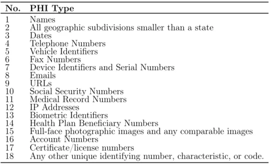
There are two separate pathways for de-identifying data according to HIPAA: Expert Deter-mination, where an expert determines if the information is no longer individually identifiable, and Safe Harbor, which requires all 18 personal identifiers to be removed, as specified in Ta-ble 1.1 [11]. Since the project studied automated de-identification systems, we focused on Safe Harbor method.

No. PHI Type

1 Names

2 All geographic subdivisions smaller than a state

3 Dates

4 Telephone Numbers 5 Vehicle Identifiers 6 Fax Numbers

7 Device Identifiers and Serial Numbers

8 Emails

9 URLs

10 Social Security Numbers 11 Medical Record Numbers 12 IP Addresses

13 Biometric Identifiers

14 Health Plan Beneficiary Numbers

15 Full-face photographic images and any comparable images 16 Account Numbers

17 Certificate/license numbers

18 Any other unique identifying number, characteristic, or code. Table 1.1: Personal identifiers defined by HIPAA Safe Harbor legislation.

1.3 De-identification as Named Entity Recognition

Most healthcare data are stored in unstructured free-text notes as part of a patient’s EHR. Hence, it is difficult to de-identify personal information as it includes abbreviations,

(19)

mis-spellings, and ungrammatical sentences. Manual de-identification also requires an extensive amount of time and cost. For instance, human de-identification of 2,785 nursing progress notes in the MIMIC-II database with 356,103 words costs $3,200 for 56 hours [6]. Extrapolat-ing this to the MIMIC-III database, which consists of 223,556 nursExtrapolat-ing notes with an average 358 words per note, would mean that de-identifying MIMIC-III would require $720,794 and 12,585 hours! Thus, a need for automated de-identification systems exists.

De-identification can be seen as a Named Entity Recognition (NER) problem that aims to label words in a given text into pre-defined categories such as names and locations. NER is defined as a two-step process: 1. detect a named entity, and 2. categorize the entity. Traditional approaches to NER involve dictionaries and gazetteers of person names and locations. However, abbreviations, misspellings, and out-of-vocabulary PHI introduce diffi-culty to these approaches. Many recent challenges emphasize incorporating context in an automated de-identification system.

1.3.1 Recent Challenges

In recent years, there have been many efforts to address the de-identification of electronic health records. The National NLP Clinical Challenges (n2c2) in both 2006 and 2014, formerly known as i2b2 Challenges, featured de-identification tracks focused on identifying PHI in the clinical narratives. The challenge addressed a broader set of PHI entities covered by HIPAA. It had additional categories such as professions, full dates, and other information related to medical workers and facilities. In 2016, the CEGS N-GRID Challenge featured another de-identification track on a new dataset of approximately 1000 initial psychiatric evaluation records. Currently, the CEGS N-GRID dataset is not publicly accessible; only the i2b2 datasets are available with permission. Thus, this research will be evaluated on i2b2 data for model performance comparison.

(20)

(21)

Chapter 2 Related Work

Automated text de-identification traditionally uses two types of methodologies, rule-based and machine learning (ML). Sometimes both methods are combined to target specific PHI types. With recent advances in deep learning models, artificial neural networks (ANN) have become prevalent in recognizing PHI terms.

2.1 Rule-based Methods

Rule-based systems use dictionaries and regular expressions to detect targeted entities [22, 8, 7]. These domain-specific patterns and rules are typically created manually by experts over a long period. The advantage of these methods is that they do not require any labeled data for training and are easy to implement and improve. On the other hand, these methods require complex and unique algorithms for different datasets. Therefore, they are not robust to language changes such as abbreviations. They also have a hard time dealing with ambiguity like "Parkinson’s disease" vs. "Mrs. Parkinson’s" where the former is non-PHI, and the latter is PHI.

2.1.1 LCP method: deid

Our lab, Laboratory for Computational Physiology, developed a simple Perl automated de-identification algorithm for clinical notes, called deid [16]. The software uses pattern

(22)

matching to identify numerical PHI instances, such as dates, telephone numbers, social security numbers, and other protected types of identification numbers. It also uses look-up tables with context checks to identify non-numerical PHI instances, such as locations, patient names, and hospital names. Particularly, the algorithm uses known patient and doctor names from the hospital in the look-up table. This approach is essential to get good performance. Most external applications of this algorithm do not customize it in this way, so they often perform poorly.

Once the algorithm identifies all PHI entities, it replaces each PHI with a corresponding category tag. For example, a NAME entity will be replaced by a masked tag such as [First Name]. For entities in the DATE category, tags can be any randomly generated fake dates. The algorithm is tuned to de-identify PHI in nursing notes and discharge summaries in the MIMIC-II. It can also be customized to handle text files of any format.

2.2 Machine Learning Methods

Recent applications use machine learning algorithms to de-identify clinical notes by training a statistical model that classifies words into a PHI or a non-PHI group. The model further classifies words in the PHI group by their HIPAA categories. Different statistical models include support vector machines (SVM), conditional random field (CRF), and decision tree [9, 2, 30]. Most state-of-the-art systems use CRF because of its high performance in NER tasks. The main advantage of the ML methods is their ability to learn complex patterns in new datasets automatically. However, because these models are supervised learning algo-rithms, they require a large amount of annotated data, which takes an extensive amount of work by experts.

2.3 Combined Methods

Knowing both the advantages and disadvantages of rule-based and ML methods, experts from the field proposed a hybrid model. This model uses pattern matchings to extract features for classification. The extracted features, usually in word-level, are the inputs to

(23)

the ML models [35]. This hybrid method gives an impressive performance, but the feature engineering process could take a long time and is not generalizable to a different dataset.

2.4 Deep Learning Methods

Deep Learning algorithms present a new framework that overcomes drawbacks in earlier methods. These models take vector representations for the inputs (i.e., word embedding) and use multiple ANN layers to learn the relevant features automatically.

Several techniques have been proposed in the field, mainly using recurrent neural networks (RNNs) and Long Short-Term Memory networks (LSTMs) [4, 34]. Traditional RNN uses a loop to allow information to persist. It can be thought of as multiple copies of the same network, with each network passing a message to a successor. This chain-like nature of RNN leads to short-term memory issues - the longer the chain is, the more probable that the information is lost along the chain [19]. LSTM overcomes the short-term memory problems by using special units that selectively remember or forget information. Therefore it enables better preservation of long-range dependencies [12]. However, both RNN and LSTM suffer from the problem of uni-directionality. These models only preserve the information from the inputs that have already been passed through the models. This unidirectionality can hinder the model’s ability to learn the exact meaning of a word since the model cannot incorporate later parts of a sentence into context. Several papers introduced Bi-directional Long Short-Term Memory Network (Bi-LSTM) to solve this unidirectionality problem [21]. Bi-LSTM takes the inputs and runs LSTM in two ways - forward from left to right and backward from right to left. The model then concatenates the two results. However, such representations cannot take advantage of both the left and right context simultaneously [15].

2.4.1 BERT

Many promising modifications have been made to the earlier deep learning methods to im-prove performance. For example, an attention network was proposed to replace recurrent components to capture the relationship between words better [32]. Large scale pretrain-ing of language models has demonstrated a significant improvement in downstream tasks

(24)

[26]. Devlin et al. presented a pre-trained language model named BERT, which achieved state-of-the-art performance on most NLP tasks, including NER [5]. BERT uses a masked language model with transformers that allow pre-trained deep bidirectional representations for a sequence. It combines two key ideas to overcome the limitations in the earlier models: transformer architecture and transfer learning.

Transformer Architecture

BERT is formulated on transformer architecture by applying a self-attention mechanism. The attention mechanism allows the model to look at the entire sentence and selectively extract the information it needs when interpreting a word [32]. This mechanism resembles human reading attention. When reading a text, humans always focus on the word we read. At the same time, our mind still remembers the important keywords to provide context. The attention mechanism enables long-range dependencies and parallelization since it ultimately considers every word when interpreting a word.

Transfer Learning

Transfer learning is a process of training a model on a large-scale dataset and then using that pre-trained model for a downstream task. Recent work suggests that using a pre-trained language model can significantly improve NER tasks’ performance and reduce the burden of a large labeled dataset for supervised learning [13]. One example is Embedding from Language Models (ELMo), which uses Bi-LSTMs trained on a language modeling objective and beats previous performance benchmarks [25].

Combining the above two ideas, BERT outperformed earlier NLP models. The research, therefore, focused on using a pre-trained BERT to de-identify patient notes.

2.5 State-of-the-art Models

Current best performing models for de-identification include PHILter algorithm, Dernon-court et al. model, and Liu et al. model. While PHILTer is built on rule-based and

(25)

statistical models, the other two models are built on RNN architectures. Table 2.1 reports binary token performance (defined in Section 4.6) of these three models.

Model Recall Precision F1

PHILter 99.92 78.58 94.77

Dernoncourt et al. 97.83 97.92 97.88 Liu et al. 97.28 99.30 98.28

Table 2.1: Binary token performance of current state-of-the-art models trained on the i2b2 2014 training dataset and evaluated on the i2b2 2014 test dataset.

2.5.1 PHILter

Protected Health Information Filter, known as PHILter, is a customizable open-source de-identification software. The algorithm uses an overlapping pipeline of multiple state-of-the-art methods, including pattern matching, statistical modeling, blocklist, and allowlist, to remove PHI from free-text clinical notes [23]. The software achieved the highest reported recall score on the i2b2 2014 test corpora.

2.5.2 Dernoncourt et al.

Dernoncourt et al. model, detailed in [4], was the first de-identification system based on recurrent neural networks. The system is composed of three layers: 1. character-enhanced token embedding layer, 2. label prediction layer, and 3. label sequence optimization layer. It demonstrated that combining RNNs with CRFs and training the model from end-to-end can achieve a promising performance.

2.5.3 Liu et al.

Liu et al. model, detailed in [21], extended Dernoncourt et al. model by adding additional context features to the neural network. Liu et al. proposed a hybrid method that used an ensemble classifier to combine different methods: a CRF-based method, a bidirectional LSTM with hand-crafted features, a regular bidirectional LSTM, and a rule-based method. The system achieved a state-of-the-art F1 score of 98.28%.

(26)

(27)

Chapter 3 Dataset

Four datasets were used in this research, i2b2 2006, i2b2 2014, Physionet, and Dernoncourt-Lee. This research focused on i2b2 2014 dataset since it is publicly available, and several recent papers use it for evaluation.

3.1 i2b2

3.1.1 i2b2 2006

This database was used in the i2b2 challenge in 2006. It consists of 889 discharge summaries, one record per patient, with 19,498 PHI instances drawn from Partners Healthcare System, a Boston-based hospital network. All authentic PHI are replaced with synthesized surrogates. The i2b2 2006 challenge aimed to focus on non-dictionary-based de-identification methods, so this database was enriched with out-of-vocabulary PHI surrogates, i.e., made-up names. It includes doctor and hospital names in addition to the categories defined by HIPAA [31].

3.1.2 i2b2 2014

This database was used in the i2b2 challenge in 2014. It consists of a newly de-identified corpus of longitudinal medical records, drawn from Partners Healthcare System. The 2014 challenge paid particular attention to longitudinal clinical narratives, which claimed to con-tain more PHI instances than individual records used in the 2006 challenge. "This

(28)

infor-mation, while perfectly HIPAA-compliant and ineffective for identifying the patient when found in individual records and on their own, can be used collectively to piece together the identity of the patient over several records" [29].

The dataset consists of 1,304 medical records with 28,867 PHI instances for 296 diabetic patients. It uses additional categories for PHI and defines a stricter standard than the rules defined by HIPAA (e.g., It has categories such as professions, full dates, and information related to medical workers and facilities). All instances of PHI in these records have been removed and replaced with realistic surrogates.

3.2 PhysioNet

PhysioNet dataset consists of 2,434 nursing notes collected from patients admitted to ICU at Beth Israel Deaconess Medical Center (BIDMC) in Boston [22]. The nursing progress notes are unstructured free text typed by nurses daily. The notes include observations about the patient’s current physical state, medical history, medications administered, and other medical-related information. Compared with other forms of medical notes like discharge summaries, nursing notes are challenging to de-identify because they include more technical terminologies, frequent abbreviations, and incorrect punctuations. Similar to i2b2 data, PhysioNet data was fully de-identified with all PHI instances replaced with surrogate PHI.

3.3 Dernoncourt-Lee

The Dernoncourt-Lee dataset was used by Dernoncourt et al. in the creation of their de-identification model [4]. The dataset was created as follows. A rule-based de-de-identification system was applied on the MIMIC-III database, consisting of 2 million de-identified patient notes and 1,635 de-identified discharge summaries, each belonging to a different patient admitted to ICU at BIDMC. A total of 60,730 PHI instances were annotated.

(29)

3.4 Dataset Summary

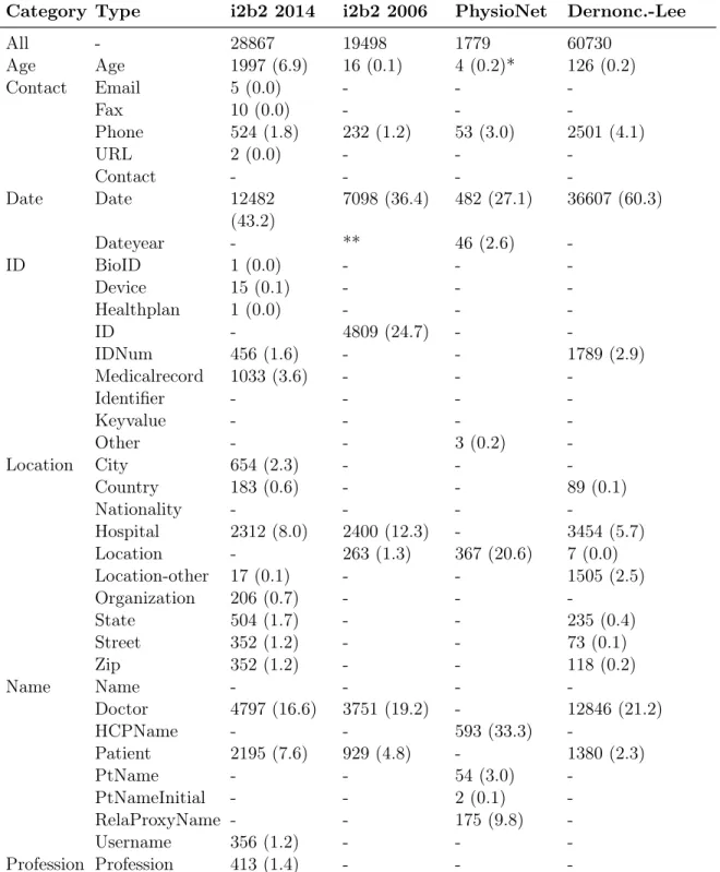
Table 3.1 shows distribution and characteristic of four datasets. This research used all datasets in their entirety. Different datasets use different annotations for certain entity types. The i2b2 2006 dataset adds two entity types to HIPAA categories, DOCTOR and HOSPITAL. YEAR is not PHI in i2b2 2006. It contains out-of-vocabulary and ambiguous surrogate PHI to prevent heavy use of dictionaries. The i2b2 2014 dataset introduces more than two entity types such as PROFESSION, and the types are more varied compared to i2b2 2006. In the PhysioNet dataset, ages under 89 are not PHI. Dernoncourt-Lee has similar annotations as i2b2 2014.

Categories like DATE and NAME have a large number of PHI entities in all datasets. Categories like AGE, CONTACT, and ID have a small number of PHI entities in most datasets. In PhysioNet, there are only a few AGE and ID entities.

Because annotations differ across datasets, we apply harmonization to group different en-tity types into a more general, related category before training. Table 3.1 shows the groupings of different annotations. For example, category CONTACT includes entity types like email, fax number, phone number, URL, and contacts. Categories ID includes any ID-related entity types like BioID, Device ID, and medical record number. Category LOCATION includes entity types like city, country, nationality, and hospital.

(30)

Category Type i2b2 2014 i2b2 2006 PhysioNet Dernonc.-Lee All - 28867 19498 1779 60730 Age Age 1997 (6.9) 16 (0.1) 4 (0.2)* 126 (0.2) Contact Email 5 (0.0) - - -Fax 10 (0.0) - - -Phone 524 (1.8) 232 (1.2) 53 (3.0) 2501 (4.1) URL 2 (0.0) - - -Contact - - - -Date Date 12482 (43.2) 7098 (36.4) 482 (27.1) 36607 (60.3) Dateyear - ** 46 (2.6) -ID BioID 1 (0.0) - - -Device 15 (0.1) - - -Healthplan 1 (0.0) - - -ID - 4809 (24.7) - -IDNum 456 (1.6) - - 1789 (2.9) Medicalrecord 1033 (3.6) - - -Identifier - - - -Keyvalue - - - -Other - - 3 (0.2) -Location City 654 (2.3) - - -Country 183 (0.6) - - 89 (0.1) Nationality - - - -Hospital 2312 (8.0) 2400 (12.3) - 3454 (5.7) Location - 263 (1.3) 367 (20.6) 7 (0.0) Location-other 17 (0.1) - - 1505 (2.5) Organization 206 (0.7) - - -State 504 (1.7) - - 235 (0.4) Street 352 (1.2) - - 73 (0.1) Zip 352 (1.2) - - 118 (0.2) Name Name - - - -Doctor 4797 (16.6) 3751 (19.2) - 12846 (21.2) HCPName - - 593 (33.3) -Patient 2195 (7.6) 929 (4.8) - 1380 (2.3) PtName - - 54 (3.0) -PtNameInitial - - 2 (0.1) -RelaProxyName - - 175 (9.8) -Username 356 (1.2) - - -Profession -Profession 413 (1.4) - -

-Table 3.1: Categories and type attributes of PHI entities (n, %) in each dataset. *In the PhysioNet corpus, ages under 89 years are not treated as PHI. **In the i2b2 2006 corpus, year is not annotated as PHI.

(31)

Chapter 4 Methods

4.1 Label Processing

4.1.1 Label Harmonization

The harmonization is done by grouping entity types into one of seven entity categories: age, contact, date, location, ID, name, and profession, specified in Table 3.1. An input text is split by space to get each word, which is then labeled with a corresponding category based on its entity type.

4.1.2 Resolve Label Conflict

In some rare cases, a word might have more than one annotation. For instance, "Home/Bangdung" is considered one word when splitting text by space. However, "Home" has an entity type HOSPITAL, "/" has no entity type, and "Bangdung" has an entity type CITY. We resolve these conflicts by further splitting on the conflict label. In this case, the word is further split into three subwords to represent three different entity types: "Home", "/", and "Bangdung".

4.1.3 BIO scheme transformation

We transform the entity tag for each word using the BIO scheme. We use B- prefix before a tag to indicate the tag is the beginning of a PHI entity, an I- prefix before a tag to indicate

(32)

the tag is a continuation of the same entity, and an O tag to indicate all other non-PHI words. Table 4.1 shows an example of final tags for an input text "Patient presented to Massachusetts General Hospital on".

Text Patient presented to Massachusetts General Hospital on

Label O O O B-Loc I-Loc I-Loc O

Table 4.1: Final label for the given input text after label harmonization and BIO scheme transformation

4.2 Pipeline Overview

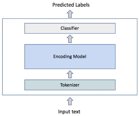
Figure 4-1 shows an illustration of the experimented system pipeline: a tokenizer, an encoding model, and a classifier. Given an input text, the system outputs predicted labels for each word in the input text.

Figure 4-1: Pipeline of the experimented system.

(33)

get a sequence of tokens, which is then fed into an encoding model to output an encoded token sequence. The final hidden states of the encoded token sequence are fed into a classifier for the domain-specific task. This classification model aims to learn and project the encoded token representation into a tag space (i.e., entity categories). Lastly, the model outputs a sequence of predicted labels.

4.2.1 Experimentation

The study experimented with different method combinations to achieve state-of-the-art per-formance. An outline of the methods for each section in the pipeline as follows.

∙ Tokenizer

– WordPiece – ByteLevelBPE

* RoBERTa

* Retrain on domain-specific data

∙ Encoding Model – BERT – BioBERT – ClinicalBERT – RoBERTa – Ensemble Model ∙ Classifer

– Dense layer only

(34)

4.3 Tokenizer

Tokenization is a process of splitting a text into smaller units called tokens, where each token can be either a character, a word, or a subword. These tokens are used to prepare a vocabulary, which commonly consists of all unique tokens or the top K frequently occurring tokens in the corpus.

In NLP, tokenization is the foremost step when processing the raw text data. Tokeniza-tion can be broadly classified into three categories: word, character, and subword. Word tokenization splits a text into individual words based on certain delimiters like space and punctuation. One major issue of word tokenization is Out of Vocabulary (OOV) words, which refer to the new words that do not exist in the vocabulary. Character tokenization splits a text into a set of characters. It handles OOV words by breaking them down into known characters. However, character tokens limit the model’s ability to learn meaningful representations of the text, since lengths of the inputs and the outputs increase rapidly in character level. Lastly, subword tokenization is a hybrid between word and character tok-enization. Subword tokenization splits a text into subwords or n-gram characters. The main idea is that most common words should be left as is, but rare words should be decomposed in meaningful subword units. For instance, rare words like lowest can be broken into low and est.

One of the widely used subword tokenization is Byte-Pair Encoding (BPE). BPE iter-atively merges the most frequently occurring characters until the algorithm has learned a vocabulary of the desired size. BPE addresses OOV words effectively by representing them in terms of known subwords. It also gives a meaningful representation of words as lengths of inputs and outputs are much shorter compared to character tokens. In this study, two types of subword tokenization experimented: WordPiece and Byte Level BPE. Both are alternative forms of Byte-Pair Encoding with minor differences.

4.3.1 WordPiece

BERT uses WordPiece tokenization when pretraining [28]. WordPiece works similarly to BPE, where vocabulary initially starts with every character in the corpus and progressively

(35)

merges characters. The only difference is that the merge rule relies on maximizing the likelihood of the training data instead of merging the most frequent pair. In our experiment, all encoding models used WordPiece as the tokenizer except RoBERTa.

4.3.2 Byte Level Byte-Pair Encoding

Byte Level BPE is the tokenization algorithm used for RoBERTa [27]. It relies on a space pre-tokenizer that splits the training data into words. Byte Level BPE uses bytes as the base vocabulary, and it solves the issue of potential OOV characters in the traditional BPE tokenizer that uses Unicode (e.g., special character emoji). Using bytes limits vocabulary size to 256 with additional rules with punctuation. In this way, Byte Level BPE can represent all possible characters. Byte Level BPE tokenizer used for RoBERTa employs different training schemes by assuming words are separated by a single space. The input text was preprocessed by replacing all new line and tab characters with space and later removing additional space between the words.

4.3.3 Retrain Byte Level BPE on Biomedical Corpus

Both WordPiece and Byte Level BPE were pretrained to work well on general English cor-pora. However, it is not a trivial task for languages in the biomedical domain because of specific terminologies. For instance, pneumothorax is a common word in a radiology report, but it rarely appears in general English text. The tokenizers trained on the general cor-pus would break down the word into many prefix and suffix, instead of leaving it as one word. Therefore, this experiment also used a byte-level BPE tokenizer that retrained on biomedical contents. Once the tokenizer picks up those frequent biomedical-related words, the RoBERTa model is retrained with this new tokenizer [10].

4.3.4 Data Generation

A tokenizer takes an arbitrary span of contiguous text up to 𝑁 tokens. It does not restrict the input sequence to only a linguistic sentence. This, in turn, gives the advantage of incorporating document context instead of sentence context.

(36)

We break up each medical record into overlapping spans of length up to 𝑁 and use a stride of 𝑆 tokens to avoid loss of information flow. Figure 4-2 shows an example with 𝑁 = 6 and 𝑆 = 1. Each span is used as an individual input sequence when training a tokenizer. In our experiment, 𝑁 equals the maximum sequence length that BERT and RoBERTa allow, which are both 512, and 𝑆 equals 10% of 𝑁 . When different predictions occur for a token repeated in multiple spans, a finalized label is chosen based on the highest valued prediction. i.e., The tag with the highest probability becomes the final predicted label. When there is a tie, the first one will be the final label.

Figure 4-2: An example of tokens generated with an input token sequence that has a size of 11. Larger than N = 6 token sequence is broken into multiple spans with a stride of S = 1.

4.4 Encoding Model

The pretrained language networks used in the encoding model are adopted from Huggingface library v2.10.0 [33]. We finetuned the entire system from end to end, including the weights in the pretrained encoding model. All encoding models used Adam optimizer with a learning rate of 5e-5 and a linear warmup and decay. Models were trained for three epochs with a batch size of 8 on a single NVIDIA Quadro GV100 using CUDA 10.1 and PyTorch v1.4.0. [24].

4.4.1 BERT

BERT is a pretrained transformer encoder stack that consists of 𝐿 identical transformer blocks [32]. Two sizes of BERT were adopted, base and large. Both were trained on BooksCorpus and English Wikipedia, which contains 800M and 2,500M words, respectively. The base version has 12 layers of transformer blocks, 12 attention heads, and 768 hidden

(37)

units, leading to a total of 110M parameters. The large version has 24 layers, 16 heads, and 1,024 hidden units, leading to a total of 340M parameters. Both versions have cased and uncased tokens.

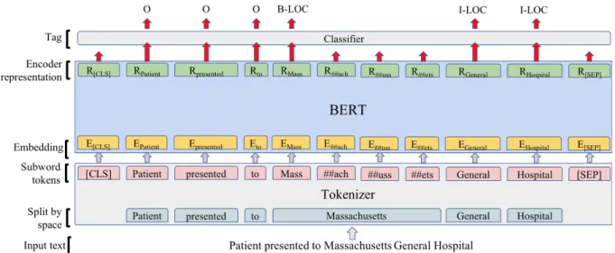
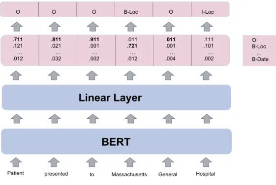
Figure 4-3 shows a pictorial representation of the system with WordPiece tokenizer, BERT as the encoding model, and a linear classifier. The input text "Patient presented to Massachusetts General Hospital" is tokenized and fed into BERT with initial pretrained weights. BERT outputs 𝐿 layers of hidden weights, and the weights from the last layer are fed into a linear classifier to get a predicted tag for each token.

Figure 4-3: The architecture of a system with WordPiece tokenizer, BERT as the encoding model, and a linear classifier.

4.4.2 Domain-specific BERT

BERT is pretrained and tested on general domain text where the word distribution can be quite different from the biomedical text. It can be challenging to estimate the model’s performance on our clinical datasets. For instance, Parkinson’s disease, a non-PHI term, might be identified as a name PHI instance by BERT. Thus, domain-specific BERT models were also evaluated in the experiment, namely BioBERT and ClinicalBERT.

(38)

BioBERT

BioBERT has the same structure as the BERT base-cased model. It trained additionally on biomedical corpora such as PubMed abstracts and PMC full-text articles, which contain approximately 4.5B words and 13.5B words respectively. BioBERT has shown promising performance on biomedical related corpora. Specifically, it achieves a higher F1 score in biomedical NER [18]. With minimal modification, we adopted BioBERT-BASE v1.1 to address biomedical content in our data.

ClinicalBERT

ClinicalBERT is an application of the BERT model to clinical text. It used BioBERT-Base v1.0 and pretrained additionally on clinical notes from MIMIC-III [14]. Two models of ClinicalBERT were used, one was pretrained only on de-identified discharge summaries, and the other was pretrained on all notes from MIMIC-III. Note the PHI tokens in the de-identified notes are replaced with masked tags that correspond to their categories. For instance, a name PHI is replaced with [** name **].

4.4.3 RoBERTa

RoBERTa has the same architecture as BERT but uses a byte-level BPE as the tokenizer and is pretrained on a new English corpus totaling over 160GB of uncompressed text [20]. It also modifies key hyperparameters and training strategies (e.g., trained longer with bigger batches over more data). RoBERTa has demonstrated better downstream task performance. It has two model sizes where the base version has 125M parameters, and the large version has 355M parameters. Unlike BERT, which has both cased and uncased versions, RoBERTa uses bytes to build up its tokenizer’s vocabulary. Thus, it cares about the case sensitivity of a character.

4.4.4 Ensemble Model

Since some categories of PHI instances are very formulaic and rarely occur in the overall dataset, rule-based methods would help identify and extract these features from the raw

(39)

text. Examples include numerical PHI, such as telephone number, fax number, and social security number. Other formulaic categories, like email addresses and URLs, are also easily identified using regular expressions. Models that combine ML approaches with rule-based approaches show promising performance in de-identification. Thus, we proposed that an ensemble model of a pretrained language network with additional rules.

Two rule-based software were used in the experiment, Python version of deid and PHILter, detailed in 2.1.1 and 2.5.1 respectively. The software deid can identify thirteen entity types: age, date, email, ID number, name initials, location, medical record number, name, pager, social security number, telephone number, unit, and URL. To better evaluate a change in performance regarding individual entity type, we examined ensemble models with each rule. Since PHILter can only distinctly identify the DATE entities, only entity type DATE was examined for models ensemble with PHILter.

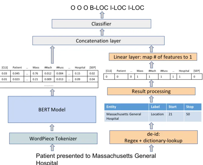
The ensemble system works as follows. Given a text and a target entity type, the rule-based algorithm outputs the start and the end locations of desired entities. The model uses these locations to create a vector of 0s and 1s compatible with the encoding model’s token representation. 1 indicates if the current token is a PHI detected by the rule-based algorithm and 0 otherwise. The vector is fed into a linear layer to get a vector representation of the rule-based results. The output vector is then concatenated with the encoding model’s final hidden layer representation before fed into a classifier. Figure 4.4.4 shows a pictorial architecture of the system with WordPiece tokenizer, a BERT ensemble with deid rule as the encoding model, and a linear classifier.

4.5 Classifier

The classifier takes the last hidden layers from the encoding model and maps the hidden weights into a tag space. We examined two classifiers: a single dense layer, and a CRF on top of a dense layer.

(40)

Figure 4-4: Architecture overview of a system with WordPiece tokenizer, an ensemble model of BERT and deid, and a linear classifier. On the left, WordPiece tokenizes the text and passes tokens into a BERT, which outputs encoded token representations. On the right, deid outputs each entity locations. The model uses these locations to create a vector of 0s and 1s to indicate which tokens are PHI instances identified by deid. For the given example, deid detects "Massachusetts General Hospital". The vector, thus, has 1s on all the tokens describing these PHI words, and 0 otherwise. This vector is fed into a linear layer and then concatenated with BERT outputs before feeding into the classifier.

4.5.1 Linear Only

The linear classifier predicts a tag sequence that minimizes the cross-entropy loss. It predicts labels one at a time by taking the maximum over the current token probability distribution. Figure 4.5.1 shows a linear classifier predicts a label by softmax the probability distribution locally.

(41)

Figure 4-5: Tag prediction using a single linear layer as the classifier.

4.5.2 Linear with CRF

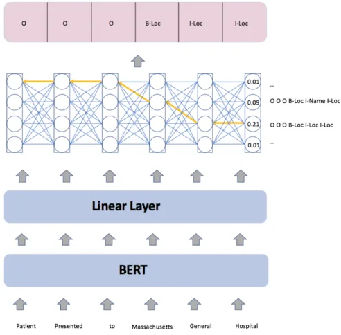
The second classifier is adding a CRF layer on top of a linear layer. CRF is a statistical model that maximizes the log-probability of the entire tag sequence in the last token. It aims to learn relationships between entity types. CRF can help ensure a tag transition from B-location to I-Date would never happen since such transition has a very low probability. Figure 4-6 shows a prediction made by a CRF classifier. CRF predicts the entire tag sequence at the last token by looking at which labeling gives the maximum overall probability.

4.5.3 Loss Aggregation for Subword tokens

BERT uses the first subword token representation as the input to the NER classifier. For in-stance, WordPiece tokenizes Massachusetts into four subword tokens: Mass, ##ach, ##uss, and ##ets. The word Massachusetts has label B-Location for all of its subword tokens. This labeling choice does not change the BERT model’s behavior and performance. When calculating the loss and evaluating the model performance, B-Location labels introduced on the additional subword tokens are ignored. In this way, additional B-Location labels

(42)

Figure 4-6: Tag prediction using a linear layer with a CRF layer for the classifier.

would not affect the support number of B-Location class.

4.6 Evaluation Measures

The evaluation measures used are precision, recall, and F1-score. Precision measures the ability of a NER model to identify only correct named entities; recall measures the ability to identify all named entities; F1-score is the harmonic mean of precision and recall. The micro-averaged F1 score is our primary measure.

There are two levels of evaluation: entity and token. Entity level requires outputs to match exactly the beginning and the end locations of each PHI tag, a standard evaluation system for the NER problem. Token level evaluation can be on a per-token basis without matching the exact location. For example, "Rayna De Angelis" has a gold annotation of

(43)

NAME, token-based evaluation allows "Rayna", "De", and "Angelis" to have individual tags. In contrast, entity-based evaluation needs "Rayna De Angelis" to be captured as a whole tag. In terms of de-identification, we only care that all parts of a single PHI are identified at some point. Whether they are identified together as one phrase or separably is not a concern. Thus, we favor token evaluation over entity evaluation in this study.

Since the final goal of de-identification is to remove PHI, the focus is to identify all PHI with less emphasis on correct entity type predictions. Thus, we care more about binary performance where we group labels into either PHI or not PHI when evaluating.

4.6.1 Tokenization Scheme

Different tokenizers pre-tokenize text differently to get initial tokens. WordPiece splits on space and all punctuations. Byte Pair BPE splits on space only. PHILter uses nltk tokenizer, which splits on space and certain punctuations (e.g., Commas and periods are separate to-kens. Quotes are kept.) [23, 3]. The variances in the splitting delimiters lead to a different form of the tokens. Thus, the evaluation uses three tokenization schemes: space only, space with all punctuations, and nltk. Different tokenization scheme would only affect token eval-uation but not entity evaleval-uation.

WordPiece and Byte Level BPE further tokenize rare words into subwords. We flag the entire token as PHI if any of its subwords is flagged during evaluation. For example, the word "Rayna" is split into "Ray" and "na" by WordPiece. If a model predicts "Ray" as PHI and "na" as non-PHI, the entire token "Rayna" will be treated as PHI during evaluation.

4.6.2 Relaxed Evaluation: Ignore Missed Punctuations

Our dataset contains inconsistent labeling with punctuation. In some cases, parentheses around a phone number are included in a PHI instance; in other cases, they are not. Occa-sionally PHI instances ended with punctuation have the punctuation as PHI. Due to different tokenization schemes, we allow a relaxed token evaluation. The misclassified punctuation at the beginning and the end of a token is ignored during the evaluation.

(44)

(45)

Chapter 5 Results

We present the results as follow: (1) the impact of tokenization scheme on token evaluation, (2) the impact of encoding model with design choices such as size, case sensitivity, and pretrained weights, (3) the impact of the classifier, and (5) the impact of the rules used in ensemble models. We focus on i2b2 2014 dataset for most model performance comparisons. We further assess the generalizability of the model using the remaining datasets.

5.1 Effect of Tokenization Splitting Scheme on Token

Eval-uation

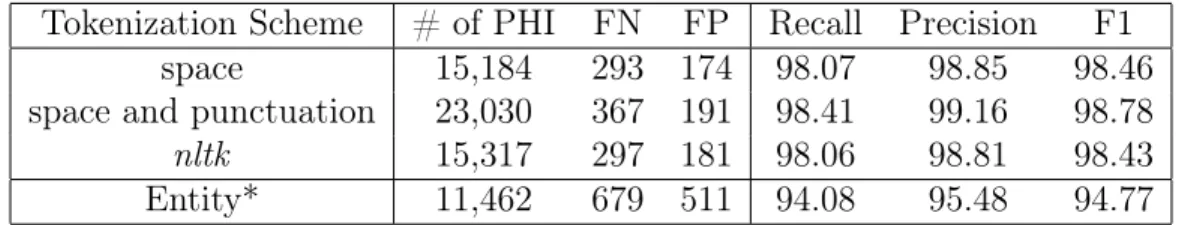
Tokenization strategies affect model performance during token evaluation. Table 5.1 shows BERT base-uncased performance using three tokenization schemes. BERT uses WordPiece to tokenize text by space and punctuation, which explains a slight improvement in the token evaluation using space and punctuation splitting scheme. However, it is hard to conclude if the improvement comes from the better splitting strategy since punctuation delimiter introduces twice as much PHI tokens as space delimiter does. Additional PHI tokens mainly come from DATE entities, consisting of 40% of the i2b2 2014 dataset. The punctuation delimiter splits these DATE entities into two or more tokens (e.g., 08/20/2005 would be tokenized into three tokens 08, 20, and 2005). Therefore, punctuation delimiter adds more weight to true positive score if a space delimiter alone can identify most DATE entities.

(46)

Tokenization Scheme # of PHI FN FP Recall Precision F1

space 15,184 293 174 98.07 98.85 98.46

space and punctuation 23,030 367 191 98.41 99.16 98.78

nltk 15,317 297 181 98.06 98.81 98.43

Entity* 11,462 679 511 94.08 95.48 94.77

Table 5.1: Binary token performance of BERT𝑏𝑎𝑠𝑒,𝑢𝑛𝑐𝑎𝑠𝑒𝑑 with a linear classifier trained on

i2b2 2014 and evaluated with different tokenization splitting scheme. Relaxed* binary entity performance is the same for all tokenization schemes.

Table 5.2 shows that space delimiter gives the best token evaluation for RoBERTa, which uses Byte Level BPE to tokenize text by space. There are many numerical false negative entities, including Date entities. Further splitting of these Date entities by punctuation leads to an increase in the number of false negatives, which explains the lower performance using space and punctuation delimiter.

The i2b2 challenge used space delimiter to define a token. To be consistent with past de-identification evaluation methods, the rest of this paper will report performance using a space delimiter.

Tokenization Scheme # of PHI FN FP Recall Precision F1

space 15,184 940 143 93.81 99.01 96.34

space and punctuation 23,030 1,808 649 92.15 97.03 94.53

nltk 15,317 941 220 93.86 98.49 96.12

Entity* 11,462 4,344 3,341 62.10 68.06 64.94

Table 5.2: Binary token performance of RoBERTa𝑏𝑎𝑠𝑒 with a linear classifier trained on i2b2

2014 and evaluated with different tokenization splitting scheme. Relaxed* binary entity performance is the same for all tokenization schemes.

5.2 BERT as the Encoding Model

5.2.1 Effect of Size and Case Sensitivity

Table 5.3 shows the confusion matrix of BERT base-uncased trained with a linear classifier. Table 5.4 shows binary and multi-token performances of different versions of BERT mod-els. Sensitivity (Se, also known as recall), positive predictive value (PPV, also known as precision), and F1 scores are reported. Large models outperform corresponding base models

(47)

by an average of 0.3%. This increase is not appreciatively better compared to millions of parameters learned in large models. In both base and large models, case-insensitive versions outperform the case-sensitive version. Thus, uncased models are favorable when constructing ensemble models.

Predicted Yes Predicted No

Actual Yes 14,891 293

Actual No 174 316,038

Table 5.3: Confusion matrix for BERT𝑏𝑎𝑠𝑒,𝑢𝑛𝑐𝑎𝑠𝑒𝑑 along with a linear classifier trained and

evaluated on the i2b2 2014 dataset.

The multi-token performance drops 0.4 - 0.6% across models. The errors mainly come from incorrect predictions among similar categories like NAME and LOCATION. For in-stance, "Una Trujillo" is predicted as LOCATION instead of its true annotation, NAME. "Olney" is predicted as NAME instead of LOCATION.

Model Binary Multi

Se PPV F1 Se PPV F1

BERT𝑏𝑎𝑠𝑒,𝑢𝑛𝑐𝑎𝑠𝑒𝑑 98.07 98.85 98.46 97.58 98.49 98.03

BERT𝑏𝑎𝑠𝑒,𝑐𝑎𝑠𝑒𝑑 97.54 98.81 98.17 96.96 98.35 97.65

BERT𝑙𝑎𝑟𝑔𝑒,𝑢𝑛𝑐𝑎𝑠𝑒𝑑 98.47 99.10 98.78 98.03 98.77 98.40

BERT𝑙𝑎𝑟𝑔𝑒,𝑐𝑎𝑠𝑒𝑑 97.98 99.12 98.55 97.42 98.71 98.06

Table 5.4: Binary and multi-token performance of a BERT model with different sizes and case sensitivity along with a linear classifier trained and evaluated on the i2b2 2014.

5.2.2 Effect of Pretrained Weights

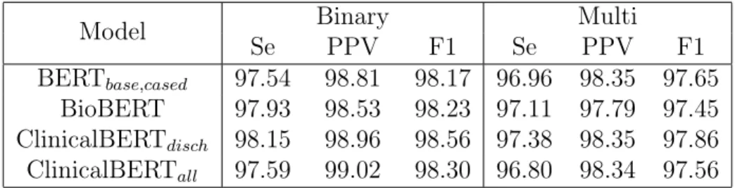
Table 5.5 shows BERT performances using different pretrained weights. Pretrained weights from additional biomedical or clinical related corpus improve performance in binary evalu-ation but decrease performance in multi-class evaluevalu-ation for some models (e.g., BioBERT and ClinicalBERT trained on all notes).

ClinicalBERT that trained only on discharge summaries gives the optimal performance. This result differs from [1] paper, where the authors claimed that pretrained weights on clinical data are not performant on identification tasks. The authors argued that de-identification datasets have different text distribution from MIMIC-III, a database used for

(48)

pretraining ClinicalBERT. The i2b2 datasets use synthetically-masked PHI, but MIMIC data use sentinel PHI symbols at locations where PHI was removed. One explanation of the difference in results might be the case-sensitivity of the model. It is not clear which BERT model the authors used for reference in their comparison. The results from Table 5.4 demonstrate that case sensitivity plays a significant role in model performances, and both BioBERT and ClinicalBERT were based on the cased version of BERT.

Interestingly, ClinicalBERT trained only on discharge summaries gives better perfor-mance than the one trained on all notes. It suggests that adding higher specificity to the underlying corpus can be helpful for our de-identification task.

Model Binary Multi

Se PPV F1 Se PPV F1

BERT𝑏𝑎𝑠𝑒,𝑐𝑎𝑠𝑒𝑑 97.54 98.81 98.17 96.96 98.35 97.65

BioBERT 97.93 98.53 98.23 97.11 97.79 97.45 ClinicalBERT𝑑𝑖𝑠𝑐ℎ 98.15 98.96 98.56 97.38 98.35 97.86

ClinicalBERT𝑎𝑙𝑙 97.59 99.02 98.30 96.80 98.34 97.56

Table 5.5: Binary and multi-token performance of a BERT model with different pretrained weights along with a linear classifier trained and evaluated on the i2b2 2014.

5.3 Effect of Encoding Model

5.3.1 BERT vs RoBERTa

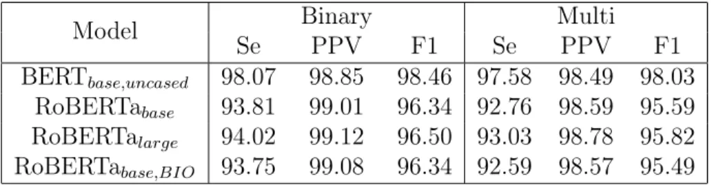
Table 5.6 shows performances with a BERT or a RoBERTa as an encoding model. RoBERTa retrained on biomedical corpus has no impact on the performance. Surprisingly, both base and large RoBERTa perform noticeably worse than the BERT base model. This result is different from [20] paper, which shows that RoBERTa gives a state-of-the-art performance in most downstream tasks. In our case, RoBERTa has difficulty in recognizing numerical entities such as DATE, ID, and CONTACT, shown in Tables A.1 and A.2.

Looking at individual errors in Table 5.7, many false negative PHI entities are preceded by non-space characters, which are usually not parts of PHI instances. RoBERTa defines a non-first subword token as any token that is not preceded by a space. The model aggregates the loss to the first subword token when training. Therefore, RoBERTa would treat the

(49)

Model Binary Multi Se PPV F1 Se PPV F1 BERT𝑏𝑎𝑠𝑒,𝑢𝑛𝑐𝑎𝑠𝑒𝑑 98.07 98.85 98.46 97.58 98.49 98.03 RoBERTa𝑏𝑎𝑠𝑒 93.81 99.01 96.34 92.76 98.59 95.59 RoBERTa𝑙𝑎𝑟𝑔𝑒 94.02 99.12 96.50 93.03 98.78 95.82 RoBERTa𝑏𝑎𝑠𝑒,𝐵𝐼𝑂 93.75 99.08 96.34 92.59 98.57 95.49

Table 5.6: Binary and multi-token performance of a BERT and a RoBERTa model with a linear classifier trained and evaluated on the i2b2 2014.

entire token as non-PHI if the first subword token is non-PHI, despite the later part is PHI. This issue can explain degradation in performance when using the RoBERTa model.

PHI Category Examples of false negative PHI instances

Date D:07/20/83

KYLE∧02/14/90∧ CHANEY ID eScription document:1-1277442

EDVISIT∧56040785∧OROZCO

Name DVISIT∧56040785∧OROZCO,

Table 5.7: Examples of the false negatives (shown in bold) cannot be identified by the RoBERTa𝑏𝑎𝑠𝑒 but can be identified by BERT𝑏𝑎𝑠𝑒,𝑢𝑛𝑐𝑎𝑠𝑒𝑑. Note that the tokenizer would not

split on the character ∧ by default.

5.3.2 Ensemble Model

Table A.4 shows binary token performances of each PHI category using deid and PHILter algorithm. The deid algorithm does a poor job of identifying PHI instances in categories such as contact, ID, and location.

Table 5.8 shows the impact of incorporating Date rules to the BERT large-uncased model. Ensemble models with either rule-based algorithms have no impact or negative impact on the date PHI instances. The ensemble model with both algorithms improves false negatives in a trade-off with false positives. The binary token performance is similar to BERT’s in the date category and higher in all categories. It suggests that incorporating date rule might help detect other PHI categories.

To explore the impact of incorporating rules on both target and non-target PHI cate-gories, Table A.6 shows the performance of the BERT large uncased model ensemble with

(50)

Model Category Date All Binary FN FP Se PPV F1 Se PPV F1 BERT𝑙𝑎𝑟𝑔𝑒,𝑢𝑛𝑐𝑎𝑠𝑒𝑑 57 25 98.96 99.54 99.25 98.47 99.10 98.78 BERT-deid𝑑𝑎𝑡𝑒 57 36 98.96 99.34 99.15 98.20 99.12 98.66 BERT-PHILter𝑑𝑎𝑡𝑒 63 21 98.85 99.61 99.23 98.38 99.15 98.76 BERT-deid -PHILter𝑑𝑎𝑡𝑒 47 36 99.14 99.34 99.24 98.47 99.14 98.81

Table 5.8: Model performance of BERT𝑙𝑎𝑟𝑔𝑒,𝑢𝑛𝑐𝑎𝑠𝑒𝑑 ensemble with rules that only detect Date

instances. The middle column shows the number of false negative (FN) and false positive (FP) along with binary token performance for Category Date. The last column shows binary token performance for all categories.

individual deid rules for each PHI category.

∙ For category Age, incorporating deid does not help false negative. However, specific rules, such as URL, unit number, medical record number, and name, help reduce the number of false positives. Particularly, incorporating URL rule gives the best binary token F1 score for the Age category.

∙ For category Contact, most rules help precision score. The number of false positives drops noticeably with rules such as date, email, medical record number, pager, social security number, and URL. BERT large, uncased model misses only four PHI tokens, which all have rare phone extensions (e.g., x557, 5-8112). The deid algorithm alone cannot identify those four PHI tokens, so incorporating the rules does not help. Adding the URL rule gives the best binary token F1 score for the Contact category.

∙ For category Date, incorporating rules such as initials and social security numbers improves performance. Adding initials rule can catch date abbreviations missed by BERT (e.g., "Mon"). Since a social security number has a similar form as a date, SSN rule also helps identify date PHI instances for binary evaluation.

∙ For category ID, most rules hurt the model performances except idnum and name rules. Incorporating these two rules help the precision score in a small trade-off with the recall. The overall F1 score increases by 0.3% and 0.5%, respectively.

∙ For category Location, additional rules do not help the model performance. Adding location rule degrades the performance as it fails to identify some PHI instances that

(51)

can be identified by BERT. Incorporating the idnum rule achieves the highest binary token F1 score.

∙ For category Name, additional rules hurt model performances. For instance, incorpo-rating initials rule helps the recall score in a significant trade-off with the precision score.

∙ For category Profession, incorporating name and social security number rules help the model performance.

Table 5.9 reports performances of the BERT large, uncased model ensemble with all rules from deid or/and PHILter algorithms. Incorporating all rules hurts the performance. One explanation might be that certain rules, shown in Table A.4, give bad predictions on PHI instances, and therefore adding them can introduce unnecessary or wrong information to the model about potential PHI instances.

Model Binary Multi

Se PPV F1 Se PPV F1 BERT𝑙𝑎𝑟𝑔𝑒,𝑢𝑛𝑐𝑎𝑠𝑒𝑑 98.47 99.10 98.78 98.03 98.77 98.40 deid 87.55 42.25 57.00 72.73 35.29 47.52 PHILter 81.75 74.58 78.00 - - -BERT-deid𝑎𝑙𝑙 98.05 98.98 98.51 97.58 98.61 98.09 BERT-PHILter𝑎𝑙𝑙 98.29 98.95 98.62 97.79 97.18 94.80 BERT-deid -PHILter𝑎𝑙𝑙 98.25 99.15 98.70 97.74 98.75 98.24

Table 5.9: Binary and multi-token performance of BERT𝑙𝑎𝑟𝑔𝑒,𝑢𝑛𝑐𝑎𝑠𝑒𝑑, deid algorithm, PHILter

algorithm, and ensemble models incorporating all the rules using deid and/or PHILter algo-rithms.

5.4 Effect of Classifier

Table 5.10 shows the performances of the BERT model with a single linear classifier or a CRF classifier. The CRF classifier has little improvement in performance. For the large version BERT, the performance even drops.

Table A.3 reports performance on each PHI category with a CRF classifier. CRF classifier improves performance on categories like ID, Location, and Profession because entities in these

(52)

Model Classifier Binary Multi Se PPV F1 Se PPV F1 BERT𝑏𝑎𝑠𝑒,𝑢𝑛𝑐𝑎𝑠𝑒𝑑 Linear Only 98.07 98.85 98.46 97.58 98.49 98.03 Linear with CRF 98.37 98.70 98.54 97.82 98.27 98.04 BERT𝑙𝑎𝑟𝑔𝑒,𝑢𝑛𝑐𝑎𝑠𝑒𝑑 Linear Only 98.47 99.10 98.78 98.03 98.77 98.40 Linear with CRF 98.29 99.07 98.68 97.80 98.72 98.26 Table 5.10: Binary and multi-token performance of the BERT model with a different choice of classifiers.

categories contain a span of multiple tokens. The linear classifier is more likely to predict an invalid tag sequence (i.e., invalid tag transition) for an entity consists of multiple tokens than a single-token entity. CRF can resolve these invalid tag sequences. Other categories like Age usually have entities that only have a single token, so the CRF classifier does not help.

Table 5.11 shows predictions made by a linear classifier versus a CRF classifier. The first three examples show how CRF can fix invalid tag sequences predicted by a linear classifier. In the first example, CRF resolves an invalid tag in the middle where I-Loc follows B-Name. In the second example, I-Profession followed by O is also invalid, CRF can detect the first token to be B-Profession. In the third example, CRF replaces the last token with B-Profession, but the middle word is still predicted as non-PHI. The fourth and fifth examples show some errors that both linear and CRF classifiers can produce. The linear classifier fails to recognize a token immediately precede or after a correctly predicted token, and sometimes it fails to recognize a stand-alone token. For these kinds of errors, CRF cannot do any better.

Category Entity Linear Prediction CRF Prediction

Name Pina CQ/earley B-Name I-Loc B-Name B-Name B-Name B-Name

Profession school administrator O I-Prof B-Prof I-Prof

Profession midwife and director B-Prof O I-Prof B-Prof O B-Prof

Age 18 month B-Age O B-Age O

Name M OSCAR, JOHNNY O B-Name I-Name O B-Name I-Name

Table 5.11: Examples of the predictions made by a linear classifier versus by a CRF classifier, using BERT𝑏𝑎𝑠𝑒,𝑢𝑛𝑐𝑎𝑠𝑒𝑑 model.

(53)

5.5 Cross-dataset Performance

Table 5.12 shows cross dataset performance. We focus only on Name entity since its annota-tion is relatively consistent across datasets. As expected, models consistently degrade when test on datasets other than the one they are trained on. The model trained on the i2b2 2014 dataset generalizes better even though i2b2 dataset has difference source from PhysioNet and Dernoncourt-Lee.

i2b2 2014 i2b2 2006 PhysioNet Dernoncourt-Lee

Se i2b2 2014 98.43 80.35 95.02 88.36 i2b2 2006 91.21 98.96 80.54 86.20 PhysioNet 81.98 35.37 95.02 83.06 Dernoncourt-Lee 92.47 74.07 93.21 98.00 PPV i2b2 2014 99.08 91.07 88.61 94.67 i2b2 2006 95.72 98.80 85.17 96.10 PhysioNet 95.50 92.57 96.33 94.92 Dernoncourt-Lee 88.83 84.29 88.79 97.78 F1 i2b2 2014 98.75 85.37 91.70 91.41 i2b2 2006 93.41 98.88 82.79 90.88 PhysioNet 88.23 51.99 95.67 88.60 Dernoncourt-Lee 90.61 78.85 90.95 97.89

Table 5.12: Cross dataset performance of the Name PHI instances, using the BERT𝑏𝑎𝑠𝑒,𝑢𝑛𝑐𝑎𝑠𝑒𝑑

with a linear classifier. Models are trained using the training dataset specified in the row and evaluated on the test dataset specified in the column.

5.6 Performance Variance

Three models with optimal performance: (1) BERT large uncased, (2) BERT large uncased ensemble with deid initials rule, and (3) BERT large uncased ensemble with date rules from deid and PHILter, are retrained with the same parameters but different seeds for five times. Table 5.13 shows the average and variance of model performances. The BERT model without additional rules is sufficient to identify the same number of PHI instances.

De-identification of free-text clinical notes

De-identification of Free-text Clinical Notes

by

Jing Lin

B.S. Computer Science and Engineering

Massachusetts Institute of Technology, 2019

Submitted to the Department of Electrical Engineering and Computer Science

in partial fulfillment of the requirements for the degree of

Master of Engineering in Electrical Engineering and Computer Science

at the

MASSACHUSETTS INSTITUTE OF TECHNOLOGY

September 2020

c

○ Massachusetts Institute of Technology 2020. All rights reserved.

Author . . . .

Department of Electrical Engineering and Computer Science

August 14, 2020

Certified by . . . .

Dr. Alistair Johnson

Research Scientist

Thesis Supervisor

Accepted by . . . .

Katrina LaCurts

Chair, Master of Engineering Thesis Committee

De-identification of Free-text Clinical Notes

by

Jing Lin

Abstract

Acknowledgments

Contents

List of Figures

List of Tables

Chapter 1

Introduction

1.1

Motivation

1.2

HIPAA Safe Harbor

1.3

De-identification as Named Entity Recognition

1.3.1

Recent Challenges

Chapter 2

Related Work

2.1

Rule-based Methods

2.1.1

LCP method: deid

2.2

Machine Learning Methods

2.3

Combined Methods

2.4

Deep Learning Methods

2.4.1

BERT

2.5

State-of-the-art Models

2.5.1

PHILter

2.5.2

Dernoncourt et al.

2.5.3

Liu et al.

Chapter 3

Dataset

3.1

i2b2

3.1.1

i2b2 2006

3.1.2

i2b2 2014

3.2

PhysioNet

3.3

Dernoncourt-Lee

3.4

Dataset Summary

Chapter 4

Methods