NLTE determination of the calcium abundance and 3D corrections in extremely metal-poor stars

HAL Id: hal-00685158

https://hal.archives-ouvertes.fr/hal-00685158

Preprint submitted on 4 Apr 2012

HAL is a multi-disciplinary open access

archive for the deposit and dissemination of

sci-entific research documents, whether they are

pub-lished or not. The documents may come from

teaching and research institutions in France or

abroad, or from public or private research centers.

L’archive ouverte pluridisciplinaire HAL, est

destinée au dépôt et à la diffusion de documents

scientifiques de niveau recherche, publiés ou non,

émanant des établissements d’enseignement et de

recherche français ou étrangers, des laboratoires

publics ou privés.

corrections in extremely metal-poor stars

Monique Spite, S.M. Andrievsky, F. Spite, Elisabetta Caffau, S. A. Korotin,

Piercarlo Bonifacio, Hans-G. Ludwig, Patrick François, Roger Cayrel

To cite this version:

Monique Spite, S.M. Andrievsky, F. Spite, Elisabetta Caffau, S. A. Korotin, et al.. NLTE

determina-tion of the calcium abundance and 3D correcdetermina-tions in extremely metal-poor stars. 2012. �hal-00685158�

Astronomy & Astrophysicsmanuscript no. aa18773-spite c ESO 2012 April 4, 2012

NLTE determination of the calcium abundance and 3D corrections

in extremely metal-poor stars

⋆ ⋆⋆

M. Spite

_{, S.M. Andrievsky}

_{, F. Spite}

_{, E. Caffau}

_{, S.A. Korotin}

_{, P. Bonifacio}

_{, H.-G. Ludwig}

_{, P. Franc¸ois}

_{, and}

R. Cayrel

1 _{GEPI Observatoire de Paris, CNRS, Universit´e Paris Diderot, F-92195 Meudon Cedex France e-mail : monique.spite@obspm.fr} 2 _{Department of Astronomy and Astronomical Observatory, Odessa National University, T.G. Shevchenko Park, 65014, Odessa, Ukraine, and}

Isaac Newton Institute of Chile, Odessa Branch, Ukraine

3 _{Zentrum f¨ur Astronomie der Universit¨at Heidelberg, Landessternwarte, K¨onigstuhl 12, 69117 Heidelberg, Germany}

ABSTRACT

Context.Calcium is a key element for constraining the models of chemical enrichment of the Galaxy.

Aims.Extremely metal-poor stars contain the fossil records of the chemical composition of the early Galaxy and it is important to compare Ca

abundance with abundances of other light elements, that are supposed to be synthesized in the same stellar evolution phases.

Methods.The NLTE profiles of the calcium lines were computed in a sample of 53 extremely metal-poor stars with a modified version of the program MULTI, which allows a very good description of the radiation field.

Results.With our new model atom we are able to reconcile the abundance of Ca deduced from the Ca I and Ca II lines in Procyon. This abundance is found to be solar.

–We find that [Ca/Fe] = 0.50 ± 0.09 in the early Galaxy, a value slightly higher than the previous LTE estimations.

–The scatter of the ratios [X/Ca] is generally smaller than the scatter of the ratio [X/Mg] where X is a “light metal” (O, Na, Mg, Al, S, and K) with the exception of Al. These scatters cannot be explained by error of measurements, except for oxygen. Surprisingly, the scatter of [X/Fe] is always equal to, or even smaller than, the scatter around the mean value of [X/Ca].

–We note that at low metallicity, the wavelength of the Ca I resonance line is shifted relative to the (weaker) subordinate lines, a signature of the effect of convection.

–The Ca abundance deduced from the Ca I resonance line (422.7 nm) is found to be systematically smaller at very low metallicity, than the abundance deduced from the subordinate lines. Our computations of the effects of convection (3D effects) are not able to explain this difference. A fully consistent 3D NLTE model atmosphere and line formation scheme would be necessary to fully capture the physics of the stellar atmosphere.

Key words. Line : Formation – Line : Profiles – Stars: Abundances – Stars: Supernovae – Galaxy evolution

1. Introduction

An homogeneous sample of 53 metal-poor stars, most of them extremely metal-poor (EMP stars with [Fe/H] < −2.9), has been observed by Cayrel et al. (2004), and Bonifacio et al. (2007, 2009). The aim of this paper is to determine more pre-cisely the calcium abundance in these stars. 120-125 F6.2 — Corr18 NLTE corrections, model (7000,2,-3.5,0.3) These low

Send offprint requests to: M. Spite e-mail: Monique.Spite@obspm.fr

⋆ _{Based on observations obtained with the ESO Very Large}

Telescope at Paranal Observatory, Chile (Large Programme “First Stars”, ID 165.N-0276(A); P.I.: R. Cayrel).

⋆⋆ _{The NLTE corrections of the Ca lines are available in}

elec-tronic form at the CDS via anonymous ftp to cdsarc.u-strasbg.fr (130.79.128.5) or via http://cdsweb.u-strasbg.fr/cgi-bin/qcat?J/A+A/

mass stars have been formed at the very early phases of the Galaxy and the chemical composition of their atmosphere re-flects the yields of the first massive type II supernovae which have a very short life-time. These supernovae produce more “α-elements” (O, Mg, Si, S, Ca) than “iron-peak” elements. In contrast, less massive type I supernovae, which have a much longer life-time and explode later, produce more iron-peak el-ements than α-elel-ements. As a consequence in the atmosphere of the EMP stars formed at the beginning of the Galaxy a rel-ative enhancement of the α-elements (compared to the Sun) is observed. The level of this overabundance is one of the fun-damental parameters of the chemical evolution models of the Galaxy.

On the other hand, the relative production of the α-elements in a supernova depends on the mass of this supernova (e.g. Kobayashi et al., 2006): [Ca/Fe] tends to be lower for more

massive supernovae. Therefore the level of [Ca/Fe] in the early Galaxy constrains the IMF in the early times.

Moreover, Cayrel et al. (2004) and Bonifacio et al. (2009) have shown that for [Fe/H] < −2.7 the abundances of the α-elements relative to iron ([Mg/Fe], [Si/Fe], [Ca/Fe], and [Ti/Fe]) are constant with a small scatter but that surprisingly the scatters of these elements relative to magnesium (another α-element) are larger. This larger scatter cannot be explained by a lower precision of the abundance of magnesium. Cayrel et al. (2004) and Bonifacio et al. (2009) computed the dances under the LTE hypothesis. The non-LTE (NLTE) abun-dances of two α-elements Mg and S have been then computed in Andrievsky et al. (2010) and Spite et al. (2011). These papers confirm that the scatter of abundance ratios is generally larger when Mg replaces Fe as a reference element. 120-125 F6.2 — Corr18 NLTE corrections, model (7000,2,-3.5,0.3) It is then in-teresting to check wether the link between the abundance of Ca and the abundance of the other α-elements is closer.

In this paper we have carried out a NLTE analysis of the calcium abundance in the atmosphere of these EMP stars and have tried to estimate the influence of convection (3D compu-tations).

For this new analysis we have used the resonance line of CaI and about 15 subordinate lines. We have also used the line of the CaII infrared triplet at 866.21nm. Unfortunately, the two other lines of this triplet (at 849.81 and 854.21nm) are outside the observed spectral range.

2. Star sample and model parameters

The spectra of the stars investigated here have been presented in detail in Cayrel et al. (2004) and Bonifacio et al. (2007). The observations were performed with the high-resolution spectro-graph UVES at ESO-VLT (Dekker et al., 2000). The resolving power of the spectrograph is R ≈ 45000, with about five pixels per resolution element and the S/N ratio per pixel is typically about 150.

The fundamental parameters of the models (effective tem-perature Teff, logarithm of the gravity log g, and metallicity)

have been derived by Cayrel et al. (2004) for the giants and Bonifacio et al. (2007) for the turnoff stars. Briefly, tempera-tures of the giants are deduced from the colors with the cal-ibration of Alonso et al. (1999, 2001), and temperatures of the turnoff stars from the wings of the Hα line. Moreover we checked that these Hα temperatures agreed with the tempera-tures derived from the colorV-Kand the calibration of Alonso et al. (1996). The gravities are derived from the ionization equi-librium of iron (under the LTE approximation) and we note that they might be affected by NLTE effects. The parameters of the models are repeated in Table 1 for the reader’s convenience.

3. Determination of the calcium abundance

The NLTE profiles of the calcium lines were computed with a modified version of the code MULTI (Carlsson, 1986, Korotin et al., 1999), which allows a very good description of the ra-diation field. This version includes opacities from ATLAS9

(Kurucz, 1992), which modify the intensity distribution in the UV.

3.1. Atmospheric models

For these computations we used Kurucz models without over-shooting (Castelli et al., 1997). These models have been shown to provide LTE abundances very similar (within 0.05 dex) to those of the MARCS models used by Cayrel et al. (2004) and Bonifacio et al. (2009). The solar model was taken from Castelli1_{with a chromospheric contribution from the VAL-3C}

model of Vernazza et al. (1981) and the corresponding micro-turbulence distribution.

3.2. Atomic model

Our model atom of calcium is similar to the one used by Mashonkina et al. (2007) but it includes some more levels and more recent atomic data. Seventy levels of CaI, thirty-eight lev-els of CaII, and the ground state of CaIII were taken into ac-count; in addition, more than 300 levels of CaI and CaII were included to keep the condition of the particle number conser-vation in LTE. The fine structure was taken into account for the levels 3d2_{D and 4p}2_P0_{of CaII.}

The energy levels were taken from the NIST atomic spec-tra database (Sugar & Corliss, 1985). The ionization cross-sections were taken from TOPBASE. The oscillator strengths of the CaI and CaII lines were taken from the most re-cent estimations: Wiese et al. (1969), Smith & Raggett (1981), Smith (1988), Theodosiou (1989), Morton (1991), Kurucz (1993), and from TOPBASE for the lines occuring between non-splitted levels. For the forbidden transitions, we used TOPBASE and Hirata & Horaguchi (1995).

We considered 351 transitions in detail; for 375 weak tran-sitions the radiative rates were fixed. Collisional rates between the ground level and the ten lower levels of CaI were taken from Samson & Berrington (2001). For CaII, collisional rates were taken from Mel´endez et al. (2007) instead of those of Burgess et al. (1995) used by Mashonkina et al. (2007) for the lower seven terms.

For the other transitions (without data) we used for allowed transitions, the Van Regemorter (1962) formula, and for the for-bidden transitions the Allen (1973) formula.

Electron impact ionization cross-sections were calculated by applying the formula of Seaton (1962), with threshold pho-toionization cross-sections from the Opacity-Project data.

Collisions with hydrogen atoms were computed using the Steenbock & Holweger (1984) formula. The cross sections cal-culated with this formula were multiplied by a scaling factor SH: the “efficiency” of the hydrogenic collisions. This factor

was constrained empirically by comparing the Ca abundance obtained from different lines in the Sun and in some reference stars (Procyon, HD 140283, HD 122563). The best agreement was obtained with SH=0.1 which agrees well with Ivanova et

al. (2002) and Mashonkina et al. (2007).

Spite et al.: NLTE determination of the abundance of Calcium in EMP stars 3 Table 1.Program stars and their parameters. The stars marked with an asterisk are carbon-rich. Columns 2 to 5 give the main parameters of the stars. Column 6 is the NLTE calcium abundance deduced from the subordinate Ca I lines with the number of lines and the standard deviation (columns 7 and 8). Columns 9 and 10 list the abundance of Ca derived from a NLTE computation of the 422.67 and 866.22nm lines. The last two columns give [Ca/H] and [Ca/Fe] based on the calcium abundance deduced from the Ca I subordinate lines.

1 2 3 4 5 6 7 8 9 10 11 12

star Teff log g ξt [Fe/H] log ǫ(Ca) N σ log ǫ(Ca) log ǫ(Ca) [Ca/H] [Ca/Fe]

K km s−1 _{sub. lines 422.67 nm 866.22 nm} turnoff stars BS 16023–046 6360 4.5 1.4 –2.97 3.77 8 0.09 3.54 3.74 –2.59 0.38 BS 16968–061 6040 3.8 1.5 –3.05 3.77 11 0.08 3.70 3.70 –2.59 0.46 BS 17570–063 6240 4.8 0.5 –2.92 3.80 12 0.06 3.70 3.70 –2.56 0.36 CS 22177–009 6260 4.5 1.2 –3.10 3.64 11 0.09 3.52 3.61 –2.72 0.38 CS 22888–031 6150 5.0 0.5 –3.28 3.45 10 0.11 3.33 3.36 –2.91 0.37 CS 22948–093 6360 4.3 1.2 –3.43 3.49 4 0.06 3.37 3.59 –2.87 0.56 CS 22953–037 6360 4.3 1.4 –2.89 3.83 11 0.10 3.71 3.73 –2.53 0.36 CS 22965–054 6090 3.8 1.4 –3.04 3.93 12 0.22 3.78 3.71 –2.43 0.61 CS 22966–011 6200 4.8 1.1 –3.07 3.69 11 0.10 3.60 3.51 –2.67 0.40 CS 29499–060 6320 4.0 1.5 –2.70 4.05 14 0.12 3.94 4.08 –2.31 0.39 CS 29506–007 6270 4.0 1.7 –2.91 4.05 14 0.09 3.95 3.85 –2.31 0.60 CS 29506–090 6300 4.3 1.4 –2.83 4.09 14 0.11 3.90 3.93 –2.27 0.56 CS 29518–020 6240 4.5 1.7 –2.77 4.03 10 0.18 – – –2.33 0.44 CS 29518–043 6430 4.3 1.3 –3.24 3.71 11 0.17 3.54 3.60 –2.65 0.59 CS 29527–015 6240 4.0 1.6 –3.55 3.35 4 0.20 3.06 3.26 –3.01 0.54 CS 30301–024 6330 4.0 1.6 –2.75 4.16 15 0.08 4.00 4.04 –2.20 0.55 CS 30339–069 6240 4.0 1.3 –3.08 3.81 11 0.13 3.79 3.77 –2.55 0.53 CS 31061–032 6410 4.3 1.4 –2.58 4.23 14 0.14 4.16 – –2.13 0.45 giants HD 2796 4950 1.5 2.1 –2.47 4.33 16 0.09 4.32 4.45 –2.03 0.43 HD 122563 4600 1.1 2.0 –2.82 3.97 16 0.08 3.93 3.95 –2.39 0.42 HD 186478 4700 1.3 2.0 –2.59 4.31 16 0.11 4.33 4.12 –2.05 0.53 BD +17◦_{3248 5250 1.4 1.5 –2.07 4.74 14 0.05 4.74 4.70 –1.62 0.45} BD –18◦_{5550 4750 1.4 1.8 –3.06 3.88 16 0.09 3.72 3.80 –2.48 0.58} CD –38◦_{245 4800 1.5 2.2 –4.19 2.72 4 0.13 2.30 2.64 –3.64 0.55} BS 16467–062 5200 2.5 1.6 –3.77 3.22 9 0.23 2.97 2.97 –3.14 0.63 BS 16477–003 4900 1.7 1.8 –3.36 3.59 16 0.12 3.32 3.45 –2.77 0.59 BS 17569–049 4700 1.2 1.9 –2.88 4.04 16 0.14 4.06 3.90 –2.32 0.56 CS 22169–035 4700 1.2 2.2 –3.04 3.64 16 0.09 3.34 3.70 –2.72 0.32 CS 22172–002 4800 1.3 2.2 –3.86 3.11 11 0.09 2.52 3.11 –3.25 0.61 CS 22186–025 4900 1.5 2.0 –3.00 3.89 15 0.08 3.73 3.90 –2.47 0.53 CS 22189–009 4900 1.7 1.9 –3.49 3.27 12 0.07 2.95 3.40 –3.09 0.40 CS 22873–055 4550 0.7 2.2 –2.99 3.89 16 0.09 3.73 3.75 –2.47 0.52 CS 22873–166 4550 0.9 2.1 –2.97 3.92 16 0.09 3.84 3.92 –2.44 0.53 CS 22878–101 4800 1.3 2.0 –3.25 3.68 16 0.12 3.30 3.65 –2.68 0.57 CS 22885–096 5050 2.6 1.8 –3.78 3.10 8 0.11 2.83 2.98 –3.26 0.52 CS 22891–209 4700 1.0 2.1 –3.29 3.58 16 0.08 3.33 3.45 –2.78 0.51 CS 22892–052* 4850 1.6 1.9 –3.03 3.84 14 0.12 3.65 3.80 –2.52 0.51 CS 22896–154 5250 2.7 1.2 –2.69 4.12 16 0.12 4.01 4.00 –2.23 0.46 CS 22897–008 4900 1.7 2.0 –3.41 3.45 11 0.12 3.05 3.35 –2.91 0.50 CS 22948–066 5100 1.8 2.0 –3.14 3.69 14 0.09 3.45 3.60 –2.67 0.47 CS 22949–037* 4900 1.5 1.8 –3.97 3.01 9 0.10 2.75 3.20 –3.35 0.61 CS 22952–015 4800 1.3 2.1 –3.43 3.29 12 0.08 2.95 3.25 –3.07 0.36 CS 22953–003 5100 2.3 1.7 –2.84 3.89 16 0.10 3.74 3.85 –2.47 0.37 CS 22956–050 4900 1.7 1.8 –3.33 3.69 16 0.09 3.49 3.75 –2.67 0.66 CS 22966–057 5300 2.2 1.4 –2.62 4.23 16 0.09 4.21 4.10 –2.13 0.49 CS 22968–014 4850 1.7 1.9 –3.56 3.06 10 0.10 2.67 2.89 –3.29 0.27 CS 29491–053 4700 1.3 2.0 –3.04 3.89 16 0.08 3.68 3.85 –2.47 0.57 CS 29495–041 4800 1.5 1.8 –2.82 4.05 16 0.07 4.00 3.95 –2.31 0.51 CS 29502–042 5100 2.5 1.5 –3.19 3.55 13 0.08 3.41 3.40 –2.81 0.38 CS 29516–024 4650 1.2 1.7 –3.06 3.99 16 0.12 3.93 – –2.37 0.69 CS 29518–051 5200 2.6 1.4 –2.69 4.14 16 0.07 4.07 4.10 –2.22 0.47 CS 30325–094 4950 2.0 1.5 –3.30 3.61 15 0.08 3.51 3.55 –2.75 0.55 CS 31082–001 4825 1.5 1.8 –2.91 4.01 14 0.08 4.01 3.90 –2.35 0.56

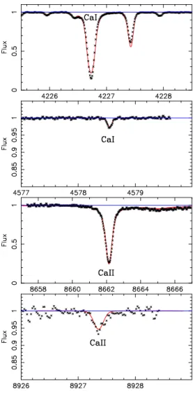
Fig. 1.Profiles of Ca I and Ca II lines in Procyon. The wavelengths are in Å. The small crosses represent the observed spectrum and the (red) line the computed profile. With our model atom, the observed and computed profiles of the Ca I and Ca II lines agree well.

3.3. Consistency check

To test the Ca atom model, we computed the profiles of the calcium lines in the Sun, in Procyon, and in two classical metal-poor stars HD 122563, and HD 140283. The synthetic spectra were computed following the procedure described in Korotin (2008): we calculated the departure coefficients factors “b” for the Ca lines with MULTI and then used these factors in the LTE synthetic spectrum code.

•For the Sun we used the solar atmosphere model com-puted by Castelli with a chromospheric contribution following Vernazza et al. (1981) (see section 3.1). A micro turbulence velocity ξt=1.0 kms−1 was adopted in the atmosphere.

We computed the profile of 49 lines of CaI and 17 lines of CaII. The log g f value of the lines and the broadening pa-rameter due to collisions with hydrogen atoms, log γVW/NH

(for T=10 000K), are given in Table 2. We found log ǫ(Ca) = 6.31 ± 0.05 from the CaI lines and log ǫ(Ca) = 6.30 ± 0.07 from the CaII lines. These values agree well with the mete-oritic calcium abundance log ǫ(Ca) = 6.31 ± 0.02 (Lodders et

Fig. 2.Profiles of Ca I and Ca II lines in HD 140283. The wavelengths are in Å. The symbols are the same as in Fig. 1. The observed spectrum and the synthetic profiles computed with log ǫ(Ca) =4.12 agree well.

al., 2009) and the photospheric abundances derived by Asplund et al. (2009) for the solar atmosphere: log ǫ(Ca) = 6.34 ± 0.04 (a value that includes 3D effects).

For most of the lines in Table 2, the broadening parameter log γVW/NH (for T=10 000K) due to collisions with hydrogen

atoms, was taken from the precise calculations of Anstee & O’Mara (1995), Barklem & O’Mara (1997, 1998), and Barklem et al. (1998). For the other lines, this parameter was derived from the fit of the solar atlas (Kurucz et al., 1984). These values are, for the high excitation lines of CaII, higher than the values obtained from the Uns¨old or Kurucz approxi-mation. However, they agree well with the values obtained by Ivanova et al. (2002), who note that the use of the Uns¨old or Kurucz approximation often leads to an underestimation of the broadening parameter.

• We retrieved the spectrum of Procyon from the UVES POP (Bagnulo et al., 2003). Procyon has a solar-like chemical composition, and its surface gravity, derived from Hipparcos measurements (Perryman et al., 1997), is log g=3.96. We adopted a microturbulence ξt =1.8 kms−1. For this star,

Spite et al.: NLTE determination of the abundance of Calcium in EMP stars 5 Table 2.Parameters of the Ca lines used in the solar spectrum. γ1 =

log γVW/NHfor a temperature of 10 000K.

line log g f γ1 line log g f γ1

(nm) Ref Ref (nm) Ref Ref

Ca I Ca I 410.8526 -0.824 1 -6.97 11 616.6439 -1.143 4 -7.15 9 422.6728 0.244 6 -7.56 9 616.9042 -0.797 4 -7.15 9 428.3011 -0.220 3 -7.50 12 616.9563 -0.478 4 -7.15 9 428.9367 -0.300 3 -7.50 12 643.9075 0.390 4 -7.57 9 430.2528 0.280 3 -7.50 12 645.5598 -1.340 2 -7.65 1 431.8652 -0.211 3 -7.50 12 646.2567 0.262 4 -7.57 9 435.5079 -0.420 3 -6.80 11 647.1662 -0.686 4 -7.57 9 442.5437 -0.360 3 -7.16 9 649.3781 -0.109 4 -7.57 9 443.4957 -0.010 3 -7.16 9 649.9650 -0.818 4 -7.57 9 443.5679 -0.523 3 -7.16 9 657.2779 -4.296 6 -7.69 9 445.4779 0.260 3 -7.16 9 671.7681 -0.523 4 -7.14 9 445.6616 -1.660 3 -7.16 9 714.8150 0.137 4 -7.80 1 451.2268 -1.892 4 -7.26 1 720.2200 -0.262 7 -7.80 1 452.6928 -0.548 4 -7.00 11 732.6145 -0.208 7 -7.30 11 457.8551 -0.697 4 -7.00 11 1034.3820 -0.409 5 -7.12 9 468.5268 -0.880 3 -6.40 11 518.8844 -0.115 4 -7.00 11 Ca II 526.0387 -1.719 4 -7.51 9 393.3663 0.104 6 -7.76 9 526.1704 -0.579 4 -7.51 9 396.8469 -0.201 6 -7.76 9 526.5556 -0.114 4 -7.51 9 500.1479 -0.506 10 -7.34 1 534.9465 -0.310 4 -7.44 12 645.6875 0.412 10 -6.61 11 551.2980 -0.464 7 -7.00 11 820.1722 0.300 2 -7.00 11 558.1965 -0.555 4 -7.54 9 824.8796 0.570 2 -7.00 11 558.8749 0.358 4 -7.54 9 825.4730 -0.400 2 -7.00 11 559.0114 -0.571 4 -7.54 9 849.8023 -1.416 8 -7.68 9 559.4462 0.097 4 -7.54 9 854.2091 -0.463 8 -7.68 9 585.7451 0.240 4 -7.12 11 866.2141 -0.723 8 -7.68 9 586.7562 -1.570 7 -7.00 11 891.2068 0.631 10 -7.21 11 610.2723 -0.770 4 -7.19 9 892.7356 0.808 10 -7.21 11 612.2217 -0.319 4 -7.19 9 985.4759 -0.228 10 -7.00 11 615.6023 -2.497 5 -7.15 9 989.0628 1.270 10 -7.01 11 616.1297 -1.268 4 -7.15 9 993.1374 0.051 2 -7.00 11 616.2173 -0.090 3 -7.19 9 1183.8997 0.290 2 -7.36 11 616.3755 -1.286 7 -7.15 9 1194.9745 -0.010 2 -7.36 11 References

1: VALD 2: Wiese et al. (1969)

3: Wiese & Martin (1980) 4: Smith & Raggett (1981) 5: Kurucz & Bell (1995) 6: Morton (1991)

7: Smith et al. (1988) 8: Theodosiou (1989)

9: Anstee & O’Mara (1995), Barklem & O’Mara (1997,1998) 10: Opacity project 11: fit of the Solar atlas 12: Uns¨old formula + fit of the Solar atlas

et al., 2003) or Teff= 6590 K (Korn et al., 2003) found a

subsolar abundance of Ca and a difference of about 0.2 dex between the NLTE calcium abundance derived from the CaI and CaII lines.

With Teff=6510 K and our model atom, we derive for Procyon

a near solar calcium abundance and a much better agreement between CaI and CaII: log ǫ(Ca) = 6.25 ±0.04 from CaIlines and 6.27 ±0.06 from CaIIlines (Fig. 1).

• We also tested our model on two classical metal-poor stars: HD 122563 (a star from our sample of giants) and HD 140283. The spectrum of HD 140283 was retrieved from the ESO POP (Bagnulo et al., 2003). For HD 122563 we adopted the parameters given in Table 1, and for HD 140283 the parameters given by Hosford et al. (2009): Teff=5750 K,

log g=3.4, ξt=1.5 kms−1. The agreement is good. From the

CaI lines we obtain log ǫ(Ca) = 4.12 ± 0.04 and from the CaIIlines log ǫ(Ca) = 4.08 ± 0.05. In Fig. 2 we show the fit be-tween the observed spectrum of HD 140283 and the synthetic profiles computed with log ǫ(Ca) = 4.12.

Fig. 3. Profiles of three Ca lines computed for a giant star with [Ca/H] ≈ −2.5 with LTE (thin blue line) and NLTE (thick red line) hypotheses. The wavelengths are given in Å.

a) The NLTE profile of the Ca I resonance line is narrower in the wings and deeper in the core. b) In a Ca I subordinate line, for the same abundance of calcium the equivalent width computed under the NLTE hypothesis is slightly smaller. c) The NLTE correction is im-portant for the strong IR Ca II line (note that the scale in wavelength is different for this line), but the wings are not affected and a reliable calcium abundance can be deduced from these wings via LTE analy-sis.

4. Calcium abundance in the EMP stars sample

4.1. Comparison between the different systems

In Fig.3 we show the influence of the NLTE effects on the profile of some typical calcium lines measurable in extremely metal-poor stars. Evidently, in particular the wings of the lines of the CaII infrared triplet are not sensitive to NLTE effects until the wings are strong enough.

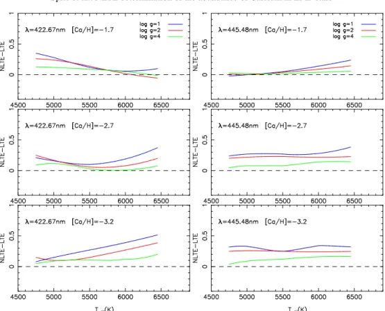
In Fig. 4 the correction NLTE-LTE is given as a funtion of the temperature, the gravity, and the calcium abundance for the CaI resonance line and a typical subordinate line of CaI. The NLTE corrections for different temperatures, gravities, and abundances for all the Ca lines used in this analysis (Table 2) are available in electronic form2_{. The influence of the complex}

NLTE effects as a function of the stellar parameters and of the characteristics of the lines has been discussed by Mashonkina et al. (2007) and Merle et al. (2011).

Fig. 4.NLTE corrections for the Ca I resonance line at 422.67 nm and for a typical subordinate line of Ca I at 445.48 nm.

In Table 1 we give for each star the mean abundance de-rived from the subordinate lines of CaI (col. 6), the number of lines used for the analysis (col. 7), and the internal error (col. 8). Column 9 lists the abundance deduced from the res-onance line of CaI, and column 10 the abundance computed from the infra-red CaII line at 866.21nm (only this line of the red CaIItriplet is in the wavelength range of our spectra). Columns 11 and 12 list [Ca/H] and [Ca/Fe] deduced from the subordinate lines of CaI. For an easier comparison to the pre-vious “First Stars” papers, the solar abundance of calcium was taken from Grevesse & Sauval (2000) as in Cayrel et al. (2004): logǫ(Ca) ⊙ =6.36. The oscillator strengths of the calcium lines measured in our metal-poor stars were updated (to be the same as in section 3.2). As a consequence, for some lines (Table 2) they are slightly different from the log g f values used in Cayrel et al. (2004) and Bonifacio et al. (2009).

The abundance of Ca was deduced from the equivalent widths for the subordinate lines of CaI. But for the

reso-nance line, which is often strong and slightly blended with FeI

and CH lines, a fit of the profile was made.

The Ca abundance was generally deduced from a fit of the wings (insensitive to NLTE effects) for the red CaII lines.

However, in the turnoff stars and in the most metal-poor gi-ants, the wings almost disappear (when the equivalent widths are less than 400 mÅ) and in this case, equivalent widths were used.

In Fig. 5 we compare the abundances of calcium derived from these different systems. The abundance deduced from the line of the infrared triplet of CaII at 862.21nm is, as a mean, 0.07 dex lower than the abundance deduced from the

subor-dinate lines of CaI (Fig. 5a). This small difference is quite satisfactory since the abundance deduced from the CaII lines depends on the surface gravity of the model, and this gravity can be affected by a systematic error since it has been derived from the ionization equilibrium of iron under the LTE hypoth-esis (see Cayrel et al., 2004).

In Fig 5b, the calcium abundance derived from the subordi-nate lines of CaI is compared to the abundance deduced from the CaIresonance line at 422.67nm. It is well known that in very metal-poor stars, under the LTE hypothesis, this resonance line leads to an underestimation of the calcium abundance: e.g. Magain (1988), Ryan et al. (1996). But it was expected that NLTE computations of the lines would remove this effect. For one typical metal-poor giant CS 22172-02 we show in Fig. 6 the observed spectrum and theoretical spectra computed with abundances log ǫ(Ca) = 2.52 (best fit), 2.8 and 3.1. The subor-dinate lines lead to a Ca abundance of 3.11; this value is well established: seven of the subordinate lines have an equivalent width stronger than 9 mÅ and the scatter in abundance is only 0.09 dex.

A similar discrepancy has been observed, after NLTE com-putations, in several metal-poor stars by Mashonkina et al. (2007) and the authors suggested that the explanation could lie with the 1D atmospheric models adopted for the computations, since the CaI resonance line is formed over a more extended range of atmospheric depths than the subordinate lines.

Spite et al.: NLTE determination of the abundance of Calcium in EMP stars 7

Fig. 5.Difference between [Ca/H] deduced from the subordinate lines of Ca I and [Ca/H] deduced from a) the infrared triplet of Ca II and b) the resonance line of Ca I. The filled circles represent the turnoff stars and the open symbols the giants. The error bar on [Ca/H], ∆Ca 866.21 and ∆ Ca 422.67 is generally less than 0.1dex. It is indi-cated only when it exceeds 0.1dex.

a) The Ca abundance deduced from the line of the infrared triplet is, as a mean, 0.07 dex lower than the abundance derived from the subor-dinate lines of Ca I.

b) For [Ca/H] ≈ −2, the abundance deduced from the Ca I resonance line agrees quite well with the abundances deduced from subordinate lines, but a discrepancy appears and increases linearly when [Ca/H] decreases. It reaches about 0.4 dex for [Ca/H]= –3.5.

Fig. 6.Observed profile of the resonance line of Ca I (crosses) for one typical metal-poor giant compared to theoretical profiles com-puted with log ǫ(Ca) = 2.52 (thick red line), 2.8 and 3.1 (thin blue lines). The wavelengths are in Å. The (very small) difference between the observed spectrum and the profile computed with log ǫ(Ca) = 2.52 is shown at the bottom of the figure (dots, shifted by 0.1). For this star, the subordinate lines lead to log ǫ(Ca) = 3.11 (Table 1).

4.2. Influence of convection - 3D models 4.2.1. Shift of the calcium lines

The atmospheres of cool stars are not static. Velocity and in-tensity fluctuations caused by convection are observed in the Sun (Rutten et al., 2004) and in metal-poor stars. Ram´ırez et al. (2010) found that in HD 122563 (a star of our sample of giants) the cores of the FeI lines are shifted relative to the mean ra-dial velocity of the star, this shift increases with the equivalent width of the line. Weaker lines form in deeper layers, where the

granulation velocities and intensity contrast are higher. We also observe this phenomenon for the calcium lines in all stars of our sample. The radial velocity of the stars were determined from a constant set of iron lines, and relative to this “zero point”, the radial velocity derived from the CaI resonance line is about 0.4 kms−1 _{higher in the giants and 0.2 kms}−1 _{higher in the}

dwarfs. In contrast, the radial velocity derived from the (weak) subordinate calcium lines is about 0.4 kms−1 _{lower in the}

gi-ants and about 0.2 kms−1 _{lower in the dwarfs. (We were able}

to measure precisely the shift of the subordinate lines only on the “blue spectra” when these lines were larger than 20 mÅ.) At the resolution of our VLT/UVES spectra with R ≈ 45000, the asymmetry of the lines cannot be reliably measured.

The shift of the CaI resonance line does not clearly depend on [Ca/H], and therefore it does not seem that there is a clear correlation between the shift of the Ca lines and the discrep-ancy between the abundances deduced from the resonance or the subordinate lines.

4.2.2. Abundance correction

The largest abundance corrections caused by granulation ef-fects occur at low metallicities. This is mainly because the dif-ference between the 1D and 3D predictions for the mean tem-perature of the outer layers of metal-poor stars is very large (see e.g. Gonz´alez Hern´andez et al., 2010). We tried to investigate the change in abundances caused by thermal inhomogeneities and differences in formation depth (3D corrections hereafter) for the CaIresonance line at 422.67 nm and for a typical sub-ordinate line of CaI at 445.48 nm.

–For a representative turnoff star, we used a 3D-CO5BOLD model (Freytag et al., 2002, 2011) from the CIFIST grid (see Ludwig et al., 2009) with parameters (Teff, log g, [Fe/H]):

6270 K/4.0/–3.0).

–For the giants we used two models (4488 K/2.0/–3.0 and 5020 K/2.5/–3.0) from the CIFIST grid. They have both a grav-ity slightly higher than the ones in our sample of giants, but no closer 3D model is available at the moment.

From these computations we found that for [Fe/H]=–3, [Ca/H]=–2.6, the 3D correction for the subordinate lines of CaI in turnoff and in giant stars is very small.

In giants, the 3D correction seems to be negligible also for the resonance line. But with the model of turnoff stars, we found for the resonance line a 3D correction of –0.44 dex, and there-fore the 3D correction increases the discrepancy between the subordinate lines and the 422.67 resonance line.

To date, it is not well understood why the abundance of calcium deduced from the resonance line of CaI is at very low metallicity, lower than the abundance deduced from the subor-dinate lines. It would be interesting to repeat the 3D compu-tations with more metal-poor models (not available today). A fully consistent 3D NLTE model atmosphere and line forma-tion scheme is currently beyond our reach.

5. Results and discussion

In this section we adopt the Ca abundance deduced from the subordinate lines of CaI (Tab. 1, columns 11 and 12).

Fig. 7.[Ca/Fe] vs. [Fe/H] in our sample of EMP stars. Symbols as in Fig 5. Turnoff and giant stars agrees quite well, [Ca/Fe] is constant in the range −4.3 < [Fe/H] < −2.5 and the mean value is equal to [Ca/Fe]=0.5, a value slightly higher than the LTE value [Ca/Fe]=0.35 (see Bonifacio et al., 2009).

In Fig. 7 we present the new relation between [Ca/Fe] and [Fe/H]. The error bar plotted in for the subordinate lines the fig-ure is the quadratic sum of the error due to the uncertainty of the model and the random error of the Ca abundance derived from the subordinate lines. The agreement between the turnoff and the giant stars is excellent, the ratio [Ca/Fe] is constant in the interval −4.5 < [Fe/H] < −2.5. The slope of the regression line is –0.05. The scatter of [Ca/Fe] is a little smaller when NLTE effects are taken into account: 0.09 from NLTE computations compared to 0.10 from LTE computation .

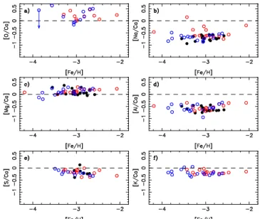
In Fig. 8 we present the behavior of the abundances of O, Na, Mg, Al, S and K relative to Ca. The computation of these abundances take into account the NLTE effects (Andrievsky et al. 2007, 2008, 2010 and Spite et al. 2011). Since the abun-dance of oxygen has been determined from the forbidden oxy-gen line at 630 nm (Cayrel et al. 2004), it is free of NLTE ef-fects.

In Fig. 8, different symbols are used for mixed and unmixed giants. After Spite et al. (2005, 2006) we call “mixed giants”, those where, ownng to mixing with deep layers, carbon has been partially transformed into nitrogen ([C/N] < −0.6), part of 12_{C has been transformed into} 13_{C (}12_C/13_{C < 10), and}

lithium is not detected (lithium has been severely depleted by this mixing). In the HR diagram, these “mixed giants” are lo-cated above the “bump”. It has been found (Andrievsky et al., 2007) that some mixed giants are enriched in sodium, this is visible in Fig. 8b. This Na-enhancement reflects a deep internal mixing (or an AGB status, or a contamination by AGB stars), but it does not reflect an anomaly of the chemical composition of the cloud that formed the star. Therefore the mixed stars can-not be used to determine the ratio [Na/Ca] in the early galactic matter.

Since the abundance ratios of O, Na, Al, S, and K rela-tive to Ca are fairly flat vs. [Fe/H] in the central part of the diagram, we can define a mean value in this central interval, say −3.6 < [Fe/H] < −2.5 as has been done with Mg in Andrievsky et al. (2010). The mean values of [X/Fe], [X/Mg] and [X/Ca] are given in Table 3 with the corresponding scatter. However, an anti-correlation seems to exist between [S/Ca] and [Fe/H] and also [S/Mg] and [Fe/H]: the Kendall τ coefficient is

Fig. 8.Abundance ratios of O, Na, Mg, Al, S, and K relative to Ca in the early Galaxy. The abundances of all these elements were com-puted taking into account the NLTE effect. The black dots represent the turnoff stars, the open circles the giants (blue for the unmixed gi-ants and red for the mixed gigi-ants).

Table 3.Mean value of the ratios [X/Fe], [X/Ca] and [X/Mg] in the interval −3.6 < [Fe/H] < −2.5 and scatter around the mean

X [X/Fe] σFe [X/Mg] σMg [X/Ca] σCa O 0.67 0.17 0.07 0.20 0.23 0.22 Na -0.22 0.11 -0.82 0.14 -0.70 0.11 Mg 0.68 0.13 – – 0.12 0.11 Al -0.10 0.11 -0.71 0.11 -0.58 0.13 S 0.31 0.12 -0.31 0.15 -0.19 0.12 K 0.31 0.09 -0.32 0.15 -0.18 0.10 Ca 0.49 0.10 -0.12 0.11 – –

98.9% for [S/Ca] and 99.1% for [S/Mg]. In these computations the weight of BD +17◦_{3248 ([Fe/H]=–2.2) is important. This}

star is quite peculiar: according to For & Sneden (2010) it is a red horizontal branch star strongly enriched in heavy elements (Cowan et al., 2002). However, if this star is removed from the computations, the Kendall τ coefficient remains high: 97.6% for [S/Ca] and 97.9% for [S/Mg].

One turnoff star, BS 16023-046, and one unmixed giant CS 22956-50, have abnormally strong and broad sodium D lines. Their radial velocity (–7.5 kms−1_{and –0.1 kms}−1_{) is low,}

and the stellar lines are very probably blended with interstellar lines. These stars have not been plotted on Fig. 8b and were not taken into account in computing the mean value and the scatter of [Na/Fe], [Na/Mg] and [Na/Ca] in Table 3.

It is interesting to take advantage of the high quality of the data to compare in Table 3 the scatter around the mean value when Fe, Mg, or Ca are taken as reference elements. The scatter of [O/Fe], [O/Mg] or [O/Ca] is fairly large: about 0.2 dex but this can be explained by the scatter of the oxygen abundance

Spite et al.: NLTE determination of the abundance of Calcium in EMP stars 9

due to the reduced number of oxygen lines and the difficulty of the measurements. For the other ratios the scatter lies be-tween 0.09 and 0.15 dex and we consider that this difference of 0.06 dex is significant. The scatter is always significantly smaller when Ca is taken as the reference element, with two exceptions:

•Oxygen: but in this case we have seen that the scatter is domi-nated by the error on the measurement of the very weak oxygen line.

•Aluminum: Al is better correlated with Mg than with Ca. But this correlation (opposite to the well known anti-correlation found in globular cluster stars) has at least one exception: CS 29516-024 is rather Al-poor but it is (relatively) Ca-rich and Mg-rich, and it does not seem possible to explain these differences by errors of measurements. A similar correlation between [Al/Fe] and [Mg/Fe] has been also suggested by Suda et al. (2011) even in a large but very inhomogeneous sample of metal-poor stars.

6. Concluding remarks

We determined the calcium abundance in a homogeneous sam-ple of of 53 metal-poor stars (31 of them with [Fe/H] < −2.9) taking into account departures from LTE. We have shown that the trend of the ratio [Ca/Fe] vs. [Fe/H], below [Fe/H]=–2.7 is almost flat and derived a new mean value of [Ca/Fe] in the early Galaxy: [Ca/Fe] = 0.5 ± 0.09.

Generally speaking, our NLTE calculations agree quite well with those of Mashonkina et al. (2007). However, Mashonkina et al. had found different Ca abundances from the CaI and CaII lines in Procyon. With our new model atom of cal-cium, we are able to reconcile the calcium abundance deduced from neutral and ionized calcium lines in Procyon. We derived log ǫ(Ca) = 6.25 ±0.04 from CaI lines and 6.27 ±0.06 from CaIIlines (6.33 and 6.40 under the LTE hypothesis). Moreover, the calcium abundance is found to be solar, as expected.

In metal-poor stars (below [Ca/H]=–2.5), a discrepancy clearly appears between the Ca abundances deduced from ei-ther the resonance CaI line, or the CaI subordinate lines. A rough estimation of the effect of convection on the profile of these lines does not explain this discrepancy.

In the stars of our sample (giants and turnoff stars) the wavelengths of the calcium lines are shifted by convection as a function of the equivalent width of the lines as has been found for the iron lines by Ram´ırez et al. (2010) in HD 122563.

The scatter around the mean value of [Ca/Fe] is small but since the NLTE correction is about the same for all the subor-dinate lines used in this analysis, the scatter is almost the same as it was in the LTE analyses (Cayrel et al., 2004, Bonifacio et al., 2009).

The abundance of the light metals O, Na, Al, S, K is well correlated with the calcium abundance. The correlation is gen-erally a little better than it is with the magnesium abundance (with exception of the tight aluminium/magnesium correla-tion). However, it is striking that in Table 3, even when NLTE is taken into account, the correlation of the light elements O, Na, Al, S, K with Ca or Mg (all supposed to be formed mainly by hydrostatic fusion of C, Ne or O), is never better than the

corre-lation with iron, providing some support to supernovae models predicting nucleosynthesis of all these elements predominantly in explosive modes (e.g. Nomoto et al. 2006).

Acknowledgements. The authors thank the referee, who indicated new log g f values for the high excitation Ca II lines. This work has been supported in part by the ”Programme National de Physique Stellaire” (CNRS). S.A. kindly thanks the Observatoire de Paris, the CNRS, and the laboratory GEPI for their hospitality and support during his stay in Meudon. He acknowledges the National Academy of Sciences of Ukraine and the franco-Ukrainian exchange program for its financial support under contract UKR CDIV N24008.

References

Allen C.W., 1973, Astrophysical Quantities, Athlone Press, London Alonso A., Arribas S., Mart´ınez-Roger C., 1996, A&A 313, 873 Alonso A., Arribas S., Mart´ınez-Roger C., 1999, A&AS 140, 261 Alonso A., Arribas S., Mart´ınez-Roger C., 2001, A&AS 376, 1039 Andrievsky S., Spite M., Korotin S. et al., 2007, A&A 464, 1081 Andrievsky S. M., Spite M., Korotin S. A., Spite F., Bonifacio P.,

Cayrel R., Hill V., Franc¸ois P., 2008, A&A 481, 481 Andrievsky S., Spite M., Korotin S. et al., 2010, A&A 509, 88 Anstee S. D., O’Mara B. J., 1995, MNRAS, 276, 859

Asplund M. et al., Grevesse N., Sauval J., Scott P., 2009, ARA&A, 47, 481

Bagnulo S., Jehin E., Ledoux C. et al., 2003, The Messenger, 114, 10 Barklem P. S., O’Mara B. J., 1997, MNRAS 290, 102

Barklem P. S., O’Mara B. J., 1998, MNRAS 300, 863

Barklem P. S., O’Mara B. J., Ross, J. E., 1998, MNRAS 296, 1057 Bonifacio P., Molaro P., Sivarani T. et al., 2007, A&A 462, 851 Bonifacio P., Spite M., Cayrel R. et al., 2009, A&A 501, 519 Burgess,A., Chidichimo M. C., Tully J. A., 1995, A&A 300, 627 Caffau E., Ludwig H.-G., 2007, A&A 467, L11

Carlsson M., 1986, Uppsala Obs. Rep. 33

Cayrel R., Depagne E., Spite M. et al., 2004, A&A 416, 1117 Cowan J.J., Sneden C., Burles S., Ivans I.I., Beers T.C., Truran J.W. et

al., 2002, ApJ 572, 861

Dekker H., D’Odorico S., Kaufer A., Delabre B., Kotzlowski H., 2000, Proc. SPIE 4008, 534

For B.-Q., Sneden C., 2010, AJ 140, 1694

Freytag B., Steffen M., Dorch B., 2002, AN 323, 213

Freytag B., Steffen M., Ludwig H.-G., Wedemeyer-B¨ohm S., Schaffenberger W., Steiner O., 2011, JCoPh, 231, 919

Gonz´alez Hern´andez J.I., Bonifacio P., Ludwig H.-G., Caffau E., Behara N. T., Freytag B., 2010, A&A 519, 46

Grevesse N., Sauval A.J., 2000, ”Origin of the elements in the solar system. Implications of post-1957 Observations”, ed. O. Manuel, Kluwer Academic/Plenum Publishers, p.261

Hirata R., Horaguchi T., 1995, Catalogue of Atomic Spectroscopic Lines, Vol. 6 (Strasbourg : CDS), 69

Hosford A., Ryan S. G., Garca Prez A. E., Norris J. E., Olive K. A., 2009, A&A 493, 601

Ivanova D. V., Sakhibullin N. A., Shimanskii V. V., 2002, ARep 46, 390

Kobayashi Ch., Umeda H., Nomoto K. et al., 2006, ApJ 653, 1145 Korn, A., Shi, J., Gehren, T., 2003, A&A, 407, 691

Korotin S.A., 2008, Odessa Astronomical Pub. 21, 42

Korotin S.A., Andrievsky S.M., Luck R.E., 1999, A&A 351, 168 Kurucz R.L., 1992, RMxAA 23, 181

Kurucz R.L., 1993, SAO, Cambridge, CDROM18 Kurucz R.L., Bell B., 1995, SAO, Cambridge, CDROM23

Kurucz R.L., Furenlid I., Brault J., Testerman L., 1984, National Solar Observatory Atlas, Sunspot, New Mexico: National Solar Observatory, 1984

Lodders K., Plame H., Gail H.-P., 2009, in Landolt-B¨ornstein, New Series, Volume VI/4B Chapter 4.4. Edited by J.E. Tr¨umper, Berlin Heifelberg New York: Springer-Verlag p. 560

Ludwig H.-G., Behara N. T., Steffen M., Bonifacio P., 2009, A&A 502, 1L

Magain P., 1988, in IAU Symp 132, “The impact of Very High S/N spectroscopy on Stellar Physics”, G. Cayrel de Strobel & M. Spite eds (Dordrecht, Kluwer) p.485

Mashonkina L., Gehren T., Travaglio C., Borkova T., 2003, A&A, 397, 275

Mashonkina L., Korn A.J., Przybilla N., 2007, A&A 461, 261 Mel´endez M., Bautista M.A., Badnell N.R., 2007, A&A 469, 1203 Merle T., Th´evenin F., Pichon B., Bigot L., 2011, MNRAS 418, 863 Morton D.C., 1991, ApJS 77,119

Nomoto K., Tominaga N., Umeda H. et al., 2006, Nucl. Phys. A 777, 424

Perryman M. A. C., Lindegren L., Kovalevsky J. et al., 1997, A&A, 323, L49

Ram´ırez I., Collet R., Lambert D.L., Allende Prieto C., Asplund M., 2010, ApJL 725, L223

Rutten R. J., Hammerschlag R. H., Bettonvil F. C. M., S¨utterlin P., & de Wijn A. G., 2004, A&A 413, 1183

Ryan S.G., Norris J.E., Beers T.C., 1996, ApJ 471, 1996 Samson A. M., Berrington K. A., 2001, ADNDT 77, 87

Seaton M.J., 1962, in Atomic and Molecular processes (New York: Academic Press)

Smith G., 1988, J. Phys. B, 21, 2827

Smith G., Raggett D. St. J., 1981, J. Phys. B, 14, 4015 Spite M., Cayrel R., Plez B. et al., 2005, A&A 430, 655 Spite M., Cayrel R., Hill V. et al., 2006, A&A 455, 291 Spite M., Caffau E., Andrievsky S. et al., 2011, A&A 528, 9 Steenbock W., Holweger H., 1984, A&A 130, 319

Suda T., Yamada S., Katsuta Y., Komiya Y. et al., 2011, MNRAS 412, 843

Sugar J., Corliss C., 1985, J. Phys. Chem. Ref. Data, 14, Suppl. No. 2 Theodosiou C. E., 1989, Phys. Rev. A, 39, 4880

Van Regemorter H., 1962, ApJ 136, 906

Vernazza J. E., Avrett E. H., Loeser R., 1981, ApJS, 45, 635 Wiese W.L., Martin G.A., 1980, NSRDS-NBS 68, Part II