Computing 3-D motion in custom analog and digital VLSI

Computing 3-D Motion in Custom Analog

and Digital VLSI

by

Lisa G. Dron

S.B., Massachusetts Institute of Technology (1976)

M.S.E., University of Texas at Austin (1989)

Submitted to the Department of Electrical Engineering and Computer Science

in partial fulfillment of the requirements for the degree of

Doctor of Philosophy

at the

Massachusetts Institute of Technology

September 1994

@ Lisa G. Dron, 1994

The author hereby grants to MIT permission to reproduce and to

distribute publicly paper and electronic copies of this thesis

document in whole or in part.

eiS nature

of Anthor

Department of Electrical Engineering and Computer

August

A ece,nted 1w~

V

-Berthold

K. P. Horn

Prof~ssor of CQmiauter Science and Engineering

7;Tlhesis Supervisor

N . -..-.... --.... ---.

r C...aC

h deric R. Morgenthaler Chairman, Depart ental Commit ee on Graduate Students

8. ! :• i

Science

9, 1994

U^~--~V C1~rt;f~e.d

C

ertfie b

by Accente .. b _...

Computing 3-D Motion in Custom Analog and Digital VLSI

by

Lisa G. Dron

Submitted to the Department of Electrical Engineering and Computer Science on August 9, 1994, in partial fulfillment of the

requirements for the degree of Doctor of Philosophy Abstract

Computing the general 3-D motion of a camera from the changes in its images as it moves through the environment is an important problem in autonomous navigation and in machine vision in general. The goal of this research has been to establish the complete design framework for a small, autonomous system with specialized analog and digital VLSI hardware for computing 3-D camera motion in real-time. Such a system would be suitable for mounting on mobile or remote platforms that cannot be tethered to a computer and for which the size, weight and power consumption of the components are critical factors.

Combining algorithmic design with circuit design is essential for building a robust size-and power-efficient system, as there are constraints imposed both by technology size-and by the nature of the problem which can be more efficiently satisfied jointly. The first part of this thesis is thus devoted to the analysis and development of the algorithms used in the system and implemented by the special processors. Among the major theoretical results presented in Part I are the development of the multi-scale veto edge detection algorithm, the derivation of a simplified method for solving the motion equations, and a complete analysis of the effects of measurement errors on the reliability of the motion estimates.

In the proposed system architecture, the first step is to determine point correspondences between two successive images. Two specialized processors, the first a CCD array edge de-tector implementing the multi-scale veto algorithm, and the second a mixed analog/digital binary block correlator, are proposed and designed for this task. A prototype CCD edge detector was fabricated through MOSIS, and based on the test results from this chip, im-provements are suggested so that a full-size focal-plane processor can be built. The design of the mixed analog/digital correlator is compared with a fully digital implementation and is seen to yield a significant reduction in silicon area without compromising operating speed. In the conclusions, the theoretical and experimental results from the different parts of this thesis are combined into a single design proposal for the complete motion system.

Thesis Supervisor: Berthold K. P. Horn

Acknowledgments

My years at MIT would not have been as meaningful without the help, support, and advice of many people. I would first like to thank my thesis advisor Berthold Horn for the complete freedom he gave me to pursue the research I was interested in, and I am grateful to my other committee members, Charlie Sodini and Jim Roberge, for their time spent in reading this thesis and for their helpful comments along the way.

I wish to give special thanks to the other present and former members of the Analog VLSI for Machine Vision group: Ig McQuirk, Steve Decker, Chris Umminger, Craig Keast, Mikko Hakkarainen, and John Harris who provided much needed technical advice and help. Spe-cial thanks also goes to my graduate counselor, Jacob White, for years of helpful advice that was never judgemental or critical-even when he was telling me I was wrong.

I certainly could have never gotten as much done without the help of three special support staff members of the AI Lab. Ron Wiken was always there to help me find or build ev-erything I needed. Bruce Walton kept the computers running, and regardless of how much direct help he gave me on my thesis, he deserves to be acknowledged as the friendliest and most patient system manager I have ever known in my life. Laurel Simmons facilitated everything, from bringing in electricians when I needed them, to soldering the bulkhead connectors in the Vision Lab, to letting me take home all of my equipment this past year so that I could spend more time with my family and still graduate. In addition to these three, Eric Grimson patiently supported everything I did, from Vision Night 92, to letting me set up the Vision Lab the way I wanted to.

I owe a tremendous debt to AT&T Bell Labs for supporting me under their GRPW fel-lowship program for the last five years. Almost as important as the financial support was the real personal support I received from my mentor, Behrokh Samadi, and from Dexter Johnston. I also owe a great deal to Chuck McCallum for sponsoring my candidacy to the program. I only hope he is not still disappointed that I didn't go into Operations Research.

Finally, my deepest appreciation goes to those who are closest to me: to my sons, David and William, who have now spent half their lives watching their mother go through graduate school; and to Michael, whose love and support made everything possible.

This thesis describes research done at the Artificial Intelligence Laboratory of the Massachusetts Institute of Technology in collaboration with the Analog VLSI for Machine Vision research project. Support for the Laboratory's research is provided in part by the ARPA contract N00014-85-K-0124. Funding for the Analog VLSI for Machine Vision research project is provided by NSF Grant MIP-91-17724 and NSF and ARPA contracts MIP-88-14612. The author has been supported by a GRPW fellowship from AT&T Bell Laboratories.

7

Contents

1 Introduction

I Algorithms and Theory

2 Methods for Computing Motion and Structure

2.1 Basic Equations ...

2.1.1 Perspective geometry... 2.1.2 The epipolar constraint ...

2.2 Computing Motion by Matching Features... 2.2.1 Representing rotation . . . .

2.2.2 Exact solution of the motion equations . . . 2.2.3 Least-squares methods ...

2.3 Correspondenceless Methods ... 2.3.1 Optical flow ...

2.3.2 Direct methods ... . 2.3.3 Limitations of correspondenceless methods 2.4 Motion Vision and VLSI ...

3 Matching Points in Images

3.1 Brightness-Based Methods . . . . 3.2 Gray-level Correlation Techniques . . . . 3.3 Edge-Based Methods . . . . 4 System Architecture 23

24

. . . . 25 S... 25 . . . . 27 S . . . . . . 29 S. . . . . . 30 S . . . . . 32 . . . .. . . . .. . 34

.. .. . .. .. . .

37

. .. .. .. .. . .

38

*. . . . . 39

S . . . .

.

40

. .. . .. .. .. .

45

48 48 50 54

5 An 5.1 5.2 5.3 5.4 5.5

Algorithm for an Analog Edge Detector The Multi-Scale Veto Rule ...

Other Methods and the Use of Multiple Scales

Circuit Models ...

Choosing the Parameters . . . .

Simulations . . .

6 The Matching Procedure

6.1 Finding the Best Match . . . . . .

6.2 Other Tests ... . .

6.3 Simulations . . . . ..

7 Solving the Motion Equations

7.1 The Simplified Algorithm . . . . . .

7.1.1 Pure translation or known rotation 7.1.2 Rotation with known translation . 7.1.3 Pure rotation (Ibi = 0) ...

7.1.4 The complete algorithm . . . .

7.2 Ambiguities and Multiple Solutions . . . .

7.3 Simulations . . . . . 8 The Effects of Measurement Errors

8.1 Numerical Stability . . . . ...

8.1.1 Eigenvalues and eigenvectors of C

8.1.2 Condition of the matrix A. . . . . 8.1.3 Minimizers of S . . .. . . .

8.2 Error Analysis . . . . . 8.2.1

8.2.2 8.2.3

First-order error in the baseline (rotation known) First-order error in the rotation (baseline known)

Coupling between estimation errors . . . . . .

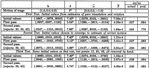
8.3 Experimental Verification 9 Summary of Part I 99 104 105 106 109 113 120 122 128 134 138 150

CONTENTS

II

Design of a CCD-CMOS Multi-Scale Veto Chip

153

10 Basic Requirements

154

11 Charge Coupled Device Fundamentals

156

11.1 Surface Channel Devices ... ... 156

11.2 Buried Channel Devices (BCCDs) ... ... 158

11.3 Charge Transfer and Clocking .. ... 166

11.4 Transfer Efficiency ... 168

11.5 Power Dissipation . . . . ... ... ... 170

11.5.1 On-chip dissipation ... 170

11.5.2 Power dissipation in the clock drivers ...

...

.. . . 171

11.6 Charge Input and Output ... 172

11.6.1 Fill-and-Spill input method ... 172

11.6.2 Floating gate amplifier output structures . . . . . . . .. . 175

12 CCD Edge Detector Design 179 12.1 CCD Processing Array ... 180

12.1.1 Charge sensing ... 183

12.1.2 Clock sequences . . . . . ... ... 187

12.1.3 Boundary processing and charge input . ... 192

12.2 Edge Detection Circuit ... . . . . 197

12.2.1 Double-ended differential amplifier . ... 198

12.2.2 Comparator circuit ... 201

12.2.3 Edge storage ... 204

13 Edge Detector Test Results 206 13.1 Test System ... 209

13.2 Driving Signals Off-Chip ... ... 212

13.3 CCD Tests ... ... .. 215

13.3.1 Channel potential measurements . ... . 215

13.3.2 Input and output ... 217

13.3.3 Dark current measurements ... .... 220

13.4 Differencing and Threshold Test Circuits .... . 13.4.1 Differential amplifier ...

13.4.2 Sense amplifier voltage comparator . . . . 13.4.3 Combined edge veto test circuit... 13.5 Operation of the Full Array Processors . . . . 13.6 Recommendations for Improving the Design . . .

III A Mixed Analog/Digital Edge Correlator

14 Design Specifications

14.1 Required Block Size . . . .. . . . 14.2 Required Search Area ...

14.3 Precision ...

15 Case Study: A Purely Digital Design 15.1 First Method: Moving the Search Window . 15.2 Second Method: One Processor Per Offset . . . .

16 Mixing Analog and Digital

16.1 Unit Cell Design ...

16.2 Global Test Circuits . . . . 16.2.1 Current scaling and conversion . . 16.2.2 Validation and Vmin tests . . . . . 16.3 Test Pattern Simulation . . . . 16.4 Comparison with Digital Architectures .

IV

Conclusions

17 Recommendations for Putting It All Together

224 224 227 228 230 237 240 241 243 244 246 248 249 253 260 262 266 266 270 274 279

281

282 ... . . . . . . . . . . . . . . . . . . . . . . . . . .

CONTENTS

Bibliography

286

Appendices

296

A Quaternion Algebra

297

B Special Integrals

300

B.1 J

lIIe'

e/ d da .. ... 301 B.2 JJI £'14

d

da ... 302

B.3

J~ I'

T

d da

...

302

B.4 JJI 'J1112e IT d da ... 303

B.5

(u

j')l'IT

dd

da. ...

304

B.6 J (u

l')(u2

l')'IT

d da

...

305

2-1 Geometry of perspective projection ... ... . 26

2-2 Epipolar geometry. ... 29

3-1 Example of matching edges despite foreshortening. . ... . 55

4-1 System block diagram ... ... 59

5-1 Results of applying the multi-scale veto rule to an ideal step edge and to an impulse ... . . . 65

5-2 1-D resistive smoothing network with controllable space constant. .... . 69

5-3 2-D MSV edge detection array using charge-coupled devices (CCDs) . . . 70

5-4 Conceptual model of the 'Edge precharge circuit'. . ... . 71

5-5 Ideal 2-D image features ... 74

5-6 Simulated motion sequence: Frontal plane at 10 (baseline) units. Motion is given by: b = (1,0,0), = 50, = (0,1,0). ... 77

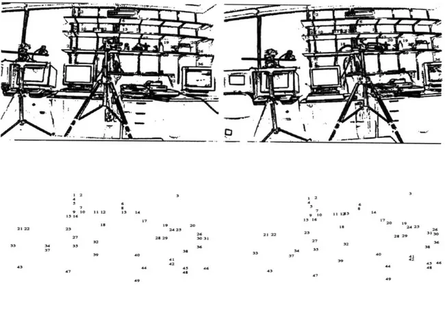
5-7 Real motion sequence: Motion with respect to motion stage coordinate system (not camera system): b = (1, 0, 0), 0 = 50, W = (0, 0, 1). . . .... 78

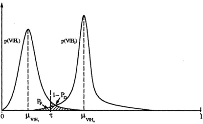
6-1 Threshold selection for a decision rule that chooses between two hypotheses

H

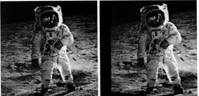
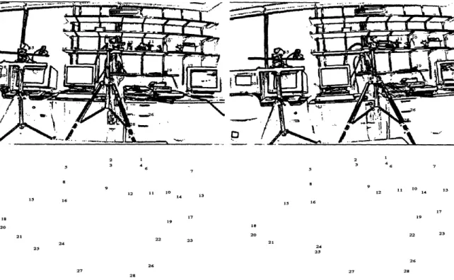
0 and H . ... ... ... . . . . 81

6-2 Binary edge maps of astronaut sequence with correspondence points found by the matching procedure. ... . . ... 86

6-3 Binary edge maps of real motion sequence (lab scene) with correspondence points found by the matching procedure. ... 87 7-1 Binary edge maps of real motion sequence with hand picked point matches. 103

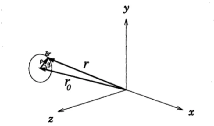
8-1 Geometry of the position vector for a point on the image plane and cone of all vectors for a given field of view. ...

8-2 Change in ri caused by error in determining the exact location of the cor-respondence with the left image. ...

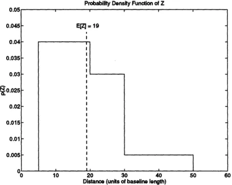
8-3 Probability density function used to obtain random Z values . . . . . 8-4 Estimation errors in translation and rotation with b ± v3 (uncorrelated

measurement errors). b = (1,0,0), 1 = (0,0, 1), 0 = 50 8-5 Estimation errors in translation and rotation with b |j

measurement errors). b = (0, 0, 1),

W

= (0,0, 1), 0 = 50

8-6 Actual and predicted values of /.2/p3 for b 1 b3, for

q

=

with N = 50 and N = 100...

8-7 Actual and predicted values of A 2/ 3 for b

11

%3, for 0 =

with N = 50 and N = 100 ...

8-8 Errors in estimates of translation and rotation with b measurement errors). b = (1, 0, 0), ~i = (0, 0, 1), 8 = 50.

8-9 Errors in estimates of translation and rotation with b measurement errors). b = (0, 0, 1), W = (0,0, 1), 8 = 5°. v3 (uncorrelated 20., 40. , and 600 200, 400, and 600 .I 3 (Systematic. 1 v3 (Systematic v3 (Systematic

'Bucket brigade' analogy of charge coupled devices . . . . . The MOS capacitor. ...

States of the MOS capacitor. ...

Potential profile with depth of a buried channel CCD . . . . Lumped capacitance model of a BCCD . . . . Charge density profile of a buried channel CCD with signal charge (using depletion approximation) ...

Charge transfer sequence with four-phase clocking. ... . . . . Fill-and-spill method for charge input . . . . Charge sensing using the floating gate technique . . . .

Qsig

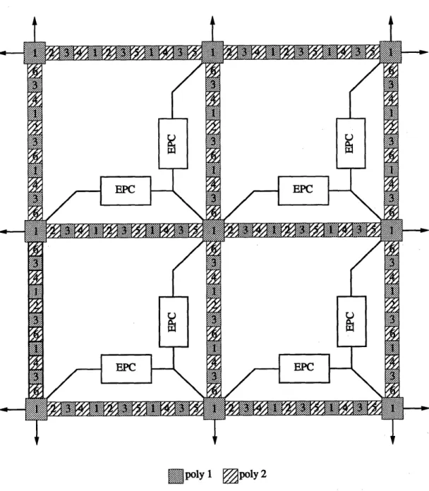
Floor plan of the complete MSV processor . . . . . . Unit cell architecture. ...

Unit cell layout ...

Floating gate design . . . . .

105 121 139 141 142 143 144 147 148 157 158 159 160 161 163 167 173 176 180 181 182 183

LIST OF FIGURES

11-1 11-2 11-3 11-4 11-5 11-6 11-7 11-8 11-9 12-1 12-2 12-3 12-4

12-5 Simulated source follower characteristic for floating gate amplifier (Vbias = 12-6 12-7 12-8 12-9 12-10 12-11 12-12 12-13 12-14 12-15 12-16 12-17 12-18 12-19 12-20 1V ). . . . ... . . . .. . . . .

Charge averaging operation ...

Backspill caused by potential mismatch . . . . . Level shift circuit for correcting potential mismatch problem . . . . . Boundary cell design (north). ...

Boundary cell design (east) ... Boundary cell design (west) ...

CCD input structure... . . . ...

layout of the fill-and-spill structure. . . . .. . . Multi-scale veto edge detection circuit block diagram . . . . .

Clock waveforms for driving edge detection circuit . . . . . Differential amplifier circuit . . . . .

Simulated differential amplifier characteristic for common mode voltages

V,

= 1.2V, 2.OV, and 2.8V (Vbias = 1V). ...

Sense amplifier voltage comparator for threshold tests . . . . . Sense amplifier response with resolution of 6 = 10mV . . . . . Edge charge storage latch ...

13-1 Die photograph of 32x32 array ...

13-2 Die photograph of the test structures chip . . . . . . . 13-3 Test system design ...

13-4 Clock driver circuit used in the test system . . . . 13-5 Analog output pad driver circuit ...

13-6 Analog output pad driver characteristic - simulated vs. actual 1.2V, Vhih = 3.8V). ...

13-7 CCD channel potentials (4-27-94 run) . . . . . 13-8 CCD channel potentials (10-28-93 run) . . . . . . . . .

13-9 Measured source follower characteristic for floating gate amplifier (Vbias = 1V). ... . . . . .. .. . 13-10 Measured floating gate amplifier output vs. fill-and-spill input, Vin - VTef.

13-11 Dark current accumulation for cooled and uncooled chips . . . . . 13-12 Charge transfer efficiency measurement . . . . .

186 188 191 191 193 193 194 195 195 197 198 199 199 202 202 204 207 208 210 212 213 214 216 216 218 219 221 223

LIST OF FIGURES

13-13 Measured differential amplifier characteristic for common mode voltages

V = 1.2V, 2.OV, and 2.8V with Vbias = 1V .

. . . .

. . . ... 225

13-14 Combined maximum differential amplifier outputs vs. IV1 - V21 for common mode voltages

V

c = 1.2V, 2.OV, and 2.8V with Vbias = 1V. . . . . . . . 226

13-15 Measured sense amplifier switching characteristic. . ... 227

13-16 Measured response of one absolute-value-of-difference circuit. . ... . 229

13-17 Measured response of one absolute-value-of-difference circuit, plotted against IV1 - V21. ... ... .. 229

13-18 Composite response of twelve AVD circuits. . ... . 231

13-19 Floating-gate outputs of 4x4 array processor. . ... . 232

13-20 Floating-gate outputs of 32x32 array processor ... . . . ... 232

13-21 Smoothing of one-pixel impulse on 4x4 array. . ... .. . 233

13-22 Edge detection results for 4x4 array with impulse input ... 234

13-23 Test image used on 32x32 processor and corresponding edges... . 236

13-24 Proposed architecture for focal-plane processor . . . . ... . . 238

13-25 Unit cell structure in focal-plane processor. . ... . 238

15-1 Processing array with base image block held in fixed position. ... 250

15-2 Individual processing cell ... 250

15-3 Tally circuit construction. ... 251

15-4 Layout of a unit cell including one full adder circuit. . ... . 254

15-5 Circuit diagram for the layout of Figure 15-4. . ... . 255

15-6 Offset processor array. ... 256

15-7 Block diagram of one processor node with 8-bit counter/accumulator cell. 257 15-8 Layout of 8-bit counter and accumulator with inhibit on overflow ... 258

16-1 Processing array with both analog and digital elements. . ... . 261

16-2 Circuit diagram of unit cell with switched current sources. ... 263

16-3 Unit cell layout... ... 263

16-4 Transient behavior of switched current sources. . ... . 264

16-5 Output current vs. load voltage for unit cell current sources... . 264

16-6 I-V conversion circuits ... 267

16-8 Simulated I-V characteristic for computing IB -- a VB .. . . ... . 268

16-9 Output score voltage vs. number of processors with non-matching edge pixels.269 16-10 Rise and fall times of Vv for a 0.3mA input after switching on current sources and before turning on reset transistor. ... . . ... 269

16-11 Vmi, circuit ... ... 271

16-12 Toggle circuit for signalling update to V,in. . ... . 271

16-13 Input/output characteristic for source followers used in comparator circuits. 272 16-14 Test pattern for simulating the 5x5 array. . ... 274

16-15 Layout of 5x5 array. ... 275

16-16 Clock waveforms. ... . 276

16-17 Vv and alVB outputs sampled at end of each cycle... . . . 277

16-18 Response of threshold test circuit at each offset of test pattern. ... 278

16-19 Response of Vmin toggle circuit at each offset of test pattern. . ... . 278

List of Tables

5.1 Attenuation factors for different types of features as a function of smoothing 73 7.1 Simulation results on the astronaut sequence. . ... . . . . 100 7.2 Simulation results on the lab sequence with points from automatic matching

procedure ... ... 101

7.3 Simulation results on the lab sequence with hand-picked correspondence points. 101 12.1 Orbit CCD/CMOS process parameters (from 10-28-93 run). ... . 184

12.2 Floating gate parameter values for Vg = 2.5V and Ne = Ne,ma. . ... 185 12.3 Capacitances loading the floating node gate. . ... 187

Introduction

It is difficult to overstate the potential usefulness of an automated system to compute motion from visual information for numerous applications involving the control and naviga-tion of moving vehicles. Deducing 3-D monaviga-tion by measuring the changes in sucessive images taken by a camera moving through the environment involves determining the perspective transformation between the coordinate systems defined by the camera's principal axes at its different locations. Solving this problem is important not only for motion estimation, but also for determining depth from binocular stereopairs. It is in fact equivalent to the classic problem in photogrammetry of relative orientation, for which methods were devel-oped by cartographers over a hundred years ago to measure the topography of large scale land masses [1], [2], [3], [4], [5].

Computing relative orientation involves two difficult subproblems. First, corresponding points must be identified in the two images, and second, the nonlinear equations defining the perspective transformation must be inverted to solve for the parameters of the motion. Not all image pairs allow an unambiguous determination of their relative orientation, however. For some configurations of points there is not a unique solution to the motion equations and for many others the problem is ill-conditioned [6], [7], [3], [4], [8]. The methods devel-oped long ago for cartography relied on considerable human intervention to overcome these difficulties. Large optical devices known as stereoplotters were invented to align match-ing features usmatch-ing a floatmatch-ing mark positioned by an operator, while general knowledge of the geometry of the scene and the camera positions was used to aid in solving the motion

CHAPTER 1. INTRODUCTION

equations1.

Efforts to construct autonomous systems have also been limited by the complexity of the task. At present, machine vision algorithms for computing camera motion and alignment have reached a level of sophistication in which they can operate under special conditions in restricted environments. Among the systems which have been developed, however, there is a strong correlation between robustness and the amount of computational resources employed. Two approaches which are commonly taken are to either impose very restrictive conditions on the type and amount of relative motion allowed, in which case simple algorithms can be used to yield qualitatively correct results as long as the basic assumptions are not violated; or to relax the restrictions and therefore implement the system with complex algorithms that require powerful processors.

The goal of this thesis is to go beyond these limitations and to design a system that is both unrestrictive and that uses minimal hardware. Specifically, the objectives of such a system are the following:

* The complete system should be physically small and should operate with minimal power. This is particularly important if it is to be used in remote or inaccessible environments.

* It should allow real-time, frame-rate operation.

* It must be able to either produce an accurate estimate of the motion for the majority of situations it is likely to encounter or to recognize and report that a reliable estimate cannot be obtained from the given images.

* The system should be self-contained, in the sense that neither external processing nor outside intervention is required to determine accurate estimates of the camera motion. A central tenet of this thesis is that in order to meet the first two requirements, spe-cialized VLSI processors, combining both analog and digital technology, are needed to perform specific tasks within the system. Clearly, meeting the last two requirements does not necessitate special hardware since they influence only the choice of the algorithms to 'Cartography is still a labor intensive process; although in the interest of developing geographic infor-mation systems (GIS), there have been many efforts in the last decade to automate mapping techniques by applying algorithms developed for machine vision ([9], see also the April 1983 issue of Photogrammetric

be implemented. Obviously, any algorithm which can be wired into a circuit can be pro-grammed on general purpose digital hardware. The motivation for designing specialized processors is the idea that in doing so a significant reduction in size and power consumption can be achieved over general purpose hardware.

There are many aspects to a completely general system for computing camera motion and alignment, and it is necessary to define the limits of this study. Specifically,

* Only image sequences from passive navigation will be examined. In other words, it is always assumed that the environment is static and all differences observed in the images are due to differences in camera position. The case of multiple independently moving objects in the scene will not be explicitly addressed.

* The system design is based entirely on the problem of estimating motion from two frames only. Many researchers [10], [11], [12] have proposed the use of multiple frames in order to improve reliability, on the grounds that the results from two frames are overly sensitive to error and are numerically unstable. The philosophy of the present

approach is that it is necessary to build a system which can extract the best results possible from two frames in order to make a multi-frame system even more reliable. Nothing in the design of the present system will prevent it from being used as a module within a more comprehensive multi-frame system.

The goal of this thesis is not to build the complete motion system, but to develop the theory on which it is based, and to design the specialized processors needed for its operation. This thesis is divided into three major parts. Part I covers the theoretical issues of selecting and adapting the algorithms to be implemented by the special processors. It also includes a complete analysis of the numerical stability of the motion algorithm and of the sensitivity of its estimates to errors in the data. Parts II and III are concerned with the design of the processors needed for detemining point correspondences. One of the conclusions of Part I is that matching edges in the two images by binary block correlation is the most suitable method for implementation in VLSI. Part II describes a prototype edge detector built in CCD-CMOS technology which implements the multi-scale veto algorithm presented in Chapter 5, while Part III examines the benefits of combining analog and digital processing to design an area-efficient edge matching circuit.

Part I

Methods for Computing Motion and Structure

Computing motion and structure from different views involves two operations: match-ing features in the different images, and solvmatch-ing the motion equations for the rigid body translation and rotation which best describes the observed displacements of brightness pat-terns in the image plane. Methods can be grouped into two categories according to whether features in the two images are matched explicitly or implicitly. Explicit methods generate a discrete set of feature correspondences and solve the motion equations using the known coordinates of the pairs of matched points in the set. Implicit methods formulate the motion equations in terms of the temporal and spatial derivatives of brightness and the incremental displacements in the image plane, or optical flow. In order to avoid explicit matching, these methods incorporate additional constraints, such as brightness constancy and smoothness of the optical flow, and derive the motion from a global optimization procedure.

There are advantages and weaknesses to both approaches. Explicit methods require few assumptions other than rigid motion; however, they must first solve the difficult problem of finding an accurate set of point correspondences. In addition, although more of a concern for determining structure from binocular stereo than for computing motion, depth can only be recovered for points in the set. Implicit methods circumvent the correspondence problem but in exchange must make more restrictive assumptions on the environment. Since they are based on approximating brightness derivatives from sampled data, they are both sensitive to noise and sensor variation and susceptible to aliasing.

In the interest of removing as many restrictions as possible, an explicit approach has been adopted for the present system. Details of the specific methods which will be used to

CHAPTER 2. METHODS FOR COMPUTING MOTION AND STRUCTURE

perform the tasks of finding point correspondences and solving the motion equations will be described in the following chapters. In this chapter, in order to situate this research with respect to related work, the basic methods for computing motion and alignment are presented in a more general context. I will first rederive the fundamental equations of perspective geometry, presenting the notation which is used throughout the thesis, and will then discuss several of the more significant algorithms which have been developed for both the explicit and the implicit approaches. Finally, I will review several previous and ongoing

efforts to build systems in VLSI based on these different methods.

2.1

Basic Equations

In order to express the motion equations in terms of image plane coordinates, it is first necessary to formulate the relation between the 3-D coordinates of objects in the scene and their 2-D projections. Once the motion is known, the projection equations can be inverted to yield the 3-D coordinates of the features which were matched in the images.

The exact projective relation for real imaging systems is in general nonlinear. However, it can usually be well approximated by a linear model. If greater precision is needed, nonlinearities can be accounted for either by adding higher order terms or by pre-warping the image plane coordinates to fit the linear model. Of the two choices most commonly used for the basic linear relation-orthographic and perspective-only perspective projection can meet the requirements of the present system. Orthographic projection, which approximates rays from the image plane to objects in the scene as parallel straight lines, is the limiting case of perspective projection as the field of view goes to zero or as the the distance to objects in the scene goes to infinity. Orthographic projection has often been used in machine vision for the recovery of structure and motion [13], [14] because it simplifies the motion equations. In the orthographic model the projected coordinates are independent of depth and are therefore uncoupled. For the same reason, however, it is impossible to uniquely determine motion from two orthographic views [15].

2.1.1 Perspective geometry

Under the assumption of perfect perspective projection, such as would be obtained with an ideal pinhole camera, we define the camera coordinate system as shown in Figure 2-1 with origin at the center of projection. The image plane is perpendicular to the z axis and is

y

P

P

(oof) x

FIGURE 2-1: Geometry of perspective projection1

located at a distance f, which is the effective focal length, from the origin. In a real camera, of course, the image sensor is located behind the optical center of projection at z = -f. It is customary, however, to represent the image plane as shown in the diagram in order to avoid the use of negative coordinates. The point where the ^, or optical, axis pierces the image plane is referred to as the principal point.

Let p = (X, Y, Z)T represent the position vector in the camera coordinate system of a point P in the scene and let j = (X/Z, Y/Z, 1)T denote the 2-dimensional homogeneous representation of p. Two world points Pi and Pj are projectively equivalent with respect to a plane perpendicular to the z-axis if and only if ji = ij. For the world point P to be imaged on the plane z = f at P', whose coordinates are (x, y, f), P and P' must be projectively equivalent. In other words

zX Y Y

X = X and, - = (2.1)

f Z' f Z

Since image irradiance, or brightness, is always sampled discretely by an array of pho-tosensors, it is convenient to define a secondary set of coordinates, (m,, my) on the array of picture cells such that the centers of each pixel are located at integer values of m. and m.. The vector m = (mD, my, 1)T is related by a linear transformation matrix K, to the 2-D homogeneous representation, in the camera coordinate system, of all points which are

CHAPTER 2. METHODS FOR COMPUTING MOTION AND STRUCTURE

projectively equivalent to (x, y, f)

m = KP

(2.2)

Under the conditions illustrated in Figure 2-1, Kc has the special form

(f/se

0

mXo

Kc = 0

f/s

mro (2.3)

where f is the effective focal length; s, and s, are the physical distances, measured in the same units as f, between pixel centers along the orthogonal x- and y-axes; and (m.o, m0o) is the location, in pixel coordinates, of the principal point. The matrix Kc is referred to as the internal camera calibration matrix and must be known before scene structure and camera motion can be recovered from the apparent motion of brightness patterns projected onto the image plane.

In real devices, Kc seldom has exactly the form of (2.3) due to factors such as the misalignment of the image sensor and spherical aberrations in the lens. Finding the appro-priate transformation is a difficult problem, and consequently numerous methods have been developed, involving varying degrees of complexity, to determine internal calibration [16], [17], [18], [19], [20], [21]. Discussing these methods, however, goes well beyond the scope of this thesis, and so it will be assumed for present purposes that the calibration is known.

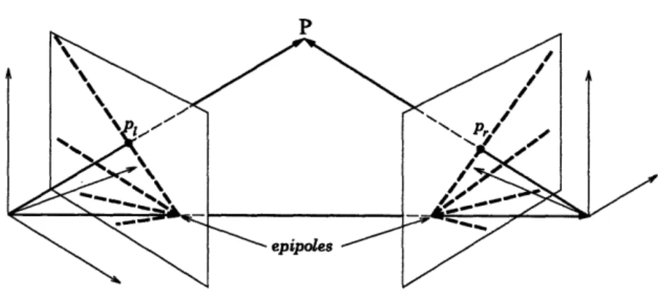
2.1.2 The epipolar constraint

Suppose we have two images taken at two different camera positions, which we will refer to as right and left. Let p, and Pi denote the position vectors with respect to the right and left coordinate systems to a fixed point P in the environment, p, = (Xr, yr, Zr)T and P, = (Xe, Ye, Ze)T. Assuming a fixed environment so that rigid body motion is applicable, Pr and pi are related by

Pr = Rpl + b (2.4)

where R denotes an orthonormal rotation matrix, and b is the baseline vector connecting the origins of the two systems. A necessary condition for the vectors Pr and pl to intersect at P is that they be coplanar with the baseline, b, or equivalently, that the triple product

of the three vectors vanish

Pr* (b x Rpl) = 0 (2.5)

Given R, b, and the coordinates (xe, ye, f) of the point Pe, which is the projection of P in the left image, equation (2.5) defines a line in the right image upon which the corresponding point P, at (xr, y,, f) must lie. This line, known as the epipolar line, is the intersection of the image plane with the plane containing the point P and the baseline b. The position of P' on the epipolar line is determined by the depth, or z-coordinate, of P in the left camera system. To see this, define the variables q, 4, and € to represent the components of the rotated homogeneous vector R e

(~

(2.6)

Then equation (2.4) can be expressed in component form as

X,

)

b.

Yr = Z 7 + by (2.7)

The projection of P onto the right image is found from

X

=

f

= f

b(2.8)

Z, Z10

+

bz

and r = f = f + b (2.9)

Zr

Zto

+

b,

Pr' thus varies along the epipolar line between f(b,/bz, b,/bz) when Ze = 0 to f(ý/1, 7r//) when Ze = oo. The first point, known as the epipole, is independent of xt and yt, and is therefore common to all epipolar lines. By rewriting (2.4) as

Pi = RTPr + b' (2.10)

where b' = -RTb, a similar relation can be obtained for the coordinates of the point Pj, the projection of P onto the left image plane, in terms of Z, and the components of the rotated vector RT P. The geometry of the epipolar transformation is illustrated in Figure 2-2.

CHAPTER 2. METHODS FOR COMPUTING MOTION AND STRUCTURE

FIGURE 2-2: Epipolar geometry.

Binocular stereopsis is based on the fact that the depth of objects in the scene can be recovered from their projections in two images with a known relative orientation. From (2.8) and (2.9) it is easily seen that

fbx - b, r fby - bzy,

Or - fA OYr - fA

(2.11)

The quantity Oxr - fý is known as the horizontal disparity, dH, and the quantity OYr - frq

as the vertical disparity, dv. If R = I and b = (Ib1, 0, 0), then ( = zl/f, € = 1 and equation (2.11) reduces to the familiar parallel geometry case in which

flbl

zr = zJ = f JI

(2.12)

and for which the vertical disparity is necessarily zero.

2.2

Computing Motion by Matching Features

In this section, we will examine only those methods which compute motion from point correspondences. Although algorithms using higher level features, such as lines and planes have been proposed ([22], [23], [24], [25]), these usually require more than two views and also are not as practical for hardware implementation.

To compute camera motion, or relative orientation, we need to find the rotation and baseline vector that best describe the transformation between the right and left camera

systems. We assume that we have a set of N pairs, {(ri, Li)}, i = 1,..., N, where ri and £i are the position vectors of the points P,, and P[ which are projectively equivalent, in the right and left systems respectively, to the same world point P.

The fundamental equation for computing the coordinate transformation between the two camera systems is the coplanarity constraint given by equation (2.5). Since this equation is homogeneous, it can be written in terms of ri and £i as

r -(b

x

Rfe) = 0

(2.13)

Equation (2.13) is unaffected by the lengths of any of the vectors ri, li, or b. We usually set hIb = 1 so that the baseline length becomes the unit of measure for all distances in the scene. The vectors ri and i£ may be set equal to the homogeneous vectors p,i and Pt

ri = ri and, L£ = • (2.14)

or may also be assigned unit length:

ri Prand, Li- P

(2.15)

IPTiI

Ipii

The second choice is often referred to as spherical projection.

2.2.1 Representing rotation

There are several ways to represent rotation, including orthonormal matrices as in (2.13). The matrix form is not always the best choice, however, as it requires nine coefficients, even though there are only three degrees of freedom. A rotation is completely specified by the pair (0,

W),

where 0 represents the angle of rotation about the axis W = (wX, wy, Wz)T, with

1W1

= 1. The relation between the orthonormal matrix R and (0,') is given by

cos 0 + w2(1 - cos 0) w,w (1 - cos 0) -w, sin 0 W,w (1 - cos 0) + wy sin 0

= ww, (1 - cos 0)

+

w, sin 0 cos O + W, (1 - cos 0) wyw (1 - cos 0) - w, sin 0 Vw,w(1 - cos 0) - w~ sin0

wvW,(1

- cos 0) + w. sin0 cos 0 +

w2(1

- cos 0)

(2.16)

which can also be expressed as

CHAPTER 2. METHODS FOR COMPUTING MOTION AND STRUCTURE

31

where

x

=

W , 0 - W, (2.18)

Equation (2.17) leads directly to Rodrigues' well-known formula for the rotation of a vector

R£ = cos Oe

+

(1 -cos 0)(. -)L

+

sin Ox I

= £+ sin _{O8 x £ + (1 - cos O)cO x (W x}

_x)

_(2.19) A frequently useful and compact representation of rotation is the unit quaternion. Quaternions are vectors in R4 _{which may be thought of as the composition of a scalar}

and 'vector' part [4].

a = (ao, a) (2.20)

where a = (a., ay, az)T is a vector in R3. An ordinary vector v in R3 _{is represented in}

quaternion form as

= (0, v) (2.21)

A unit quaternion is one whose magnitude, defined as the square root of its dot product with itself, is unity.

4 4 q = 1 (2.22)

Unlike vectors in R3, quaternions are endowed with special operations of multiplication and conjugation, and thus form the basis of a complete algebra. The fundamental operations and identities of quaternion algebra are summarized in Appendix A.

The usefulness of quaternions lies in the simplicity with which rotation about an arbi-trary axis can be represented. Every unit quaternion may be written as

=

cos , sin 2

(2.23)

and the rotation of the vector v by an angle 0 about W' by q'

where q* represents the conjugate of 4.

In the following discussions I will alternate between these different representations, to use whichever form is best suited to the problem at hand.

2.2.2 Exact solution of the motion equations

There are five unknown parameters in equation (2.13), two for the direction of the baseline and three for the rotation. It has long been known that relative orientation can be determined from a minimum of five points, as long as these do not lie on a degenerate surface. Due to the rotational component, however, the equations are nonlinear and must be solved by iterative methods. Furthermore, the five-point formulation admits multiple solutions' [7], [4].

Thompson [26] first showed how the coplanarity conditions could be formulated as a set of nine homogeneous linear equations, and Longuet-Higgins [27] proposed an algorithm to

derive the baseline vector and rotation matrix from the solution to the equations obtained from eight point correspondences. This algorithm is summarized as follows:

The first step is to rewrite the coplanarity constraint (2.13) as

ri (b x Ri)

= -R

(b x r)

= -ITRTBxri

(2.25)

where

S0

-be

by

B =

b

0

-bI,

(2.26)

-by

b

0O

We define the matrix E as

E = RTBx (2.27)

'Faugeras and Maybank [7] first proved that there are at most 10 solutions for the camera motion given 5 correspondences, thereby correcting a longstanding error by Kruppa [5] who had thought there were at most 11.

CHAPTER 2. METHODS FOR COMPUTING MOTION AND STRUCTURE

and order the components of E as

e7

e8

e9

(2.28)

Let aj denote the 9x1 vector formed from the products of the components of ri and

ei

rxi~xi rxieyi rxitzi ryieci

r,ifLi

ryifyi ryilzi rzi£xi rzilzi

and let e denote the 9x 1 vector of the elements of E. each pair of rays results in an equation of the form

(2.29)

Then the coplanarity constraint for

aiTe = 0

(2.30)

Eight correspondences result in eight equations which can be solved to within a scale fac-tor for the elements of E. Given E, the baseline vecfac-tor is identified as the eigenvecfac-tor corresponding to the zero eigenvalue of ETE

ETEb = 0 (2.31)

as can be seen from the fact that

ETE = BxTBx

The rotation matrix R is found from

R = BxET - Cof(ET)T (2.33)

where Cof(ET) is the matrix of cofactors of ET.

2.2.3 Least-squares methods

If there is no error in the data, the Longuet-Higgins algorithm will give a unique solution for the motion2 except for certain configurations of points which lie on special surfaces [8], [28]. It is extremely difficult, however, to obtain error-free data, particularly if the corre-spondences are determined by an automatic procedure. It turns out that the 8-point linear algorithm is extremely unstable in the presence of noise, due largely to the fact that the equations (2.30) do not take into account dependencies between the elements of E, and hence their solution cannot be decomposed into the product form of equation (2.27).

Even when nonlinear methods are used to solve the coplanarity constraint equations, the solution is very sensitive to noise when few correspondences are used [29]. With error in the data, the ray pairs are not exactly coplanar and equation (2.13) should be written as

Ri - (ri x b) = Ai (2.34)

Instead of trying to solve the constraint equations exactly, it is better to find the solution that minimizes the error norm

N

s =

A?

(2.35)

i=1

A somewhat improved approach over the 8-point algorithm was proposed by Weng et al. [30] based on a modification of a method originally presented by Tsai and Huang [28].

2

There is an intrinsic fourfold ambiguity to every solution; however, these are all counted as one. This ambiguity will be discussed in more detail in Chapter 7.

CHAPTER 2. METHODS FOR COMPUTING MOTION AND STRUCTURE

35

They defined an N x 9 matrix A as

aT\

T

A =

.2

(2.36)

alNI

such that S =

jAe

2'. The vector e which minimizes S is the eigenvector of ATA with the smallest eigenvalue. The baseline direction and rotation are derived from the resulting matrix E such that b minimizes IETEbl and R is the orthonormal rotation matrix that minimizes

IE

- RTB x 1

This method, however, also neglects the dependencies between the elements of E, and consequently is still very sensitive to errors in the data. The matrix formed from the elements of the vector e that minimizes |Ael is not necessarily close to the product of the matrices R and B x which correspond to the true motion.

Several researchers have pointed out the problems of computing motion by unconstrained minimization of the error [12], [3]. Horn [3] proposed the most general algorithm to solve the direct nonlinear constrained optimization problem iteratively. This method was later revised and reformulated in [4] using unit quaternions.

The vectors ri, £i, and b are given in quaternion form by

i = (0, r), ii = (0, ), and, = (0, b) (2.37) while that of i'i = Rfi is given by

'i = q i

4*

(2.38)

Using the identity (A.10) given in Appendix A, the triple product A₁ (2.34) can be written as

xi = rib

q 4i 4*

=

-qfi

(2.39)

In the latter version of Horn's algorithm, S, the sum of squared errors, is written as a first order perturbation about a given d and

4.

The idea is to find the incremental changes bS and Sq which minimize the linearized equation subject to the constraints

4~ = 1, a.d =, and, q d=0 (2.40)

The updated vectors q4 + 64 and d + ba must also satisfy these conditions and, neglecting second order terms, this results in the incremental constraints

S84

= 0, d6 = 0, and, -6d

+

d

= 0

(2.41)

Differentiating the constrained objective function with respect to 6S,

6d,

and the Lagrange multipliers A, /u, v associated with each of the constraints (2.41) and setting the result to zero results in a linear system of equations of the form

S A =h

(2.42)

where the matrix J and the vector h are both known, given the current value of

4

and d (see [4] for details). Equation (2.42) can thus be solved for the 11 unknowns, which are the four components each of 64 and 6d and the three Lagrange multipliers. After updating 4 and

a

with the new increments 64 and 6•, the procedure can be repeated until the percentage change in the total error falls below some limit. This algorithm has been shown to be very accurate and efficient in most cases for estimating motion, even with noisy correspondence data, as long as there are a sufficiently large number of matches. As presented, however, it is too complex to be implemented efficiently on a simple processor, given the need to solve an 11x 11 system of equations at each iteration. We will present a simplified adaptation of this algorithm in Chapter 7.

CHAPTER 2. METHODS FOR COMPUTING MOTION AND STRUCTURE

37

2.3

Correspondenceless Methods

If the displacements in the image are small, they can be approximated by the time derivatives of the position vectors to points in the scene. For small 0, cos 08 1, sin 0 , 0, and equation (2.17) reduces to

R ;, I + Oflx (2.43)

The equation of rigid body motion (2.4) then becomes Pr = RpI+b

= Pi + 0( x P) + b (2.44)

Let p denote the time derivative of the vector p, which can be approximated as p = p - p,. From (2.44)

p

= -O(W x p) - b (2.45)

which, expanded into component form, results in

(

((wY

- wZ)

-

b,

S

= o(w,Z - wX) - by

(2.46)

1

O(wc.Y - woX) - bz

Image plane displacements are given by

dx dy

U= d-

dt

xt- 2., and, v- dt -

dt

y-r (2.47) From the equations of perspective projection (2.1) we have

dzx d f _X\ X\

-dx fd =(X)= I _{X )Z (2.48)}

tdT

d Z Z Z

t

and

dy

f

(f-Y

Z _(2.49)

Combining (2.46) through (2.49), we obtain the equations for the incremental optical flow

S

-=fb

+ bzx +-0 (

-

w,(zX

+ f)

+•zy f)

(2.50)

=

-fb,

+

bzy

-

(wy-w(y

+

f2)

+

_Sf)

_(2.51)

first derived by Longuet-Higgins and Prazdny [31].

If it is assumed that the brightness E of a point in the image does not change as the point moves, then the total derivative of brightness with time must be zero, that is,

dE OE dx OE dy OE

0 + +

dt Ox dt Oy dt Ot

= Eu + Eyv + Et (2.52)

Equation (2.52) is known as the brightness change constraint equation.

There are two approaches to using these equations. The first, and earliest proposed, is to compute the optical flow over the entire image and to invert (2.50) and (2.51) to find the global motion and depth at each pixel. The second, known as the direct approach, skips the computation of the optical flow and uses only the constant brightness assumption combined with the incremental rigid body equations. Neither approach requires finding explicit point correspondences.

2.3.1

Optical flow

Horn and Schunck developed the first algorithm for determining optical flow from local image brightness derivatives [32] based on minimizing the error in the brightness change constraint equation

Eb = E.u + Eyv + Et (2.53)

Since there are two unknowns at each pixel, the constant brightness assumption is not sufficient to determine u and v uniquely and a second constraint is required. Horn and Schunck chose the smoothness of the optical flow and added a second error term

S=

IVU1

2

₊

_IV

V

_I

2

_(2.54)

The total error to be minimized is therefore

b

CHAPTER 2. METHODS FOR COMPUTING MOTION AND STRUCTURE

where A2 is a penalty term that weights the relative importance of the two constraints. The functions u and v which minimize Ec2 for a given A can be found using the calculus of variations.

One problem with computing optical flow by applying a smoothness constraint is that the flow is not smooth at boundaries between objects at different depths. The global optimization procedure causes errors generated at depth discontinuities to propagate to neighboring regions [33]. Segmenting the optical flow at depth discontinuities would appear to be the solution to this problem except that one does not know a priori where they are. Murray and Buxton [34] proposed incorporating discontinuities by adding line processes to the objective function, using an idea originated by Geman and Geman for segmenting gray-scale images by simulated annealing [35]. The resulting optimization problem is non-convex, however, and requires special procedures to converge to a global minimum energy state.

Once the optical flow is determined it is necessary to solve equations (2.50) and (2.51) to find motion and depth. As was the case for the explicit methods, absolute distances cannot be recovered since scaling Z and b by the same factor has no effect on u and v. Longuet-Higgins and Prazdny [31] showed how motion and depth parameters could be determined from the first and second derivatives of the optical flow after first computing the location of the epipole. Heeger et al. [36] proposed a method to recover the motion by applying rotation insensitive center-surround operators that allow the translational and rotational components of the motion to be determined separately. Ambiguities in interpreting the optical flow in the case of special surfaces have been analyzed in [37], [38], [39], and [40].

2.3.2 Direct methods

The method of Horn and Schunck, or one of its variations, requires a great deal of computation to determine the optical flow-which is only an intermediate step in obtain-ing the actual parameters of interest. The direct approach of Horn and Weldon [41] and Negahdaripour and Horn [42] avoids computing optical flow by substituting u and v from equations (2.50) and (2.51) directly into (2.52). The brightness change constraint equation is thus expressed as

s-b

where

s=

- fE1

(2.57)

and

fE, + y(xE, + yE,)/f

v = -fE

-

z(xE. + yE)/lf

(2.58)

yE, - zEy

Note that the vectors s and v are entirely computable from measurements in the image. Assuming the image contains N pixels, there are N + 5 unknowns in equation (2.56): the five independent parameters of b and

Z06

(recall that b is a unit vector due to the scale factor ambiguity), and the N depth values Z. Since there is only one equation (2.56) for each pixel, the problem is mildly underconstrained. Given two images it can be solved only for a few special cases in which either the motion or the surface structure is restricted. With more than two views of the same scene, however, the problem is no longer underconstrained [11]. It should be noted that it is never required to incorporate the assumption that the optical flow is smooth, and hence the problems associated with discontinuities in the flow are avoided.

Several methods have been developed to solve the special cases where the problem is not underconstrained for two views. Three of these were developed by Negahdaripour and Horn who gave a closed form solution for motion with respect to a planar surface [43]; showed how the constraint that depth must be positive could be used to recover translational motion when the rotation is zero, or is known [44]; and derived a method for locating the focus of expansion [45]. Taalebinezhaad [46], [47] showed how motion and depth could be determined in the general case by fixating on a single point in the image. He essentially demonstrated that obtaining one point correspondence would provide enough information to enable the general problem to be solved.

2.3.3

Limitations of correspondenceless methods

Methods for computing motion and depth from the local spatio-temporal derivatives of image brightness must rely on specific assumptions in order to work. The most impor-tant of these, on which all of the methods just described are based, is that brightness is

CHAPTER 2. METHODS FOR COMPUTING MOTION AND STRUCTURE

constant (2.52). Verri and Poggio [48] criticized differential methods on the grounds that brightness constancy is often violated. Their arguments, however, were based on consid-ering shading effects which are important only for specular surfaces or when the motion is large enough to significantly affect surface orientation. Furthermore, these effects domi-nate only when the magnitude of the spatial brightness gradient is small. There are clearly cases, such as the rotating uniform sphere or the moving point light source, as pointed out by Horn [49] and others, in which the optical flow and the motion field are different. In areas of the image where the brightness derivatives are small, it is difficult to constrain the motion or to determine depth. However, this problem is not specific to differential methods. Gennert and Negahdaripour [50] investigated the use of a linear transformation model to account for brightness changes due to shading effects on lightly textured surfaces. Their method was applied only to computing optical flow and involved modifying the objective function (2.55) to add new constraints. Direct methods do not lend themselves as easily to relaxing the brightness constancy assumption. With these it is simpler to ignore areas where the spatial derivatives are small.

One of the more important assumptions underlying differential methods is that the interframe motion must be small so that the approximations (2.43)-(2.45) will be valid, and so that the spatial and temporal sampling rates will not violate the Nyquist criterion. It is useful to perform some sample calculations to see what is meant by "small". The approximations sin 0 - 0, cos 0

8

1 are accurate to within 1.5% to about 100 of rotation. Approximations (2.45) and (2.47) which express the derivatives of the position vector as the difference between the left and right rays, and which incorporate the approximation R I + Oflx, are thus reasonable as long as the velocity of the point in the scene is constant between frames and 0 < 100. These conditions should not be difficult to achieve with video-rate motion sequences. The angular restriction may rule out some binocular stereo arrangements, however.

The primary concern is thus not the validity of the incremental optical flow equations, but whether the sampling rates are high enough to avoid aliasing. The Nyquist criterion which bounds the maximum rate at which an image sequence can be sampled in space and time can be derived as follows.

The constant brightness assumption requires that