HAL Id: hal-00481732
https://hal.archives-ouvertes.fr/hal-00481732
Submitted on 10 May 2021
HAL is a multi-disciplinary open access
archive for the deposit and dissemination of
sci-entific research documents, whether they are
pub-lished or not. The documents may come from
teaching and research institutions in France or
abroad, or from public or private research centers.
L’archive ouverte pluridisciplinaire HAL, est
destinée au dépôt et à la diffusion de documents
scientifiques de niveau recherche, publiés ou non,
émanant des établissements d’enseignement et de
recherche français ou étrangers, des laboratoires
publics ou privés.
Distributed under a Creative Commons Attribution| 4.0 International License
finmarchicus and C. helgolandicus in the North Atlantic
Ocean and adjacent seas.
P. Helaouet, Gregory Beaugrand
To cite this version:
P. Helaouet, Gregory Beaugrand. Macro-ecological study of the niche of Calanus finmarchicus and C.
helgolandicus in the North Atlantic Ocean and adjacent seas.. Marine Ecology Progress Series, Inter
Research, 2007, pp.147-165. �hal-00481732�
INTRODUCTION
Understanding the consequences of variability in cli-mate on pelagic ecosystems requires a clear identifica-tion of the factors driving variability in the abundance of each species and the parameters or processes that control their geographical distribution. Biogeographi-cal studies are essential and provide a baseline for
evaluation of the impact of climate on ecosystems (Longhurst 1998, Beaugrand 2003).
The high nutrient supply in the temperate and sub-polar part of the North Atlantic Ocean results in high planktonic production (Ducklow & Harris 1993, Long-hurst 1998). This region is influenced by the North Atlantic Current which transfers energy and heat from the SW oceanic region of Newfoundland to the NE
© Inter-Research 2007 · www.int-res.com *Email: [email protected]
Macroecology of
Calanus finmarchicus and
C. helgolandicus in the North Atlantic Ocean
and adjacent seas
Pierre Helaouët
1, 2,*, Grégory Beaugrand
11Centre National de la Recherche Scientifique (CNRS), FRE 2816 ELICO, Station Marine, BP 80, 62930 Wimereux, France 2
Present address: Sir Alister Hardy Foundation for Ocean Science, The Laboratory, Citadel Hill, Plymouth PL1 2PB, UK
ABSTRACT: Global climate change is expected to modify the spatial distribution of marine organ-isms. However, projections of future changes should be based on robust information on the ecologi-cal niche of species. This paper presents a macroecologiecologi-cal study of the environmental tolerance and ecological niche (sensu Hutchinson 1957, i.e. the field of tolerance of a species to the principal factors of its environment) of Calanus finmarchicus and C. helgolandicus in the North Atlantic Ocean and
adjacent seas. Biological data were collected by the Continuous Plankton Recorder (CPR) Survey, which samples plankton in the North Atlantic and adjacent seas at a standard depth of 7 m. Eleven parameters were chosen including bathymetry, temperature, salinity, nutrients, mixed-layer depth and an index of turbulence compiled from wind data and chlorophyll a concentrations (used herein
as an index of available food). The environmental window and the optimum level were determined for both species and for each abiotic factor and chlorophyll concentration. The most important para-meters that influenced abundance and spatial distribution were temperature and its correlates such as oxygen and nutrients. Bathymetry and other water-column-related parameters also played an important role. The ecological niche of C. finmarchicus was larger than that of C. helgolandicus and
both niches were significantly separated. Our results have important implications in the context of global climate change. As temperature (and to some extent stratification) is predicted to continue to rise in the North Atlantic sector, changes in the spatial distribution of these 2 Calanus species can be
expected. Application of this approach to the 1980s North Sea regime shift provides evidence that changes in sea temperature alone could have triggered the substantial and rapid changes identified in the dynamic regimes of these ecosystems. C. finmarchicus appears to be a good indicator of the
Atlantic Polar Biome (mainly the Atlantic Subarctic and Arctic provinces) while C. helgolandicus is
an indicator of more temperate waters (Atlantic Westerly Winds Biome) in regions characterised by more pronounced spatial changes in bathymetry.
KEY WORDS: Macroecological approach · Hutchinson ecological niche · Biogeography · Calanus finmarchicus · Calanus helgolandicus · North Atlantic Ocean · Continuous Plankton Recorder
part of the North Atlantic Ocean (Krauss 1986). This current also has a profound impact on plankton diver-sity (Beaugrand et al. 2001). The North Atlantic Ocean is divided into 3 biomes: the Atlantic Polar Biome, the Atlantic Westerly Winds Biome and the Atlantic Coastal Biome, each divided into a number of pro-vinces (present Fig. 1; Longhurst 1998). Their ecological characteristics have been recently reviewed by Long-hurst (1998) and some complementary descriptions have been added by Beaugrand et al. (2001, 2002) for the northern part of the North Atlantic Ocean and its adjacent seas.
Copepods constitute a key trophic group, with a cen-tral role in the trophodynamics of pelagic ecosystems. These plankton organisms transfer energy from the phytoplankton to higher trophic levels (Mauchline 1998) and are often important in the diet of at least 1 developmental stage of economically important fish species such as cod, herring or mackerel (Sundby 2000, Orlova et al. 2005, Skreslet et al. 2005). Cope-pods represent a high proportion of the carbon bio-mass in the mesozooplankton, generally increasing with increasing latitude (e.g. 33% for the Atlantic Trade Wind Biome, 53% for the Atlantic Westerly Winds Biome and 69% for the Arctic Ocean, Longhurst 1998). Members of the genus Calanus are amongst the
largest copepods and can comprise as much as 90% of the dry weight of the mesozooplankton in regions such as the North Sea and the Celtic Sea (Bonnet et al. 2005 and references therein). The congeneric calanoid copepod species C. finmarchicus and C. helgolandicus
have been well studied (e.g. Planque & Fromentin 1996, Bonnet et al. 2005). They are morphologically so similar that they were not distinguished until 1958, in the Continuous Plankton Recorder (CPR) survey (Planque & Fromentin 1996). However, their spatial distribution differs significantly (Beaugrand 2004a). C. finmarchicus is mainly located in the Atlantic Polar
Biome north of the Oceanic Polar Front (Dietrich 1964, Beaugrand 2004a; present Fig. 1) while the pseudo-oceanic species C. helgolandicus occurs in more
tem-perate waters south of the Oceanic Polar Front, mostly located above the European shelf-edge in the Atlantic between 40 and 60° N (Beaugrand 2004a, Bonnet et al. 2005). In regions where they occur together (e.g. the North Sea), the 2 species generally have different sea-sonal timing (Beaugrand 2003). Some studies have also reported different depth of occurrence at the same location (Bonnet et al. 2005 and references therein).
Differences in the spatial and/or temporal patterns of variability in both species ofCalanus suggest
differen-tial responses to environmental variability. It is there-fore important to identify their environmental prefer-ence (window or tolerance interval) and their optimum environmental level. When the preference of more than 1 factor has been determined, the ecological niche (sensu Hutchinson 1957) can be calculated (i.e. the field of tolerance of a species to the principal fac-tors characteristic of its environment). The niche can be represented in Euclidean space with as many dimensions as factors considered. When a few num-bers of parameters are used, the niche of 2 species may overlap. Increasing the number of factors reduces the relative importance of such overlap and often enables complete niche separation (Gause’s competitive ex-clusion hypothesis: Gause 1934). Abiotic parameters are related to both geographic (e.g. topography) and water-column (e.g. nutrient concentration) factors which influence directly the physiology (e.g. growth, development and mortality rates, Carlotti et al. 1993) or reproduction (Hall & Burns 2002, Halsband-Lenk et al. 2002) of a species. This study investigated abiotic environment and chlorophyll a concentration (as an
index of available food), for which the Hutchinson eco-logical niche is a more suitable tool, often preferred in this type of work (e.g. Pulliam 2000, Guisan & Wilfried 2005).
Despite the large number of studies on the biology and ecology of both Calanus finmarchicus and C. helgo-landicus (e.g. Carlotti et al. 1993, Hirst & Batten 1998,
Heath et al. 1999, Bonnet et al. 2005), many gaps in our knowledge remain. Herein we employ a macroecolog-ical approach using large data sets of 11 abiotic para-meters and data from the CPR survey to (1) determine the environmental optimum level of both species for each environmental parameter, (2) quantify the
influ-Fig. 1. Main area (light grey) sampled by the Continuous Plankton Recorder survey from 1960 to 2002, and provinces (Longhurst 1998). Atlantic Polar Biome — SARC: Atlantic sub-arctic province; ARCT: Atlantic sub-arctic province. Atlantic West-erly Winds Biome — NADR: North Atlantic Drift province; NAST: North Atlantic subtropical gyral province (W and E: western and eastern parts, respectively); GFST: Gulf Stream province. Atlantic Coastal Biome — NECS: Northeast Atlantic shelves province; NWCS: Northwest Atlantic shelves province.
ence of each parameter on both species, (3) identify and (4) calculate the breadth of their ecological niches. The temporal stability of the temperature profiles of both species is also investigated. A baseline is pro-vided for use in forecasting modifications in the abun-dance and spatial distributions of the 2 species that can be expected with global climate change.
MATERIALS AND METHODS
Biological data. Data on the abundance of Calanus finmarchicus and C. helgolandicus were provided by
the CPR survey, a large-scale plankton monitoring pro-gramme initiated by Sir Alister Hardy in 1931. The CPR is a robust instrument designed for use by seamen on commercial ships. Management and maintenance of the survey have been carried out by the English lab-oratory (Sir Alister Hardy Foundation for Ocean Sci-ence [SAHFOS]) since 1990. CPR instruments are towed at a depth of 7 m (Reid et al. 2003a) and the sur-vey has monitored plankton ecosystems at this depth only (Batten et al. 2003). Therefore, it might be danger-ous to infer Hutchinson’s ecological niche from a single depth. However, calanoid copepods migrate vertically (Daro 1985) and because CPR sampling is carried out both day and night, it is unlikely that this process greatly influenced the measurement of the Hutchinson ecological niche in this study.
Water enters the CPR through an inlet aperture of 1.61 cm2 and passes through a 270 μm silk-covered
filtering mesh (Batten et al. 2003). Individuals > 2 mm, such as Copepodite Stages CV and CVI ofCalanus fin-marchicus and C. helgolandicus are then removed
from the filter and covering silk. Generally, all individ-uals are counted, but for particularly dense samples a sub sample is taken (Batten et al. 2003). The data used in this study correspond to Copepodite Stages CV and CVI. Studies have shown that near surface sampling provides a satisfactory representation of the epipelagic zone (Batten et al. 2003). This programme has accumu-late one of the greatest databases on marine plankton worldwide. Currently, about 200 000 samples have been analysed, providing information on the presence and/or abundance of more than 400 plankton species every month since 1946 in both the temperate and sub-polar region of the North Atlantic Ocean.
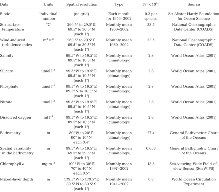
Environmental data. We investigated the area from Longitude 99.5° W to 19.5° E and Latitude 29.5° to 69.5° N. Eleven parameters were chosen (Table 1). Sea surface temperature (SST) was essential as it has a well-documented effect on plankton (e.g. Reid & Edwards 2001). Wind-induced water turbulence was used as an indicator because it has been shown that wind, by its impact on water-column stability, affects
plankton populations (Heath et al. 1999). The index of turbulence and SST was aquired from the Comprehen-sive Ocean-Atmosphere Data Set (COADS) and was downloaded from the internet site of the National Oceanographic Data Center (NODC) (Woodruff et al. 1987), which manages acquisition, controls quality and safeguards the data.
Salinity also constitutes an important limiting factor for many species. Data on this parameter, and on sili-cates, phosphates, nitrates and dissolved oxygen were downloaded from the World Ocean Atlas 2001 (WOA1) database for a depth of 10 m.
Bathymetry was selected because it has been sug-gested that this parameter influences the distribution of some copepod species (Beaugrand et al. 2001). Bathymetry data originate from the database ‘General Bathymetric Chart of the Oceans’ (GEBCO). Spatial variability in bathymetry was assessed over the study area. First, the mean and SD of bathymetry data were calculated in a geographical cell of 1° latitude and 1° longitude, (225 data per geographical cell). Then, the coefficient of variation of bathymetry (CVB) was
calcu-lated as:
(1) where mBis the average and SBthe SD for bathymetry
in each geographical cell. There was generally high variability in bathymetry over the continental slope regions.
Chlorophyll is a potentially influential parameter because the 2 selected species are mainly herbivorous (Mauchline 1998). However as Kleppel (1993) showed and Mauchline (1998) stressed, the dietary require-ments of copepods change from the first nauplii stage to the adult stage and are likely to vary at both diel and seasonal scales. Furthermore, it is likely that bothCalanus species also feed on microzooplankton
(Mauchline 1998). Therefore, chlorophyll content should only be considered as an index of food avail-ability. Chlorophyll values originated from the pro-gramme ‘Sea-viewing Wide Field-of-view Sensor’ (SeaWIFS) from the National Aeronautics and Space Administration (NASA).
The mixed-layer depth (MLD) is another indicator of water column stability. In contrast to the index of turbulence, this parameter is obtained from vertical profiles of temperature and salinity. MLD data come from a compilation of about 4.5 million profiles gath-ered by the NODC and World Ocean Circulation Experiment (WOCE). These profiles are the result of the analysis of data from 1941 to 2002 and originate from various measuring instruments such as the conductivity-temperature-depth (CTD) monitor, mech-anical bathythermograph (MBT) or expendable bathy-thermograph (XBT).
CVB B
B
= S
Pre-processing of data. The first stage of the analy-sis conanaly-sisted of homogenising both environmental and biological variables. All original data tables were converted into 3 types of matrix: (1) matrices (2.48 million data points) with data for each month and year for the period 1960 to 2002 (temperature, wind stress); (2) matrices (57 600 data points) with data for each month (nutrients, oxygen, chlorophyll, MLD) based on the average of time periods ranging from 5 to 43 yr; (3) matrices (4800 data points) with no infor-mation on time (bathymetry and its spatial variability). The 3 types of environmental grids were used to re-gularise biological data, and no spatial interpolation was made. An arithmetic mean was calculated when the number of data for a given location and time period was >1.
Statistical analyses. Fig. 2 summarises the different statistical analyses performed in this study.
Analysis 1 — Characterisation of environmental optima at seasonal scale: The optimum of each species
was identified for each environmental variable (a total of 22 environmental profiles: 2 species × 11 environ-mental parameters). A profile was a contour diagram of a matrix of 12 mo × n environmental categories. To determine the number of environmental categories, the minimum and maximum values were first calcu-lated. Then, intervals were chosen by trial and error as a compromise between the resolution of the profile and the increasing number of missing data with increasing resolution. The profile matrix was assessed by aver-aging abundance data for each month and environ-mental category. Abundance data were
log-trans-Data Units Spatial resolution Type N (× 106) Source
Biotic Individual (no grid) Each month 0.2 per Sir Alister Hardy Foundation
number for 1946–2002 species for Ocean Science
Sea surface °C 260.5° to 29.5° E Monthly mean 33.5 National Oceanographic
temperature 69.5° to 30.5° N 1960–2002 Data Center (COADS)
(each 1°)
Wind-induced m3s– 3 260.5° to 29.5° E Monthly mean 33.5 National Oceanographic
turbulence index 69.5° to 30.5° N 1960–2002 Data Center (COADS)
(each 1°)
Salinity 99.5° W to 19.5° E Monthly mean 2.8 World Ocean Atlas (2001)
89.5° to 10.5° N (climatology) (each 1°)
Silicate μmol l–1 99.5° W to 19.5° E Monthly mean 2.8 World Ocean Atlas (2001)
89.5° to 10.5° N (climatology) (each 1°)
Phosphate μmol l–1 99.5° W to 19.5° E Monthly mean 2.8 World Ocean Atlas (2001)
89.5° N to 10.5° N (climatology) (each 1°)
Nitrate μmol l–1 99.5° W to 19.5° E Monthly mean 2.8 World Ocean Atlas (2001)
89.5° to 10.5° N (climatology) (each 1°)
Dissolved oxygen ml l–1 99.5° W to 19.5° E Monthly mean 2.8 World Ocean Atlas (2001)
89.5° to 10.5° N (climatology) (each 1°)
Bathymetry m 80° W to 20° E Monthly mean 27.4 General Bathymetric Chart
90° to 10° N (climatology) of the Oceans
each 0.4°
Spatial variability m 99.5° W to 19.5° E Monthly mean 0.058 General Bathymetric Chart
in the bathymetry 69.5° to 29.5° N (climatology) of the Oceans
(each 1°)
Chlorophyll a mg m– 3 100° W to 30° E Monthly mean 18.8 Sea-viewing Wide
Field-of-70° to 40° N 1997–2002 view Sensor (SeaWIFS)
each 0.5°
Mixed-layer depth m 179.5° W to 179.5° E Monthly mean 0.8 World Ocean Circulation
89.5° N to 89.5° S 1941–2002 Experiment
(each 1°)
formed (log10[x+1]) to limit the effect of extreme
values.
Analysis 2 — Quantification of importance of each environmental parameter at seasonal scale: A
princi-pal components analysis (PCA) was used to quantify the influence of each abiotic factor and chlorophyll concentration (used herein as an index of available food) on spatial and seasonal changes in Calanus spp.
abundance at the scale of the North Atlantic Ocean (Fig. 2). An algorithm that took into consideration miss-ing data was used to calculate the eigenvectors (Bou-vier 1977). This method of ordination made possible a summary of multivariate information in a reduced number of dimensions, i.e. the principal components (Jolliffe 1986). The normalised eigenvectors allowed identification of the variables contributing most to the principal components. The PCA was calculated from (120 longitudes × 40 latitudes × 12 mo) × 11 environ-mental variables. The spatial grid had a resolution of 1° longitude and 1° latitude. This table was centred and reduced prior to application of the analysis to remove any effect of scale between environmental variables.
Analysis 3 — Identification of ecological niche at seasonal scale: To identify the ecological niche of both
species, we used the first 3 principal components. The concept of ecological niche used in this study is that of Hutchinson (1957) which states that the niche is the field of tolerance of a species to the principal factors of its environment. The concept has been refined here by the recent improvements discussed by Frontier et al. (2004). In particular, our analysis takes into account that some factors are not independent but covary either pos-itively or negatively. The use of principal components decreases the effect of multicollinearity in the data (Le-gendre & Le(Le-gendre 1998). We repeated the procedure used in Analysis 1 to map the ecological niche of both
Calanus species as a function of principal components
(linear combination of environmental factors).
Analysis 4 — Quantification and comparison of Hutchinson’s niches: Quantification and comparison of
Hutchinson’s niche for both Calanus species were
per-formed for 4 different categories of abundance. The first category was based on all presence data: the value of the 11 environmental variables was retained when an individual (C. finmarchicus or C. helgolandicus) was
recorded in a geographical cell within the environmen-tal grid of 1 × 1° (Longitude 99.5° W to 19.5° E, Latitude 29.5° N to 69.5° N); a total of 24 subsets was determined (12 mo × 2 species). A similar procedure was applied to the other 3 categories. The second category comprised
Calanus spp. data greater than the first quartile, the
third category Calanus spp. data greater than the
me-dian and the fourth category data for Calanus spp.
greater than the third quartile. The breadth of the niche thereby decreased from Category 1 to Category 4. The
Fig. 2. Calanus finmarchicus and C. helgolandicus. Summary of statistical analyses performed in this study. PCA: principal component analysis; CPR: Continuous Plankton Recorder
quartiles and median were assessed from the biological data table in Fig. 2. There-fore, the quantification and comparison of Hutchinson’s niche for the 2 species used 96 (24 × 4) subsets.
To assess and compare Hutchinson’s niche for the 2 Calanus species, we used a
numerical analysis based on ‘multiple response permutation procedures’ (MRPP) and recently applied to determine the ecological niche by G. Beaugrand & P. Helaouët (unpubl. data). The method quantifies the breadth of the niche of the 2 species and tests if their niches are statis-tically different. First, quantification of the niche was made by calculating the mean Euclidean distance for each subset based on the 11 environmental parameters. The higher the mean Euclidean value, the greater Hutchinson’s niche. Second, for a given month and category, a weighted mean of the Euclidean distance of both species niche was calculated. Then, the weighted distance was tested by permuta-tions of original subset. A value of 10 000 permutations was selected. For each sim-ulation, the weighted distance was re-calculated and the probability that the separation of the niches of C. finmarchi-cus and C. helgolandifinmarchi-cus wouold be
sig-nificant was represented by the number of times the recalculated weighted distance was inferior to that observed.
Analysis 5 — Calanus thermal profiles as a function of state of North Atlantic Oscillation (NAO) and 1987 regime shift:
One important issue was to determine whether Hutchinson’s niche was constant at a decadal scale and whether it was in-fluenced by climate variability during the
period of investigation (1958 to 2002). In the latter case, the species should be able to acclimatise quickly to cli-mate change. To test this, we calculated the thermal profile of both species for negative NAO (NAO index <–1), medium NAO (–1 ≤ NAO index ≤ 1) and positive NAO (NAO index >1). Thermal profiles were calcu-lated according to a procedure identical to Analysis 1. To examine the potential impact of the regime shift in the North Sea (Beaugrand 2004b), thermal profiles were also assessed for years prior to and after 1987.
Analysis 6 — Calanus thermal profiles as a function of CPR data for daylight and dark periods. Changes in
the depth distribution of Calanus spp. through time
could bias our assessment of Hutchinson’s niche, as the CPR survey samples at a standard depth of about 7 m.
To evaluate if this process could have significantly affected ours results, we assessed the thermal profile (Analysis 1) of both species for CPR samples collected during daylight (CPR samples collected between 10:00 and 16:00 h) and dark (CPR samples collected between 22:00 and 04:00 h) (Beaugrand et al. 2001; their Fig. 1).
RESULTS
Spatial distribution of biological and environmental data
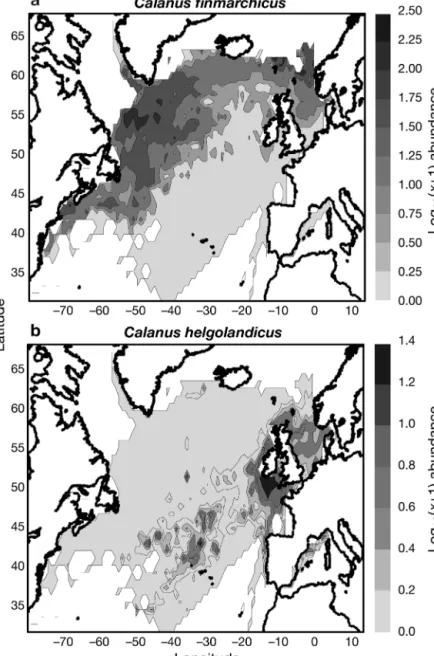
Fig. 3 shows the mean spatial distribution of Calanus finmarchicus and C. helgolandicus for the period 1958
Fig. 3. (a) Calanus finmarchicus and (b) C. helgolandicus. Spatial distribution in North Atlantic Ocean. No interpolation made
to 2002. The spatial distribution of C. finmarchicus
(Fig. 3a) was located north of the Oceanic Polar Front (Dietrich 1964) with 2 main centres of distribution south of the Labrador Sea and in oceanic regions south
and west of Norway (Fig. 3a). Fig. 3a suggests that this species is an indicator of the Atlantic Polar Biome and espe-cially the Atlantic Arctic Province and the Atlantic Subarctic Province as de-fined by Longhurst (1998). The spatial distribution of C. helgolandicus differed
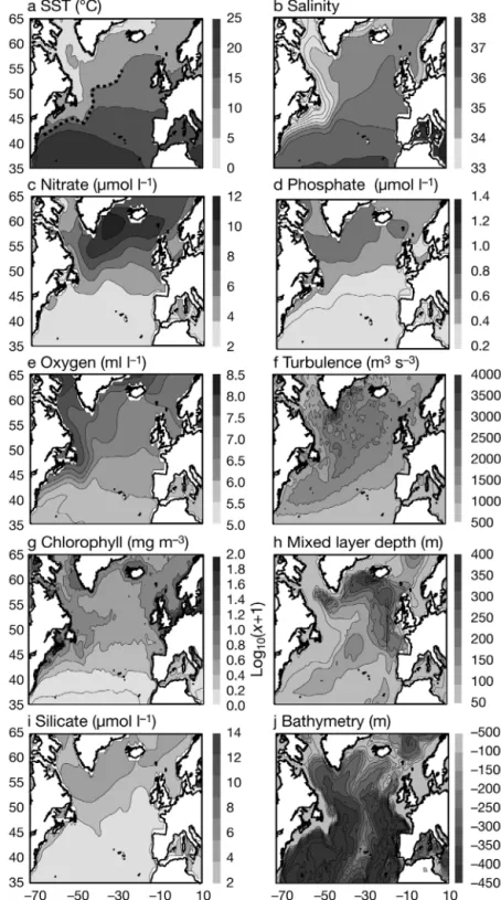
(Fig. 3b), being mainly centred along the shelf-edge in temperate regions. Fig. 4 presents the mean values of the environ-mental parameters in the North Atlantic Ocean. Temperature is an important driving mechanism for C. finmarchicus,
while it probably has a more limited role for C. helgolandicus (Fig. 4j).
Environmental profiles
Monthly thermal profile
Fig. 5 shows the thermal profile of
Calanus finmarchicus (Fig. 5a) and of C. helgolandicus (Fig. 5b) for each month. C. finmarchicus had its maximal
abun-dance between April and September at temperatures ranging from 6 to 10°C.
C. helgolandicus had a tolerance range
between 11 and 16°C, especially in spring (Fig. 5b). A remarkable feature was that the optimum varied seasonally-for both species. Each species had a clear distinct thermal optimum. The tolerance interval for C. finmarchicus was greater
than that of its congener. Fig. 5c shows the mean abundance of C. finmarchicus
and C. helgolandicus as a function of
temperature. The complementarity in the distribution of the 2 species is sig-nificant. The results show that a temper-ature change in a region with an annual thermal regime of about 10°C could trig-ger a shift from a system dominated by
C. finmarchicus to a system dominated
by C. helgolandicus.
Other profiles
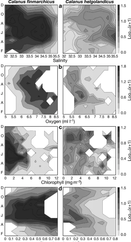
Fig. 6 presents further environmental profiles. Salinity profiles separated the 2
Calanus species well (Fig. 6a). C. finmarchicus had its
maximal abundance at salinities between 33.8 and 35 in the spring and summer months. The salinity opti-mum was higher for C. helgolandicus (35 to 35.5).
Dis-Fig. 4. Spatial distribution of (a) mean sea surface temperature (SST), (b) salin-ity, (c) nitrate, (d) phosphate, (e) dissolved oxygen, (f) turbulence, (g) chloro-phyll a, (h) mixed-layer depth, (i) silicate, (j) bathymetry. Location of the
solved oxygen content also distinguished the 2 species (Fig. 6b). Abundance of C. finmarchicus was maximal
at 6.4 to 7.3 ml l–1, C. helgolandicus was found in water
with less oxygen (5.9 to 6.6 ml l–1). Chlorophyll a
con-centration did not completely, separate the species (Fig. 6c). Nutrients were also examined. Fig. 6d shows an example of a profile for phosphate. Higher abun-dance of C. finmarchicus corresponded to phosphate
concentrations between 0.2 and 0.8 μmol l–1. For C.
helgolandicus, the optimum was between 0.1 and
0.3 μmol l–1. As in the case of salinity and temperature,
high abundance of C. helgolandicus
was located in a more restricted tol-erance range and time interval. Other nutrient profiles (nitrate and silicate; not shown) showed that
C. finmarchicus occured in waters
containing more nutrients than its congener. C. finmarchicus was
located in waters with a higher index of turbulence than C. helgo-landicus (data not shown). Similar
results were found for the mixed-layer depth (data not shown).
Calanus finmarchicus was mainly
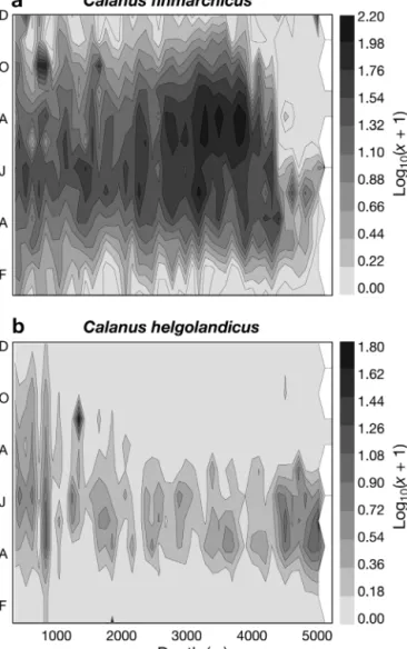
abundant at depths ranging from 269 to 3513 m, but can be found in regions of low bathymetry (Fig. 7a). The species was primarily found in regions with low to medium spatial variability in bathymetry. C. helgo-landicus was more often found in
regions characterised by a bathy-metry between 82 and 1216 m, despite the fact that a second mode was detected at depths > 4000 m (Fig. 7b). This last mode was proba-bly related to expatriate individuals in the region near the Bay of Biscay (see Fig. 3b). The species was iden-tified in regions characterised by a higher spatial variability in bathy-metry, reinforcing its classification as pseudo-oceanic (i.e. occurring in both neritic and oceanic regions but is mainly abundant above the shelf-edge).
Quantification of factors influencing spatial distribution
A PCA was calculated for each variable from 4800 12-mo geo-graphical squares × 11 variables. The first axis explained 42.3% of the total variance, the second 20.8%, the third 9.5% and the fourth 7.2%. The calculation of equiprobability (E):
where N is the number of variables, indicated that all
axes with a variance of more than 9.1% can be consid-ered significant. Therefore, only the first 3 normalised eigenvectors and principal components (representing 72.6% of the total variance) were retained. Fig. 8 pre-sents a scatterplot of the first 2 normalised eigenvectors
E N
=
( )
1 ×100Fig. 5. Calanus finmarchicus and C. helgolandicus. (a,b) Contour diagram of abun-dance (decimal logarithm) as a function of SST and month of year, and (c)
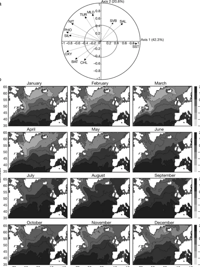
and maps of the first principal component. Variables such as temperature (relative contribution, RC = 82%); phosphate (RC = 75.1%), oxygen (RC = 73.8%), silicate (RC = 62.9%) and nitrate (RC = 54.7%) contributed greatly to the first component. Temperature was corre-lated negatively with the above factors (Fig. 8a).
Map-ping of the first principal component iden-tified a northward change from March to August and then a reverse movement from September to December (Fig. 8b). The Oceanic Polar Front (Dietrich 1964) was clearly identified (for location see Fig. 1). An asymmetry in the seasonal changes of the physical–chemical parameters was detected. The northern limit of the west-ern part of the Atlantic basin remained rel-atively constant at a monthly scale while in the eastern part the seasonal northward movement was much more pronounced. The influence of bathymetry on the first principal component was not detected.
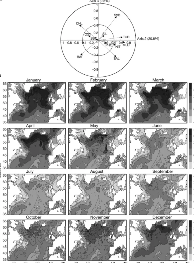
Fig. 9 is a scatterplot of the second and third normalised eigenvectors and maps of the seasonal changes in the second principal component at a seasonal scale. Variables that contributed mostly to the second principal component were mixed-layer depth (RC = 51.1%), index of turbu-lence (RC = 43.7%) and, to a lesser extent, chlorophyll concentration (RC = 27.1%), the index of spatial variability in metry (RC = 23.2%) and average bathy-metry (RC = 22.9%). Mapping of seasonal changes in the second principal compo-nent (Fig. 9b) showed the importance of parameters related to water-column struc-ture and the stable-biotope component (i.e. geographically stable, e.g. variables related to bathymetry). The effect of water-column structure was especially strong in the Atlantic Arctic Biome.
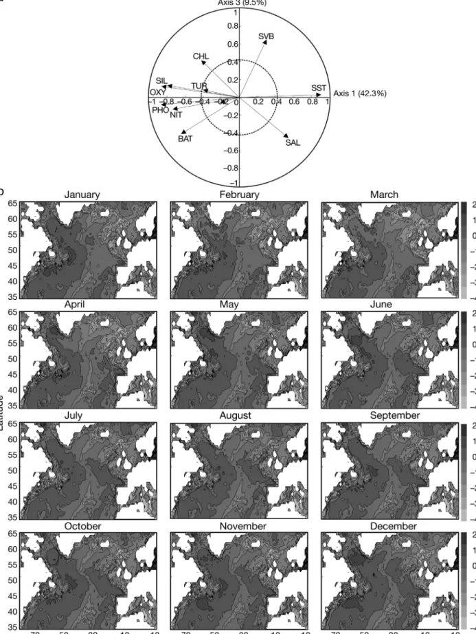
Fig. 10a shows that the main parameter related to the third principal component was primarily the index of spatial variabil-ity in bathymetry (RC = 42.4%) so that the third principal component (Fig 10b) directly highlighted the bathymetry of the region.
Identification of ecological niche
Using the first 3 principal components, a representation of the ecological niche (sensu Hutchinson 1957) is outlined in Fig. 11, which suggests that the ecological niche of both Calanus species is well separated. The
graphical was confirmed by the MRPP-based test, which indicated a statistically significant separation of the niche for each month and abundance category (Table 2). Quantification of the breadth of the niche fur-ther indicated that the niche breadth of C. finmarchicus
Fig. 6. Calanus finmarchicus and C. helgolandicus. Abundance (in decimal logarithm) as a function of month of year and of (a) salinity, (b) dissolved
was overall larger (e.g. niche breadth index = 8.2 for January) than that of its congener (e.g. niche breadth index = 7.4 for January) when the estimation was based on presence data, whatever the month. When higher categories of abundance were considered, few excep-tions were detected; these corresponded to the main seasonal maximum of the 2 species. These exceptions might be related to the positive relationship between dispersal and abundance of the 2 species.
Application of ecological niche approach to explain change in dominance
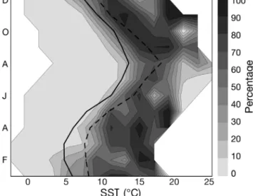
Temperature was the most important environmental parameter according to PCA results. This parameter sep-arated the 2 species well. Fig. 12 shows changes in the proportion of Calanus helgolandicus as % of total Calanus (C. finmarchicus and C. helgolandicus) as a
function of temperature. The location of the line below which 10% of Calanus identified by the CPR survey
were C. helgolandicus varied monthly. Fig. 12 shows
that a change in Calanus dominance (from 10 to 60% for C. helgolandicus) occurs when temperature increases by
1.5 to 3°C during the reproductive season. Superimposed on the contour diagram, the minimal and maximal temperatures in the North Sea for the period 1958 to 2002 demonstrate that this magnitude of temperature change did indeed occur. Fig. 12 explains by ture alone (related to increase in atmospheric tempera-ture, advection change or water mass location) the change in Calanus dominance that occurred in the North
Sea during the regime shift (Reid et al. 2003b). Low tem-peratures were nearly exclusively observed prior to the shift, while higher temperatures (with the exception of the negative NAO year in 1996) were mainly observed after the shift (Beaugrand 2004b).
Fig. 7. (a) Calanus finmarchicus and (b) C. helgolandicus. Abundance (decimal logarithm) as a function of bathymetry
and month of year
Month Category 1 (> 0%) Category 2 (> 25%) Category 3 (> 50%) Category 4 (> 75%)
C.fin C.hel pδ C.fin C.hel pδ C.fin C.hel pδ C.fin C.hel pδ
January 8.15 7.36 < 0.01 8.11 7.01 < 0.01 7.97 6.46 < 0.01 6.88 6.64 < 0.01 February 8.46 7.37 < 0.01 8.39 7.21 < 0.01 8.55 6.52 < 0.01 7.14 5.94 < 0.01 March 8.84 7.55 < 0.01 8.95 7.19 < 0.01 9.22 6.97 < 0.01 8.97 6.57 < 0.01 April 8.68 7.87 < 0.01 8.32 7.44 < 0.01 8.65 6.91 < 0.01 8.55 6.66 < 0.01 May 7.95 7.38 < 0.01 7.42 6.93 < 0.01 7.19 6.51 < 0.01 7.46 5.92 < 0.01 June 7.34 6.36 < 0.01 7.12 6.01 < 0.01 6.85 5.69 < 0.01 6.82 5.26 < 0.01 July 7.49 6.37 < 0.01 7.12 5.92 < 0.01 6.51 5.74 < 0.01 5.83 5.17 < 0.01 August 6.97 5.85 < 0.01 6.44 5.92 < 0.01 5.85 6.17 < 0.01 5.14 5.93 < 0.01 September 7.30 6.32 < 0.01 6.71 6.08 < 0.01 6.17 6.21 < 0.01 5.47 6.05 < 0.01 October 7.75 6.75 < 0.01 7.65 6.68 < 0.01 7.36 7.05 < 0.01 7.61 6.66 < 0.01 November 7.82 6.56 < 0.01 8.09 6.48 < 0.01 8.31 5.68 < 0.01 8.45 5.19 < 0.01 December 7.74 6.55 < 0.01 7.75 6.62 < 0.01 7.45 6.12 < 0.01 6.42 5.52 < 0.01 Table 2. Tests of comparison of breadth of Calanus finmarchicus (C.fin) and Calanus helgolandicus (C.hel). pδ: probability of
Fig. 8. Standardised principal component analysis of environmental data. (a) Normalised Eigenvectors 1 and 2 (63.1%); circles of correlation (solid) and of regime descriptor contribution (dashed, C = 0.43) also shown. BAT: bathymetry; CHL: chlorophyll a; MLD: mixed-layer depth; NIT: nitrate; OXY: oxygen; PHO: phosphate; SAL: salinity; SIL: silicate; SST: sea surface temperature; SVB: variation in bathymetry; TUR: turbulence rating. (b) Spatial and monthly changes in first principal component (42.3% of
Fig. 9. Standardised principal component analysis of environmental data. (a) Normalised Eigenvectors 2 and 3 (30.3%); circles of correlation (solid) and of regime descriptor contribution (dashed, C = 0.43) also shown. BAT: bathymetry; CHL: chlorophyll; MLD: mixed-layer depth; NIT: nitrate; PHO: phosphate; SAL: salinity; SIL: silicate; SST: sea surface temperature; SVB: variation in bathymetry; TUR: turbulence rating. (b) Spatial and monthly changes in second principal component (20.8% of total variance)
Fig. 10. Standardised principal component analysis of environmental data. (a) Normalised Eigenvectors 1 and 3 (51.8%); circles of correlation (solid) and of regime descriptor contribution (dashed, C = 0.43) also shown. BAT: bathymetry; CHL: chlorophyll; MLD: mixed-layer depth; NIT: nitrate; PHO: phosphate; SAL: salinity; SIL: silicate; SST: sea surface temperature; SVB: variation of bathymetry; TUR: turbulence rating. (b) Spatial and monthly changes in third principal component (9.5% of the total variance)
Fig. 11. Calanus finmarchicus and C. helgolandicus. Representation of the ecological niche (sensu Hutchinson 1957) using the first 3 principal components, showing abundance (indicated by shading) as a function of (a) first and second principal components
Temporal stability of thermal tolerance range
Fig. 13 shows that the thermal niche of both calanus species changed
re-gardless the state of the North Atlantic Oscillation (r = 0.79, p < 0.01, n = 133 for C. finmarchicus; r = 0.77, p < 0.01,
n = 128 for C. helgolandicus).
Beau-grand (2004b) stressed that the timing of the shift varied according to species, trophic levels and spatial centre of dis-tribution of the individual organisms. However, the use of different time periods did not affect the results, since similar results were obtained for peri-ods before and after the 1980s regime shift (Fig. 14) (r = 0.88, p < 0.01, n = 135 for C. finmarchicus; r = 0.92, p <
0.01, n = 135 for C. helgolandicus).
Fig. 15 shows the stability of the ther-mal niche of the 2 species at the diel scale. No significant change between the thermal niche between daylight and dark periods was identified (r = 0.76, p < 0.01, n = 142 for Calanus finmarchicus;
r = 0.94, p < 0.01, n = 142 for C. helgo-landicus). This analysis suggests that
possible year-to-year changes in the depth distribution of the Calanus
spe-cies is unlikely to have biased our assessment of Hutchinson’s niche for the 2 species.
DISCUSSION
This study has shown that the (Hutchinson’s) eco-logical niche of Calanus finmarchicus and that of C. helgolandicus are significantly separated despite
the similar morphology of the species (Fleminger & Hulsemann 1977, Bucklin et al. 1995). The niche of C. helgolandicus is smaller than that of its congener with
a few exceptions for higher abundance categories mainly when C. helgolandicus has its seasonal
maxi-mum in abundance. These exceptions are probably related to the positive relationships between abun-dance and dispersal in the pelagic realm (Beaugrand et al. 2001). Fig. 16 summarises the different environ-mental optima of both Calanus species in the present
study. The subarctic species C. finmarchicus has a
broader tolerance interval than its congener and is therefore able to support larger environmental varia-tions (Fig. 16). This species is adapted to a cold oceanic environment, with high mixing during the winter and more nutrients, silicates, oxygen, and is therefore indicative of the Atlantic Arctic Biome and especially
Fig. 12. Calanus helgolandicus. Percentage contribution to total Calanus (C. finmarchicus plus C. helgolandicus); mini-mum (solid line) and maximini-mum (dashed line) monthly SSTs
for North Sea are superimposed
Fig. 13. Calanus finmarchicus and C. helgolandicus. Abundance (decimal logarithm) as a function of state of North Atlantic, using NAO index value of
the Atlantic Arctic and Subarctic provinces defined by Longhurst (1998) (see also present Fig. 1). Its congener
C. helgolandicus is more adapted to the temperate
waters in the Atlantic Westerly Winds Biome (Long-hurst 1998), although it is mainly present along
shelf-edges (regions with higher spatial varia-tion in bathymetry). Provinces of this biome have typically higher temperature and lower less of nutrients, silicates and oxygen (Longhurst 1998).
Temperature appears to be the factor that influences most of the spatial distribu-tion of the 2 species. This parameter was highly correlated to the first principal com-ponent. A number of authors have high-lighted the importance of this parameter for the physiology, the biological cycle and the ecology of copepods (Mauchline 1998, Halsband-Lenk et al. 2002, Lindley & Reid 2002). Beaugrand et al. (2001) have shown the close link between the spatial distribu-tion in copepod diversity and temperature. Currie (1991) suggested that this parame-ter was the principal factor explaining the difference in diversity between the equa-tor and the poles. Temperature influences growth, development and reproduction of many plankton species (Halsband-Lenk et al. 2002).
Temperature covaries negatively with nutrients and oxygen concentration so that a change in temperature is accompa-nied by a change in nutrient and oxygen concentration over the study area. These relationships hold true, because when temperature increases, biological produc-tion also increasing, thus consuming nutri-ents (Russel-Hunter 1970). Furthermore, when temperature increases, stratification is strengthened, limiting nutrient input from deeper waters (Beaugrand et al. 2001). The relationship between tempera-ture and oxygen is related to the physical link between oxygen solubility and tem-perature (Millero et al. 2002). Therefore, we believe that the main driving mecha-nism is temperature and not its covariates, although it is possible that nutrients and oxygen also play a role, especially through food web interactions (Legendre & Ras-soulzadegan 1995). Indeed, Legendre & Rassoulzadegan (1995) showed that by altering nutrient concentration, changes in phytoplankton composition can impact higher trophic levels.
The structure of the water column indicated by the wind-induced turbulence index and mixed-layer depth is also an important factor. It appears that Calanus fin-marchicus is mainly located in oceanic regions with
lower stratification than C. helgolandicus. The
struc-Fig. 14. Calanus finmarchicus and C. helgolandicus. Abundance (decimal logarithm) as a function of state of North Atlantic, for a period (a) before and
(b) after 1980s regime shift
Fig. 15. Calanus finmarchicus and C. helgolandicus. Abundance (decimal logarithm) as a function of state of North Atlantic, for (a) daylight period
ture of the water column is likely to have a substantial influence on zooplankton distribution, life strategy and population dynamics (Longhurst 1998, Heath et al. 1999). A negative relationship between stratification and zooplankton biomass was reported for the Cali-fornian coast by Roemmich & McGowan (1995). They suggested that a longer stratification period, as well as stronger stratification, might hamper the interchange of nutrients from deeper to surface waters, limiting phytoplankton growth and ultimately food for higher trophic levels.
Bathymetry also influences the spatial distribution of the 2 species, although to a lesser extent than
temper-ature. Indeed, Calanus helgolandicus is
mainly centred over areas between 0 and 500 m of depth whereas C. finmarchicus
is generally present in deeper areas. These results confirm earlier works that classified C. finmarchicus as primarily an
oceanic species and C. helgolandicus
as a pseudo-oceanic species (Beaugrand et al. 2001, Bonnet et al. 2005, Flemin-ger & Hulsemann 1977). Bathymetry is especially important for C. helgolandicus
(Beaugrand 2004a, Bonnet et al. 2005). Fleminger & Hulsemann (1977, their Fig. 5) proposed a map of the spatial distribution of both Calanus studied in
this work. Our results are similar, and differences noted for C. finmarchicus are
mainly related to the use of presence data by Fleminger & Hulsemann (1977) whereas abundance data were used in the present study. Furthermore, 45 yr of CPR sampling are now available while Fleminger & Hulsemann (1977) based their synthesis on 17 yr.
Identification and quantification of environmental factors involved in the spatial regulation and ecological niche of
Calanus finmarchicus and C. helgolandi-cus may enable the calculation of
habi-tat-suitability maps (Pulliam 2000). The fact that temperature is an important controlling factor of the spatial distribu-tion of C. finmarchicus and C. helgo-landicus has significant implications in
the context of global climate change. Indeed, temperature is one of the para-meters which will be the most affected (IPCC 2001). Moreover, temperature is the most accessible parameter in the var-ious scenarios suggested by the IPCC (2001). This makes possible the realisa-tion of scenarios of changes in the spatial distribution of C. finmarchicus and C. helgolandicus.
Forecasting the distribution of C. finmarchicus and C. helgolandicus with Ocean General Circulation Models
(OGCMs) outputs is of great interest because these
Calanus species are key structural species of pelagic
ecosystems in the North Atlantic and adjacent seas. They have a significant role in the life cycle of many exploited fishes. For example, Beaugrand et al. (2003) recently showed the importance of C. finmarchicus for
the survival of larval cod in the North Sea. A positive correlation between cod recruitment and the abun-dance of C. finmarchicus was detected. The relation
was reversed with C. helgolandicus. Mechanisms
pro-Fig. 16. Calanus finmarchicus and C. helgolandicus. Influence of different abiotic variables on the 2 species. Environmental optima determined using first and ninth decile for each environmental parameter for which the relevant Calanus species was superior to the first quartile. It can be seen that C. helgo-landicus is indicative of the Westerly Winds Biome for regions above the shelf edge (e.g. regions with high spatial variability in bathymetry) while C. finmar-chicus is indicative of the Arctic biome (especially subarctic and Arctic Atlantic
posed were based on the ‘match/mismatch’ hypothesis (Cushing 1996). C. finmarchicus was abundant in the
North Sea prior to the 1980s regime shift. As this spe-cies has its seasonal maximum in spring, it ensured a great availability of prey for cod larvae (period of occurrence from March to August). C. finmarchicus
decreased during the 1980s while its congener increased. This change in dominance reduced the availability of Calanus prey in spring because C. hel-golandicus has its seasonal maximum in autumn at a
time when cod larvae feed on larger prey such as euphausiids or other fishes.
A remarkable feature of our study is that the envi-ronmental optimum of Calanus species varies
season-ally for all abiotic parameters. Theses seasonal fluctua-tions might be influenced by the spatial variability in the seasonality of both species (Planque et al. 1997). For C. finmarchicus, seasonal fluctuations could be
related to large-scale differences in the timing of onto-genetic vertical migration. Another hypothesis is that they could be related to the differential sensitivity of the mean developmental stages of Calanus population
to temperature that has been observed in some exper-iments (Harris et al. 2000).
The use of this ecological niche approach has allowed an explanation of the shift in Calanus
domi-nance to be outlined. Reid et al. (2003b) showed a sub-stantial and sustained reduction in the percentage con-tribution of C. finmarchicus to total Calanus in the
North Sea. While in 1962, C. finmarchicus comprised
80% of Calanus spp. in the North Sea, C. helgolandi-cus comprised 80% of Calanus identified by the CPR
survey in 2000. As seen in Fig. 12, Calanus dominance
in the North Sea is highly sensitive to temperature, especially in spring and summer. We have demon-strated that the shift in dominance could have been triggered solely by temperature changes in the North Sea. Sea surface temperature changes are likely to be related to changes in air temperature (Beaugrand 2004b) over the region and changes in advection recently discussed in Reid et al. (2003b). Reid et al. (2003b) reported that when the NAO was positive, the strength of the European shelf-edge current, which flows northwards, increased and that oceanic inflow into the northern part of the North Sea was strength-ened. During the cold regime in the North Sea prior to 1980, this region was at the boundary between a sub-arctic biome and a more temperate biome (Longhurst 1998). As C. finmarchicus is indicative of the Atlantic
Arctic biome, the change in the proportion of Calanus
in the North Sea may indicate that the subarctic biome has moved northwards. This has been recently sug-gested by Beaugrand (2004b). A northward movement of plankton has been detected using calanoid cope-pods in the northeastern part of the North Atlantic
(Beaugrand et al. 2002) and a similar shift has been found for fish (Perry et al. 2005).
This study has shown the usefulness of Hutchinson’s ecological niche concept, wich in general has been poorly utilised by ecologists. However, it is important to note that in the present study we assessed the re-alised, not the fundamental, niche of Calanus spp.
Hutchinson (1957) made this distinction and stated that the realised niche should always be smaller than the fundamental niche as species interactions eliminate in-dividuals from favourable biotopes. However, Pulliam (2000) recently showed that when dispersal is high, the realised niche can be larger than the fundamental niche. This is probably the case here as the oceanic pelagic realm is continuous, 3-dimensional and with-out geographical barriers that make biogeographical regions less well-defined than in the terrestrial realm. One way to assess the fundamental niche would be to base the assessment of the species niche on a physio-logical model such as that described by Pulliam (2000).
Acknowledgements. We are grateful to all past and present members and supporters of the Sir Alister Hardy Foundation for Ocean Science, whose continuous efforts have allowed the establishment and maintenance of the long-term CPR data set. The survey depends on the owners, masters, and crews of the ships that tow the CPRs. The research was supported by the UK’s Department for Environment, Food and Rural Affairs (DEFRA) and the European Network of Excellence EURO-CEANS. This work was also supported by the French pro-gramme ZOOPNEC (Propro-gramme National d’Écologie Côtière centré sur le Zooplancton).
LITERATURE CITED
Batten SD, Clark R, Flinkman J, Hays G and 6 others (2003) CPR sampling: the technical background, materials, and methods, consistency and comparability. Prog Oceanogr 58:193–215
Beaugrand G (2003) Long-term changes in copepod abun-dance and diversity in the north-east Atlantic in relation to fluctuations in the hydro-climatic environment. Fish Oceanogr 12:270–283
Beaugrand G (2004a) Continuous plankton records: plankton atlas of the North Atlantic Ocean (1958–1999). I. Introduc-tion and methodology. Mar Ecol Prog Ser Suppl 2004:3–10 Beaugrand G (2004b) The North Sea regime shift: evidence, causes, mechanisms and consequences. Prog Oceanogr 60:245–262
Beaugrand G, Ibañez F, Lindley JA (2001) Geographical dis-tribution and seasonal and diel changes of the diversity of calanoid copepods in the North Atlantic and North Sea. Mar Ecol Prog Ser 219:205–219
Beaugrand G, Reid PC, Ibañez F, Lindley JA, Edwards M (2002) Reorganisation of North Atlantic marine copepod biodiversity and climate. Science 296:1692–1694
Beaugrand G, Brander KM, Lindley JA, Souissi S, Reid PC (2003) Plankton effect on cod recruitment in the North Sea. Nature 426:661–664
Bonnet D, Ridchardson A, Harris R, Hirst A and 19 others (2005) An overview of Calanus helgolandicus ecology in European waters. Prog Oceanogr 65:1–53
Bouvier A (1977) Programme ACPM. Analyse des com-posantes principales avec des donnees manquantes. Document 77/17, CNRA, Laboratoire de Biometrie, Jouy en Josas
Bucklin A, Frost BW, Kocher TD (1995) Molecular systematics of six Calanus and three Metridia species (Calanoida: Copepoda). Mar Biol 121:655–664
Carlotti F, Krause M, Radach G (1993) Growth and develop-ment of Calanus finmarchicus related to the influence of temperature: experimental results and conceptual model. Limnol Oceanogr 38:1125–1134
Currie DJ (1991) Energy and large-scale patterns of animal-and plant- species richness. Am Nat 137:27–49
Cushing DH (1996) Towards a science of recruitment in fish populations. In: Kinne O (ed) Excellence in ecology, Book 7. International Ecology Institute, Oldendorf/Luhe Daro MH (1985) Feeding rhythms and vertical distribution of
marine copepods. Bull Mar Sci 37:487–497
Dietrich G (1964) Oceanic polar front survey. Res Geophys 2: 291–308
Ducklow HW, Harris RP (1993) Introduction to the JGOFS North Atlantic Bloom Experiment. Deep-Sea Res II 40:1–8 Fleminger A, Hulsemann K (1977) Geographical range of tax-onomic divergence in North Atlantic Calanus (C. helgo-landicus, C. finmarchicus and C. glacialis). Mar Biol 40: 233–248
Frontier S, Pichot-Viale D, Leprêtre A, Davoult D, Luczak C (2004) Ecosystèmes: structure, fonctionnement et évolu-tion. Dunod, Paris
Gause GF (1934) The struggle for existence. Williams & Wilkins, Baltimore, MD
Guisan A, Wilfried T (2005) Predicting species distribution: offering more than simple habitat models. Ecol Lett 8: 993–1009
Hall CJ, Burns CW (2002) Effects of temperature and salinity on the survival and egg production of Gladioferens pecti-natus Brady (Copepoda: Calanoida). Estuar Coast Shelf Sci 55:557–564
Halsband-Lenk C, Hirche HJ, Carlotti F (2002) Temperature impact on reproduction and development of congener copepod populations. J Exp Mar Biol Ecol 271:121–153 Harris RP, Irigoien X, Head RN, Rey C and 5 others (2000)
Feeding, growth, and reproduction in the genus Calanus. ICES J Mar Sci 57:1708–1726
Heath MR, Backhaus JO, Richardson K, McKenzie E and 11 others (1999) Climate fluctuations and the spring invasion of the North Sea by Calanus finmarchicus. Fish Oceanogr 8 (Suppl 1):163–176
Hirst AG, Batten SD (1998) Long-term changes in the diel ver-tical migration behaviour of Calanus finmarchicus in the North Sea are unrelated to fish predation. Mar Ecol Prog Ser 171:307–310
Hutchinson GE (1957) A treatise on limnology: geography, physics, and chemistry 1. John Wiley & Sons, London IPCC (Intergovernmental Panel on Climate Change) (2001)
Climate change 2001: the scientific basis. Cambridge University Press, Cambridge
Jolliffe IT (1986) Principal component analysis. Springer-Verlag, New York
Kleppel GS (1993) On the diets of calanoid copepods. Mar Ecol Prog Ser 99:183–195
Krauss W (1986) The North Atlantic current. J Geophys Res 91:5061–5074
Legendre P, Legendre L (1998) Numerical ecology. Elsevier Science BV, Amsterdam
Legendre L, Rassoulzadegan F (1995) Plankton and nutrient dynamics in marine waters. Ophelia 41:153–172
Lindley JA, Reid PC (2002) Variations in the abundance of Centropages typicus and Calanus helgolandicus in the North Sea: deviations from close relationships with tem-perature. Mar Biol 141:153–165
Longhurst A (1998) Ecological geography of the sea. Academic Press, London
Mauchline J (1998) The biology of calanoid copepods. Academic Press, San Diego, CA
Millero FJ, Huang F, Laferiere AL (2002) Solubility of oxygen in the major sea salts as a function of concentration and temperature. Mar Chem 78:217–230
Orlova EL, Boitsov VD, Dolgov AV, Rudneva GB, Nesterova VN (2005) The relationship between plankton, capelin, and cod under different temperature conditions. ICES J Mar Sci 62:1281–1292
Perry AL, Low PJ, Ellis JR, Reynolds JD (2005) Climate change and distribution shifts in marine fishes. Science 308:1912–1915
Planque B, Fromentin JM (1996) Calanus and environment in the eastern North Atlantic. I. Spatial and temporal pat-terns of C. finmarchicus and C. helgolandicus. Mar Ecol Prog Ser 134:111–118
Planque B, Hays GC, Ibañez F, Gamble JC (1997) Large scale spatial variations in the seasonal abundance of Calanus finmarchicus. Deep-Sea Res I 44:315–326 Pulliam HR (2000) On the relationship between niche and
dis-tribution. Ecol Lett 3:349–361
Reid P, Edwards M (2001) Plankton and climate. In: Steele J (ed) Encyclopaedia of sciences. Academic Press, Oxford, p 2194–2200
Reid PC, Colebrook JM, Matthews JBL, Aiken J and 25 others (2003a) The continuous plankton recorder: concepts and history, from plankton indicator to undulating recorders. Prog Oceanogr 58:117–173
Reid PC, Edwards M, Beaugrand G, Skogen M, Stevens D (2003b) Periodic changes in the zooplankton of the North Sea during the twentieth century linked to oceanic inflow. Fish Oceanogr 12:260–269
Roemmich D, McGowan J (1995) Climatic warming and the decline of zooplankton in the California current. Science 267:1324–1326
Russel-Hunter WD (1970) Aquatic productivity. An intro-duction to some basic aspects of biological oceanography and limnology. Collier-Macmillan, London
Skreslet S, Borja A, Bugliaro L, Hansen G, Meerkotter R, Olsen K, Verdebout J (2005) Some effects of ultraviolet radiation and climate on the reproduction of Calanus finmarchicus (Copepoda) and year class formation in Arcto-Norwegian cod (Gadus morhua). ICES J Mar Sci 62:1293–1300 Sundby S (2000) Recruitment of Atlantic cod stocks in relation
to temperature and advection of copepod populations. Sarsia 85:277–298
Woodruff S, Slutz R, Jenne R, Steurer P (1987) A comprehen-sive ocean-atmosphere dataset. Bull Am Meteorol Soc 68: 1239–1250
Editorial responsibility: Otto Kinne (Editor-in-Chief), Oldendorf/Luhe, Germany
Submitted: April 25, 2006; Accepted: October 20, 2006 Proofs received from author(s): July 6, 2007