Spatiotemporal characterization of Ensemble Prediction Systems ? the Mean-Variance of Logarithms (MVL) diagram

HAL Id: hal-00302960

https://hal.archives-ouvertes.fr/hal-00302960

Submitted on 13 Feb 2008

HAL is a multi-disciplinary open access

archive for the deposit and dissemination of

sci-entific research documents, whether they are

pub-lished or not. The documents may come from

teaching and research institutions in France or

abroad, or from public or private research centers.

L’archive ouverte pluridisciplinaire HAL, est

destinée au dépôt et à la diffusion de documents

scientifiques de niveau recherche, publiés ou non,

émanant des établissements d’enseignement et de

recherche français ou étrangers, des laboratoires

publics ou privés.

Spatiotemporal characterization of Ensemble Prediction

Systems ? the Mean-Variance of Logarithms (MVL)

diagram

J. M. Gutiérrez, C. Primo, M. A. Rodríguez, J. Fernández

To cite this version:

J. M. Gutiérrez, C. Primo, M. A. Rodríguez, J. Fernández. Spatiotemporal characterization of

En-semble Prediction Systems ? the Mean-Variance of Logarithms (MVL) diagram. Nonlinear Processes

in Geophysics, European Geosciences Union (EGU), 2008, 15 (1), pp.109-114. �hal-00302960�

www.nonlin-processes-geophys.net/15/109/2008/ © Author(s) 2008. This work is licensed

under a Creative Commons License.

Nonlinear Processes

in Geophysics

Spatiotemporal characterization of Ensemble Prediction Systems –

the Mean-Variance of Logarithms (MVL) diagram

J. M. Guti´errez1, C. Primo2, M. A. Rodr´ıguez3, and J. Fern´andez1

1_{University of Cantabria, Department of Applied Mathematics, Santander, Spain} 2_{European Centre for Medium-Range Weather Forecasts, Reading, UK}

3_{Instituto de F´ısica de Cantabria, CSIC-UC, Santander, Spain}

Received: 10 September 2007 – Revised: 8 January 2008 – Accepted: 8 January 2008 – Published: 13 February 2008

Abstract. We present a novel approach to characterize and

graphically represent the spatiotemporal evolution of ensem-bles using a simple diagram. To this aim we analyze the fluc-tuations obtained as differences between each member of the ensemble and the control. The lognormal character of these fluctuations suggests a characterization in terms of the first two moments of the logarithmic transformed values. On one hand, the mean is associated with the exponential growth in time. On the other hand, the variance accounts for the stial correlation and localization of fluctuations. In this pa-per we introduce the MVL (Mean-Variance of Logarithms) diagram to intuitively represent the interplay and evolution of these two quantities. We show that this diagram uncov-ers useful information about the spatiotemporal dynamics of the ensemble. Some universal features of the diagram are also described, associated either with the nonlinear system or with the ensemble method and illustrated using both toy models and numerical weather prediction systems.

1 Introduction

Ensemble Prediction Systems (EPS) have been established as a practical methodology to deal with uncertainty in weather forecasting at different time-scales (Molteni et al., 1996; Palmer, 2002; Palmer et al., 2004; Gneiting and Raftery, 2005; Hagedorn et al., 2005). An ensemble provides a proba-bilistic forecast which comprises multiple runs of one or sev-eral numerical weather models, with slightly perturbed ini-tial conditions and/or different representations of the atmo-sphere. For instance, different techniques such as bred vec-tors (Toth and Kalnay, 1993) and singular vecvec-tors (Molteni et al., 1996) have been proposed to sample the uncertainty related to the initial conditions. Each of these techniques computes a set of perturbed initial conditions around the Correspondence to: J. M. Guti´errez

(gutierjm@unican.es)

analysis (initial condition in the model space estimated from real observations), which are later integrated forward in time using a numerical model to obtain an ensemble of trajecto-ries, or members, around the control (the unperturbed trajec-tory obtained from the analysis).

Although much work has been devoted to the generation and operational validation of such ensembles, little is still known about their spatiotemporal evolution. Previous stud-ies have mainly analyzed the mean exponential growth of the spread in time (Smith, 2000), from a small value (the ini-tial perturbation amplitude) towards a nonlinear saturation threshold (the amplitude of the system) where predictability is lost and the ensemble behaves as a climatological sam-ple. However, the spatiotemporal transition between these two states is not known and only a few studies have recently analyzed the characteristic evolution regimes (L´opez et al., 2004; Primo et al., 2007).

In a recent work, L´opez et al. (2004) studied both the tem-poral and spatial evolution of perturbations in nonlinear spa-tiotemporal systems, revealing characteristic linear and non-linear regimes. They found that the spatial dynamics plays an important role, since the spatial correlation of random initial perturbations grows (in the linear regime) and decays until saturation (in the nonlinear regime) interacting locally with the temporal exponential growth. Thus, standard anal-ysis based on spatially averaged temporal parameters (e.g., Lyapunov exponents) provide only partial information about this problem. These results are theoretically sustained by an analogy with the sound theory of kinetic rough interfaces (see Barab´asi and Stanley (1995), for an introduction to this field). These rough interfaces appear in many practical prob-lems of Physics, Geology and Biology, and their spatiotem-poral growth is characterized by precise power laws and scal-ing regimes relatscal-ing their basic statistical parameters. More-over, it has been recently shown that this theoretical frame-work provides valuable information about the spatiotemporal growth of perturbations which hold both in toy models and in operational weather prediction models (Primo et al., 2007).

110 J. M. Guti´errez: The MVL Spatiotemporal diagram In this paper we consider the above theoretical results

and present a novel approach to characterize and graphically represent the spatiotemporal evolution of ensembles using a simple diagram. To this aim we characterize an ensemble in terms of the associated fluctuations (differences between the members and the control trajectories) which represent the evolution of the initial perturbations. These fluctuations ex-hibit characteristic spatiotemporal patterns evolving in time with an average exponential growth. This growth is locally weakened or enhanced by the interplay with spatial dynamics showing characteristic lognormal statistics. The logarithm of fluctuations comprises both the temporal and spatial dynam-ics of fluctuations and, due to its normal character, can be characterized using the spatial mean and variance. We in-troduce the hereafter called MVL (Mean-Variance of Loga-rithms) diagram, where the evolution of these two indices is displayed along the axes of a two-dimensional diagram. As we show in this paper, this simple diagram provides useful information about different aspects of the dynamics: growth, spatial correlation, predictability, etc.

We illustrate the new methodology with two examples. First, a simplified model of the atmospheric dynamics (the Lorenz96 model) is used to briefly introduce the spatiotem-poral growth of fluctuations (Sect. 2) and to present the main features of the diagram (Sect. 3) using different initial per-turbation patterns. In Sect. 4, we apply this characteriza-tion to two operacharacteriza-tional EPS used in the European Centre for Medium-Range Weather Forecast (ECMWF), the monthly and the seasonal EPS.

2 Spatiotemporal growth of perturbations

To describe the spatiotemporal evolution of perturbations we first consider a simplified version of the Lorenz96 model (Lorenz, 1996):

dxi

dt = −xi−1(xi−2−xi+1) − xi+F, i=1, . . . , L, (1) which mimics the time evolution of an unspecified scalar me-teorological quantity, x, at L equidistant grid points along a latitude circle; F is a constant parameterization value (for F =8 and L=40 the system is chaotic with a time unit equiv-alent to five days in an equivequiv-alent atmospheric model). This model has been extensively used in the literature to introduce novel techniques and applications (targeted observations by Lorenz and Emanuel (1998), stochastic parameterization by Wilks (2005), etc.).

We consider ensembles of trajectories around a control forecast xi(t ) which is computed integrating (1) from a given initial condition xi(0) using a fourth-order Runge-Kutta method with dt =0.01. The N members of the ensem-ble are the trajectories corresponding to a set of perturbed initial conditions xn_i(0)=xi(0)+δxin(0), where n=1, . . . , N , and δx_in(0) are normally-distributed independent random perturbations. The spatiotemporal evolution of the ensem-ble is characterized by the non-infinitesimal fluctuations

δx_in(t )=x_in(t ) − xi(t ) between each of the perturbed mem-bers and the control trajectory (the index n will be omitted when a generic member of the ensemble is considered).

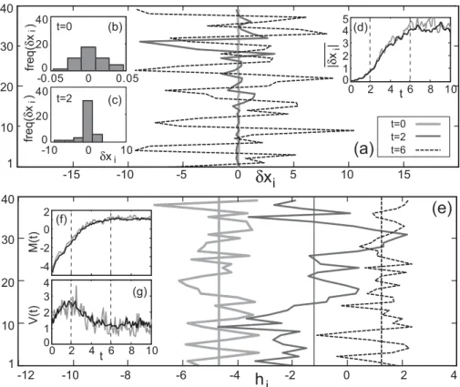
Figure 1a shows the evolution of the fluctuations δxi(t ) for three different time values t=0, 2 and 6, respectively. The perturbation was introduced at a random point of a Lorenz96 orbit, using normally distributed random values with zero mean and a 0.005 fraction of the variance of the system. Although the fluctuations are initially normally distributed, they quickly become peaked due to the multiplicative growth of perturbations resulting in a lognormal character. For in-stance, the insets (b)–(c) on the left show the frequency his-tograms of the fluctuations for t=0 and t=2, respectively; a Kolmogorov-Smirnov test applied to δxi(3) rejects the hy-pothesis of normality with a 95% confidence whereas it ac-cepts the hypothesis of log-normality with the same confi-dence. This major change of the spatial distribution is obvi-ated when considering the spatially averaged growth in time, which exhibits the typical exponential growth of chaotic tems until the fluctuations reach the amplitude of the sys-tem and saturate. Figure 1d shows the mean absolute growth (averaged spatially over i) showing this characteristic behav-ior; the gray line corresponds to a single fluctuation (a single member), whereas the dark line shows an ensemble average over 10 members, with a smooth behavior.

Motivated by the above lognormal behavior and with the aim to characterize both the temporal and spatial components of the spatiotemporal dynamics, L´opez et al. (2004) analyzed the logarithm of absolute values of perturbations

hi(t ) = ln(|δxi(t )|) (2)

and found that they evolve as kinetic roughening interfaces defined in space i and time t (for instance, Fig. 1e shows the logarithmic fluctuations for three values of time, t=0, 2 and 6). This type of processes can be characterized using the first two moments (mean and variance) which evolve according to precise fractal power laws related to characteristic mag-nitudes responsible of the spatiotemporal dynamics (spatial correlation, etc.):

– The spatial mean of the interface, given by

M(t ) = * 1 L L X i=1 hi(t ) + = * ln L Y i=1 |δxi(t )| !_L1+ , (3)

where the angle brackets mean ensemble aver-age, evolves in a characteristic linear regime as M(t )∼M(0)+λ t (where λ is the leading Lyapunov ex-ponent). Saturation is produced by the finite amplitude of the system, which becomes relevant in the nonlinear regime. The upper inset on Fig. 1e (panel f) shows these two characteristic regimes for a single member (gray line) and a 10-members ensemble (dark) (see L´opez et al. (2004) for more details).

0 2 4 6 8 10 0 1 2 3 4 -4 -2 0 2 -0.05 0 0.05 0 20 40 -10 0 10 0 20 40 2 4 0 -2 -4 -6 -8 -10 -12 10 5 0 -5 -10 15 -15

h

δx

i

i

(e)

(a)

Fig. 1. (a) Spatiotemporal growth of perturbations for three different values of time for a single member; the insets show the histograms for

two values of time (b, c) and the averaged spatial growth in time ((d), gray line). (e) Interface corresponding to the logarithmic fluctuations; the inset shows the spatial mean and variance of this single member (gray lines). The dark lines in insets (d), (f) and (g) correspond to ensemble averages over 10 members. Insets (b) and (c) are relative to the same single ensemble member as the main panels (a) and (e).

– The width (or roughness) of the interface, defined as the

variance of fluctuations around the spatial mean

V (t ) = hV ar(hi(t ))i = * 1 L L X i=1 (hi(t ) − h(t ))2 + . (4)

The overbar represents the spatial mean (i.e. average over i). This magnitude grows as a power-law of the form V (t )∼t2β in the linear regime. However, since the space is finite, the width saturates attaining a value depending on L, Vs(t )∼L2α. Moreover, in the nonlin-ear regime the variance decays due to nonlinnonlin-ear effects. The lower inset in Fig. 1e (panel g) shows this behav-ior, where nonlinear effects start acting at t=2 (for this particular initial amplitude). The above exponents are characteristic for certain families of processes sharing similar spatiotemporal behavior. In this case, fluctua-tions correspond to the so-called KPZ universality class and satisfy the additional constraint α=1/2, β=1/3 (see Barab´asi and Stanley (1995), for more details).

In the growth process a rough interface becomes a frac-tal curve. This fracfrac-tal structure, that is dynamically gener-ated, exhibits a strong spatial correlation over a characteristic length ℓc(t ).

The length ℓc informs about the extent on which the struc-ture behaves as fractal and can be easily measured by means of the correlation function (Primo et al., 2006) or the spa-tial power spectrum (Primo et al., 2007). This length and the roughness exponent α characterize the spatial structure of the rough interface. Note that in a mathematical context the roughness exponent is better known as the Holder expo-nent. Finally the dynamic process is characterized by an-other exponent that appears in the evolution of the structure as ℓc(t )∼t1/z. The z exponent is called the dynamic expo-nent. With this intuitive picture in mind we can understand the meaning of the variance. V (t ) is directly measuring the vertical growth of the rough curve but, since a fractal is a self-affine structure that relates both the vertical and horizontal scales as ℓvert=ℓαhor, it also measures the correlation length.

So, in the present case, the vertical scale can be measured by the standard deviation of the interface V1/2and, therefore: V1/2∼ℓα_c (i.e. V ∼ℓ2α_c ). In the KPZ universality class α=1/2 and V ∼ℓc. In any case, even for other roughness exponents both quantities are not independent and, therefore, the width of the interface characterizes both the spatial growth and the spatial correlation length of the perturbations.

Note that in spatiotemporal systems each spatial point evolves in connection with its neighbors creating correlated

112 J. M. Guti´errez: The MVL Spatiotemporal diagram

(b)

(a)

Non linear b arrier -6 -5 -4 -3 -2 -1 0 1 2 1.5 2 2.5 3 linearized system nonlinear system Random Bred vector

Fig. 2. (a) MVL diagram (see text) for the nonlinear Lorenz96

(solid) and the linearized system (dashed). (b) MVL diagram for two different initial perturbations: random (solid) and bred vectors (dashed).

structures which characteristic spatial scales. As shown by L´opez et al. (2004) the characteristic spatial scales of per-turbations evolve in time according to the laws of rough inter-faces and, moreover, can be analyzed considering the width of the interface, V (t ). Thus, whereas the mean M(t ) is only related to the temporal growth of perturbations (neglecting the spatial component), the width V (t ) is related to their changing spatial structure which is also responsible of the global growth, interplaying with the temporal component.

As a conclusion, both components have to be taken into account for a proper characterization of the growth or pertur-bations. In the next section we use these two components to define a diagram characterizing the spatiotemporal growth.

3 The MVL representation of ensembles

Motivated by the previous results, we consider a two-dimensional spatiotemporal growth diagram for the log-perturbations as follows. Along the horizontal axis we rep-resent M(t), which characterizes the temporal mean growth (leading Lyapunov exponent). Along the vertical axis, V (t ) characterizes the spatial growth and the correlation length (i.e. the degree of localization). We refer to this represen-tation as the Mean-Variance Logarithmic (MVL) diagram. In this diagram, the points evolve in time from left to right, since the mean of the perturbations always increases in time. However, the vertical dynamics is richer. The points move

upward as perturbations gain structure, and downward, when they lose structure (e.g., nonlinear effects due to finite ampli-tude appear).

To illustrate the MVL diagram we consider the Lorenz96 model (1) with a spatially uncorrelated random perturbation normally distributed with zero mean and a 0.5% of the vari-ance of a saturated perturbation. We generated an ensemble with N =10 members (as in Sect. 2). The perturbed initial condition xi(0)+δxi(0) is not projected into the attractor of the system (no real trajectory of the system passes through this point). Figure 2a shows the evolution, in the MVL dia-gram, of the log-perturbations in both the original nonlinear Lorenz96 system and the tangent linear version. Since the initial condition is uncorrelated, V is initially small. For a normal spatially uncorrelated initial perturbation, it can be shown that V is around 1.23 (namely, π2/8) regardless of the spatial size of the system or the amplitude of the initial perturbation. V starts growing as the system dynamically adapts the spatial structure of the perturbation (drives the or-bit towards the attractor of the system). In the linearized sys-tem, after some time the perturbation reaches the saturation regime, due to the space finiteness (L=40), and stays there forever. However, in the nonlinear case, the amplitude of the perturbation is bounded by the amplitude of the system and, thus, a “nonlinear barrier” appears and the system tends to an stationary point or zone (if the system is stationary). The diagram clearly shows the linear and nonlinear regimes and gives useful information regarding how the spatial structure is dynamically changed by the nonlinear system. This is the characteristic regime transition of initially random perturba-tions in nonlinear spatiotemporal systems.

In order to study the spatiotemporal evolution for different choices of the initial perturbations, we have also considered “bred vectors” (BV) as initial perturbations. BVs possess the typical spatial structure proper of the system and are pro-jected into the attractor. They are obtained as finite perturba-tions dynamically evolved in the nonlinear system (Toth and Kalnay, 1993).

Figure 2b shows the evolution of both the uncorrelated and breeding perturbations. They start from the same ver-tical line on the diagram since they were selected to share the same initial geometric amplitude, ρ(0)=Q |δxi(0)|

1

L_{. Their}

evolution is very different, though. BVs have a large ini-tial V value which indicates their appropriate spaini-tial struc-ture. Since they cannot increase their structure (they start saturated), they evolve keeping the space finiteness satura-tion value until they reach the non-linear saturasatura-tion. Both MVL trajectories meet at the non-linear barrier and end up at the same uncorrelated point of the diagram.

The space finiteness and non-linear barriers cannot be computed analytically and the only way to find them is by linearizing the system and let it reach a saturated state (space finiteness barrier) and by letting the non-linear system evolve until the non-linear effects appear, as plotted in Fig. 2.

4 Operational ECMWF ensembles

In this section we analyze two operative EPS generated at the ECMWF by means of fully featured coupled atmosphere-ocean global circulation models. On one hand, the seasonal EPS, based on simulations integrated for 120 days. The ini-tial perturbations are introduced in the SST and wind stress by using analog historical patterns. On the other hand, the monthly EPS (Vitart, 2004) fills the gap between the medium-range and the seasonal forecasting systems: it shares char-acteristics of both of them. Medium-range weather fore-casting is essentially an atmospheric initial value problem. It is based on atmospheric-only integrations and perturba-tions are introduced in the atmosphere using Singular Vec-tors (Molteni et al., 1996). Seasonal forecasting is also an initial value problem, but with much of the information con-tained in the initial state of the ocean. It is based on coupled ocean-atmosphere integrations and the perturbations are in-troduced in the SST and the wind stress. The monthly fore-casting system is also based on coupled ocean-atmosphere integrations, but produces forecasts for 30 days. This time range is probably still short enough that the atmosphere re-tains some memory of its initial state and it may be long enough that the ocean variability has an impact on the atmo-spheric circulation. Therefore, the perturbations are included in both the atmospheric and oceanic components using the above procedures.

Figure 3 shows the MVL diagram for the above ensembles corresponding to the same analysis day and using the daily geopotential at the 500 mb level. The values corresponding to different members are averaged in the diagram. Namely, the seasonal ensemble is composed of 40 members and the monthly ensemble of 50 perturbed members plus a control simulation. Additionally, there is a time average over a 3-month period including three seasonal initializations (they are initialized once per month) and 12 monthly simulations (one per week). The signature of the models in the MVL diagram is mostly insensitive to the initial conditions of the control simulation (not shown) since we are considering dif-ferences between model simulations and only the perturba-tions and the way they are grown into the model are relevant. There is a clearly apparent similarity with the diagram shown in Fig. 2. The initial degree of localization depends on the EPS considered. The monthly EPS shows a saturated spatial pattern which agrees with the initial perturbation in-troduced (an optimized singular vector consistent with the dynamics of the system). The seasonal EPS is only perturbed at the surface (SST and wind) so the perturbation at 500 mb is initially much smaller than for the monthly EPS (starts more to the left). Moreover, the surface perturbation appears as near-random from the 500 mb level and the small structure it possesses (localization slightly over the random, 1.23, value) is not projected into the attractor (corresponds to an analog from a different time) and is destroyed (localization starts going downward) before gaining the correct structure for the

Monthly Seasonal M(t) V(t) 3 4 5 6 7 8 1.1 1.2 1.3 1.4 1.5 1.6

Fig. 3. MVL diagram of the ensemble evolution for two different

operative models: monthly (black) and seasonal (gray). The dots on the lines show the time evolution; each dot represents a forecast day

system at that time.

The information given by the diagram can be used to test initialization procedures and assess the degree of localiza-tion reached by each one. For short range weather forecasts, it is important that the initial conditions lay on the attractor, thus avoiding the transient states where the model is trying to damp the solution to a dynamical state of the system. Each model has a different signature on the MVL diagram, so the comparison of initialization techniques should be carried out on the same model. Therefore, the diagrams for the bred vec-tors on the Lorenz96 model and the singular vecvec-tors on the ECMWF monthly EPS, shown in the present study, cannot be used to compare these techniques. That particular study is left for a forthcoming paper focused on the comparison of these initialization procedures.

It is important to remark that, in this diagram, when the ensemble saturates and decays to the stationary area, it loses all the information about the initial condition. At this point the saturated perturbations behave as random climatologi-cal values. In this particular example, this occurs after two weeks for the seasonal EPS and after 10 days in the monthly EPS. Unlike the Lorenz96 model, in this case the saturation point becomes an area, since the coupled atmosphere-ocean system includes driving phenomena with long time scales. Therefore, the fluctuations around this area can be consid-ered climatological fluctuations.

5 Conclusions

This paper shows that very useful information of the spa-tiotemporal evolution of perturbations is obtained using an analogy with kinetic rough interfaces introduced by L´opez et al. (2004). We show that, in addition to the temporal growth, the spatial correlation, which grows and decays in time, plays a central role in the dynamics of perturbations. The main contribution of the paper is the MVL diagram which represents the spatio-temporal evolution of ensembles

114 J. M. Guti´errez: The MVL Spatiotemporal diagram of perturbations and allows a simple view of important

as-pects of the dynamics: growth, spatial correlation and pre-dictability.

The initial location in the horizontal axis only depends on the initial amplitude of the perturbations and, thus, it is an arbitrary value (in practice this value is chosen in con-nection with the error-of-the-day). The novel and most rel-evant part of the diagram is the vertical axis, represent-ing the spatial structure of the system. Note that the posi-tion of the initial condiposi-tion in the vertical axis can also be changed; for instance, we can move it upwards by introduc-ing spatially-correlated perturbations, instead of uncorrelated random ones. However, the perturbations will only preserve (or even increase) the vertical value as time goes by if the initial structure was coherent with the background flow (i.e., if the perturbed initial condition is on the attractor of the sys-tem); otherwise, the system will assimilate it progressively destroying the correlation to create a new assimilated one. Therefore, the diagram helps to assess whether the perturbed initial conditions are already assimilated into the dynamics.

The lorenz96 system allowed us to easily generate large ensembles with different kinds of initial perturbations (ran-dom and breeding vectors) which show different evolutions on the MVL diagram. The operational EPS products from ECMWF showed the expected MVL trajectories in terms of the underlying theory of the spatiotemporal evolution of per-turbations. There are clear similarities between the MVL trajectories of the simple Lorenz96 system and the complex global climate models.

Three different characteristic regimes in the MVL diagram characterize different features of the model dynamics and ini-tialization procedure. The initial stages characterize the per-turbation procedure. Spatially random, structured and struc-tured and dynamically assimilated initial perturbations are easily identifiable. The middle stages characterize how the linearized system amplifies the initial fluctuations in space and time. The longest the model stays at this stage, the slow-est the perturbations grow in time. Finally, the last stage pro-vides information on the climatological features of the satu-rated fluctuations as evolved by the non-linear system. The MVL diagram provides a signature of the model dynamics subject to an initial perturbation. As such, it could be used for model comparison.

The MVL diagram provides useful information about the type of perturbations used in numerical weather predictions, and characterizes the spatiotemporal dynamics from the ini-tial condition to the stationary zone where the information about the initial conditions is lost. It could be of great use for optimizing the generation of initial perturbations for EPS and also to compare the models from a dynamical point of view. Although further research is necessary in order to fully validate the usefulness of this representation, the examples provided in this paper are promising.

Acknowledgements. The authors are grateful to the Comisi´on Interministerial de Ciencia y Tecnolog´ıa (CICYT, CGL2005-06966-C07-02/CLI and CGL2007-64387/CLI grants) for partial support of this work. C. Primo and J. Fern´andez are supported by the Spanish Ministry of Education and Science through the Postdoctoral and Juan de la Cierva programs, respectively. Edited by: O. Talagrand

Reviewed by: Two anonymous referees

References

Barab´asi, A. L. and Stanley, H. E.: Fractal Concepts in Surface Growth, Cambridge University Press, 1995.

Gneiting, T. and Raftery, A.: Weather Forecasting with Ensemble Methods, Science, 310, 248–249, 2005.

Hagedorn, R., Doblas-Reyes, F. J., and Palmer, T.: The rationale behind the success of multi–model ensembles in seasonal fore-casting – I. Basic concept, Tellus, 57A, 219–233, 2005. L´opez, J. M., Primo, C., Rodr´ıguez, M. A., and Szendro, I.: Scaling

Properties of Growing Noninfinitesimal Perturbations in Space-Time Chaos, Phys. Rev. E., 70, 056224, 2004.

Lorenz, E. N.: Predictability-a problem partly solved. in Proceed-ings of ECMWF seminar Predictability., ECMWF Seminar Pro-ceedings, ECMWF, Reading, UK., Seminar on Predictability, 1, 1–19, 1996.

Lorenz, E. N. and Emanuel, K.: Optimal sites for supplementary weather observations: Simulation with a small model., J. Atmos. Sci., 55, 399–414, 1998.

Molteni, F., Buizza, R., Palmer, T., and Petroliagis, T.: The ECMWF Ensemble Prediction System: Methodology and vali-dation, Q. J. Roy. Meteorol. Soc., 122, 73–119, 1996.

Palmer, T. N.: The economic value of ensemble forecasts as a tool for risk assessment: From days to decades, Q. J. Roy. Meteorol. Soc., 128, 747–774, 2002.

Palmer, T. N., Alessandri, A., Andersen, U., Cantelaube, P., Dav-eyand, M., D´el´ecluse, P., D´equ´e, M., D´ıez, E., Doblas-Reyes, F. J., Feddersen, H., Graham, R., Gualdi, S., Gu´er´emy, J. F., Hagedorn, R., Hoshen, M., Keenlyside, N., Latif, M., Lazar, A., Maisonnave, E., Marletto, V., Orfila, A. P. M. B., Rofel, P., Ter-res, J. M., and Thomson, M. C.: Development of a European multimodel ensemble system for seasonal–to–interannual pre-diction DEMETER, B. Am. Meteorol. Soc., 85, 853–872, 2004. Primo, C., Szendro, I. G., Rodriguez, M. A., and L´opez, J. M.: Dynamic scaling of bred vectors in spatially extended chaotic systems, Europhys. Lett., 76, 767–773, 2006.

Primo, C., Szendro, I., Rodr´ıguez, M. A., and Guti´errez, J. M.: Er-ror growth analysis in systems with spatial chaos: Coupled map lattices and global weather models, Phys. Rev. Lett., 98, 108501, 2007.

Smith, L.: Disentangling uncertainty and error: On the predictabil-ity of nonlinear systems, Birkhauser, Boston, 2000.

Toth, Z. and Kalnay, E.: Ensemble Forecasting at NMC: The Gen-eration of Perturbations, B. Am. Meteorol. Soc., 74, 2317–2330, 1993.

Vitart, F.: Monthly forecasting at ECMWF, Mon. Weather Rev., 132, 2761–2779, 2004.

Wilks, D. S.: Effects of stochastic parameterization in the Lorenz 96 system, Q. J. Roy. Meteorol. Soc., 131, 389–407, 2005.