From accelerometric records to the dynamic behavior of existing buildings

HAL Id: tel-01627564

https://tel.archives-ouvertes.fr/tel-01627564v2

HAL is a multi-disciplinary open access archive for the deposit and dissemination of sci-entific research documents, whether they are pub-lished or not. The documents may come from teaching and research institutions in France or abroad, or from public or private research centers.

L’archive ouverte pluridisciplinaire HAL, est destinée au dépôt et à la diffusion de documents scientifiques de niveau recherche, publiés ou non, émanant des établissements d’enseignement et de recherche français ou étrangers, des laboratoires publics ou privés.

existing buildings

Guillermo Wenceslao Fernandez Lorenzo

To cite this version:

Guillermo Wenceslao Fernandez Lorenzo. From accelerometric records to the dynamic behavior of existing buildings. Other. Université Côte d’Azur, 2016. English. �NNT : 2016AZUR4071�. �tel-01627564v2�

École Doctorale de Sciences Fondamentales et Appliquées Unité de recherche : Géoazur / LJAD

Thèse de doctorat

de

l’UNIVERSITE COTE D’AZUR

par

Guillermo Wenceslao FERNÁNDEZ LORENZO

From accelerometric records

to the dynamic behavior

of existing buildings

Des données accélérométriques

au comportement dynamique

des bâtiments existants

Dirigée par Anne DESCHAMPS et Maria Paola SANTISI D’AVILA

Soutenue le 17 Octobre 2016 Devant le jury composé de :

Etienne BERTRAND Chargé de recherche, CEREMA Conseiller d’étude Françoise COURBOULEX Directeur de recherche, CNRS Président du jury Anne DESCHAMPS Directeur de recherche, CNRS Directeur de thèse Philippe GUÉGUEN Directeur de recherche, IFSTTAR Rapporteur

Luca LENTI Chargé de recherche, IFSTTAR Examinateur

E. Diego MERCERAT Chargé de recherche, CEREMA Examinateur Maria Paola SANTISI D’AVILA Maître de conférence, UNS Directeur de thèse Jean-François SEMBLAT Directeur de recherche, IFSTTAR Rapporteur

Earthquakes don’t kill people, collapsed buildings do. . .

— UNOPS

To my parents

Acknowledgements

I start by saying merci to Fred. You supported me during all this time and without you I would probably not be here. Je t’aime.

Thanks to Paola, Anne, my supervisors, for your patience, encouragement and guidance throughout these years.

Thanks to the members of my doctoral committee, to my rapporteurs Jean Francois and Philippe and examinateurs Luca and Francoise for having accepted to take the time to read and comment my thesis work. Specially to Philippe for having received me at Grenoble. A special thank to Diego and Etienne for your unofficial guidance, advice, and for keeping me motivated when the work became harder. Thank to Julie and the rest of the CEREMA team (Nathalie, Simon, David, etc.) for all the coffee discussions we shared.

Thanks to everyone at Geoazur, researchers, students and technical staff. A special mention to Maelle, Edouard, companions of adventures and parties, respectively, and the rest of the doctorants team (Mathilde, Stephen, Sadrac, Alex, Sargis, Chloé, etc.) for making the lab a great place to pass by.

Thanks to the participants of the JDPN and their organizers. The seminar ’from doctorants to doctorants’ where scientific research, fun and friendship can always be found. Thanks to the members of the group jeunes de l’AFPS (Cedric, Celine, etc.), a great starting point to get into the para-seismic community.

Thanks to Piero, who initiated me to earthquake engineering and who encouraged me to pursue this thesis in Nice.

I wish to express my deep gratitude to the Provence Alpes Côte d’Azur region, that has founded this thesis trough a 3-year doctoral contract as a result of a strong interaction with the CEREMA partner.

Finally, thanks to my mother Margarita, and my brothers, Alfonso and Santiago, my closer family, who always supported me, in as many ways as possible.

Abstract

The aim of this thesis is to simulate the time history response of a high rise building under seismic excitation and provide simplified methodologies that properly reproduce such re-sponse. Firstly, a detailed three-dimensional finite element model is produced to validate its reliability to simulate the real behavior of the building during ground motions, recorded using accelerometers. It is proposed to improve the accuracy of the numerical model by imposing multiple excitations, considering rocking effect and spatial variability on the input motion. The finite element model provides excellent results when dynamic parameters are calibrated to match the service condition of the structure.

The use of empirical Green’s functions is proposed to simulate the seismic response directly from past event records, without the need of construction drawings and mechanical parame-ters calibration. A stochastic summation scheme, already used to predict ground motions, is adopted to generate synthetic signals at different heights of the building, extending the wave propagation path from the ground to the structure. The procedure shows good agreement with numerical signals provided by the finite element model.

A simplified representation of the building as a homogeneous Timoshenko beam is proposed to simulate the seismic response directly from ambient vibration records. Equivalent mechan-ical parameters are identified using deconvolution interferometry in terms of wave dispersion, natural frequencies, and shear to compressional wave velocities in the medium. Response simulation of lower modes, up to the fifth natural frequency, is properly reproduced by the equivalent model.

Both proposed techniques provide alternatives to finite element modeling, when in-situ records (either seismic or ambient noise) are available, to avoid difficulties related with the lack of data about structure and materials and computing time.

Keywords: seismic response simulation, high rise building, operational modal analysis, finite

Contents

Acknowledgements i

Abstract iii

List of figures ix

List of tables xvii

1 General introduction 1

2 Basis concepts of structural dynamics and background of building instrumentation 7

2.1 Structural dynamics . . . 8

2.1.1 Equation of motion . . . 8

2.1.2 Free vibration . . . 9

2.1.3 Harmonic excitation . . . 12

2.1.4 Seismic response . . . 15

2.1.5 Effects of SSI on natural frequencies . . . 18

2.1.6 MDOF systems . . . 19

2.1.7 Euler–Bernoulli beam . . . 22

2.1.8 Timoshenko beam . . . 24

2.2 Instrumentation of buildings . . . 26

2.2.1 Vibrational analysis of buildings . . . 26

2.2.2 Seismic ambient noise . . . 29

2.2.3 Ambient vibrations in buildings . . . 30

3 Structural identification: the Nice prefecture building 33 3.1 Introduction . . . 34

3.2 Case study of the Nice prefecture . . . 35

3.2.1 Description of the structure . . . 35

3.2.3 Geotechnical context . . . 37

3.2.4 Regional and national seismicity . . . 38

3.3 Identification of dynamic properties from records . . . 40

3.3.1 Comparison of accelerometric and velocimetric data . . . 40

3.3.2 Basic frequency domain . . . 42

3.3.3 Frequency domain decomposition . . . 43

3.3.4 Random decrement . . . 47

3.3.5 Natural frequencies and mode shapes of the building . . . 47

3.4 Finite element model of the building . . . 49

3.4.1 Creation of a model of an existing structure . . . 50

3.4.2 Structural modeling from construction plans . . . 51

3.4.3 Model optimization using operational modal analysis . . . 51

3.4.4 Effects of seismic joint on dynamic properties . . . 52

3.5 Variation of dynamic parameters with environmental conditions . . . 53

3.6 Conclusions . . . 57

4 Response simulation using finite elements: relevance of the spatial variability of the input motion 61 4.1 Introduction . . . 62

4.2 Recorded earthquakes . . . 62

4.2.1 2012 and 2014 Barcelonnette earthquakes . . . 62

4.2.2 Variation of building frequencies during ground motion . . . 63

4.3 Imposition of a single tri-axial input load (SI) . . . 67

4.4 Imposition of multiple input loads (MI) . . . 70

4.5 Quantitative comparison of goodness of fit: SI vs MI . . . 73

4.6 Conclusions . . . 78

5 Response prediction from records: application of empirical Green’s function approach to buildings 81 5.1 Introduction . . . 82

5.2 Seismic response at any story from records at the roof: KY formulation . . . 84

5.3 Principles of the EGF method . . . 86

5.3.1 Selection criteria for a small event . . . 86

5.3.2 Applicability conditions . . . 88

5.3.3 Stochastic summation scheme . . . 89

5.4 Generation of reference ground motion . . . 90 vi

Contents

5.5 Generation of building deformation time histories . . . 92

5.5.1 Qualitative comparison . . . 92

5.5.2 Quantitative comparison . . . 94

5.5.3 Prediction at any story from records at the top of the building . . . 95

5.6 Actual limitations of the semi-empirical approach . . . 95

5.7 Conclusions . . . 99

6 Identification of mechanical parameters from ambient vibration interferometry: mod-eling buildings as fixed-base Timoshenko beams 101 6.1 Introduction . . . 102

6.2 Application of interferometry to buildings . . . 105

6.3 Equivalent beam model of a building . . . 105

6.3.1 Case study . . . 107

6.3.2 Timoshenko beam model . . . 108

6.3.3 Fundamental frequencies of a 3D Timoshenko beam . . . 112

6.4 Information obtained from records . . . 115

6.4.1 Transfer function and deconvolution procedure . . . 115

6.4.2 IRFs for building identification . . . 118

6.4.3 Estimation of compression to shear wave velocity ratio . . . 122

6.4.4 Dispersion images of recorded IRFs . . . 122

6.5 Identification of mechanical parameters for the equivalent model . . . 127

6.6 Response simulation using a Timoshenko beam . . . 129

6.6.1 Qualitative comparison . . . 130

6.6.2 Quantitative comparison . . . 130

6.7 Conclusions . . . 133

7 Global conclusions and perspectives 137

Bibliography 157

Résumé étendu de la thèse 159

List of Figures

2.1 Representation of a single degree of freedom oscillator (from Gavin, 2014). . . . 8 2.2 Representation of a single degree of freedom oscillator subjected to ground

motion (from Gavin, 2014). . . 9 2.3 Free vibration of underdamped (ξ < 1), critically damped (ξ = 1) and

over-damped (ξ > 1) systems (from Chopra, 2012). . . 12 2.4 Response of undamped (a) and damped (ξ = 0.05) (b) systems to harmonic force

ω/ωn= 0.2, with u(0) = 0 and ˙u(0) = ωnp0/k (from Chopra, 2012). . . . 13

2.5 Response of undamped (a) and damped (ξ = 0.05) (b) systems to sinusoidal force of frequencyω = ωn, with u(0) = 0 and ˙u(0) = 0 (from Chopra, 2012). . . . 14

2.6 Deformation response factor and phase angle for a damped system excited by harmonic force (from Chopra, 2012). . . 15 2.7 Ground motions recorded during several earthquakes (from Chopra, 2012). . . 16 2.8 One degree of freedom base model for: (a) system on a elastic soil, (b) discrete

system where base compliance is represented by springs and dashpots, (c) com-ponents of motion of base and mass (from Kramer, 1996). . . 18 2.9 Variation of frequency ratios fn/ f1for modes above the fundamental frequency

with the dimensionless parameter C , for a continuous Timoshenko beam. Grey areas represent the limit for bending and shear beam behavior (Michel, 2007). . 26 3.1 (a) Front view of the Nice prefecture building (CETE, 2010). (b) Horizontal

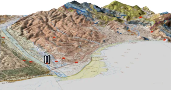
section of the RC tower to which RC shells are connected at each floor and of vertical columns (from structural plans). (c) Distribution of sensors along the instrumented tower. Red and green arrows represent monoaxial and triaxial accelerometers, respectively (CETE, 2010). . . 36 3.2 Location of the building in the Var valley. Building is not to scale (adapted from

Bertrand et al. 2014). . . 38 3.3 2010 French seismic zonation map (modified from LEGIFRANCE, 2010). . . 39

3.4 Europe earthquakes in the SHARE European Earthquake Catalog (SHEEC) be-tween years 1000 - 2007 with moment magnitudes MW≤ 3.5 (from Cameelbeeck

et al., 2013). . . 39 3.5 Episensor FBA EST tri-axial accelerometer (a) and CGM40 tri-axial velocimeter

(b) used for the comparison. . . 41 3.6 Contour plots of cross correlation coefficient between accelerometer and

ve-locimeter recordings for different passband cutting frequencies. Red and green crosses highlight values for 0.4-25 Hz and 1-10 Hz passband filters respectively 42 3.7 Amplitude of the frequency spectrum for the HN2 (blue) and HN3 (red)

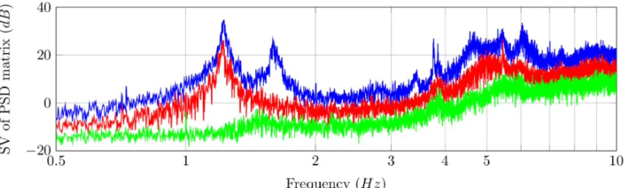
compo-nents of acceleration recorded at the top of the building (V0) . . . 43 3.8 1st (blue), 2nd (red) and 3r d (green) Singular Values of the of the PSD matrix

from FDD technique . . . 46 3.9 Mode shapes of the instrumented tower, for the first five natural modes, using

FDD. . . 46 3.10 Records of the Nice prefecture (filtered around the fundamental mode) that

satisfy the null displacement and positive velocity initial conditions (black) are averaged to obtain the random decrement signature (red). Damping is obtained by fitting a logarithmic function to the envelop of the signature (blue). . . 48 3.11 1st and 2nd Singular Values (SV) of the Power Spectral Density (PSD) matrix

using FDD. Proposed frequency bands (B2, B3, B4, B5) to individually study isolated natural frequencies. . . 49 3.12 First three mode shapes obtained by the finite element model considering

in-dependent dynamic behavior of the two towers (FEM1). Colormap show the normalized displacement of nodes. . . 52 3.13 First three mode shapes obtained by the finite element model considering a

rigid connection between towers (FEM2). Colormap shows the normalized displacement of nodes. . . 54 3.14 Variation of fundamental frequency (f0HN3 RD) and temperature during one

week at the outside (UKO V0) and the inside (UKI A0) of the building. Tem-perature axis is inverted to highlight the negative correlation of fundamental frequency and outer temperature. Days of the week are specified and the week-end is highlighted with a light red. . . 55 3.15 Variation of fundamental frequency (f0HN3 RD) and temperature during one

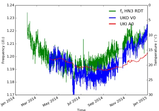
year at the outside (UKO V0) and the inside (UKI A0) of the building. Temperature axis is inverted to highlight the negative correlation of fundamental frequency and outer temperature. . . 56 x

List of Figures

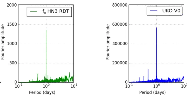
3.16 Fourier transform of one year of measures of the fundamental frequency, f0,

us-ing RD (left) and ambient temperature at the top of the buildus-ing (right). Remark that the abscissa axis is shown in terms of period (inverse of frequency). . . 57 3.17 Smoothed variation of fundamental frequency (f0HN3 RD) and temperature

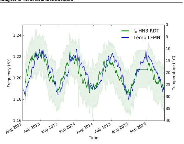
at the LFMN meteorological station (less than 1km to the building) since 2012. One standard deviation of measures is represented with a lighter color. . . 58 3.18 Fourier transform of four years of measures of the fundamental frequency, f0,

using RD. Remark that the abscissa axis is shown in terms of period (inverse of frequency). . . 58

4.1 Catalog of events properly recorded at the Prefecture building since it was in-strumented (according to the RENASS catalog). Evaluation of recorded signal quality is carried out using a STA/LTA trigger. . . 63 4.2 Recorded accelerograms at different locations (A0, A1, A2) at the base of the

building, for the two horizontal (HN2, HN3) and vertical (HNZ) components, during the 2012 Mw4.2 (left) and 2014 Mw4.9 (right) Barcelonnette earthquakes. 64

4.3 Macrosismic intensity (EMS98) of the 26 February 2012 (left) and 7 April 2014 (right) Barcelonnette earthquakes. Modified from BCSF Sira et al. (2012, 2014). 64 4.4 Variation of fundamental modes in the Millikan library. Dashed lines represent

the natural frequencies associated to the traslational shape mode in E-W direc-tion and the dashed-dotted lines represent the natural frequencies associated to the translational shape mode in N-S direction. Shaded area is the likely range of natural frequencies taking into consideration errors in measurement due to various factors - weight configuration in the shaker, weather conditions at the time of the test, and experimental error. Crosses indicate actual time forced test was made. Circles indicate natural frequency estimates from the strong motion record during earthquake events, and numbers in italics are peak acceleration recorded for the event (cm/s2). [Earthquake Abbreviations: LC: Lytle Creek, SF: San Fernando, WN: Whittier Narrows, SM: Santa Monica, NR: Northridge, BH: Beverly Hills, BB: Big Bear] (adapted from Clinton 2004). . . 65 4.5 Fourier transform of the recorded acceleration at the top of the building under

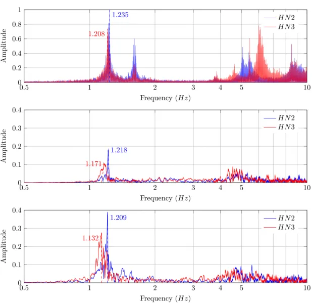
ambient vibrations (top), during the 2012 Barcelonnette earthquake (middle) and during the 2014 Barcelonnette earthquake (bottom). The value of the first bending mode on each direction (HN2, HN3) is highlighted. . . 66

4.6 Numerical simulation of the building by imposing a tri-axial signal recorded at A0 at the base of the model. Time-histories of horizontal acceleration (HN2, HN3) are obtained at the top of the building (V0). . . 67 4.7 Recorded (REC) and numerical (FEM) horizontal acceleration (HN3) at the top

of the building (V0) during the 2012 Barcelonnette earthquake for different frequency bands. One triaxial signal is used as input in the numerical model. . 68 4.8 Recorded (REC) and numerical (FEM) horizontal acceleration (HN3) at the top

of the building (V0) during the 2014 Barcelonnette earthquake for different frequency bands. One triaxial signal is used as input in the numerical model. . 69 4.9 Time window of the three components (HN2, HN3, HNZ) of 2014 Barcelonnette

earthquake, recorded at different points at the base of the building (A0, A1, A2). 70 4.10 Numerical simulation of the building by imposing multiple input (MI) signals at

different points of the base of the model (A0, A1, A2). Time-histories of horizontal acceleration (HN2, HN3) are obtained at the top of the building (V0). . . 71 4.11 Recorded (REC) and numerical (FEM) horizontal acceleration (HN3) at the top

of the building (V0) during the 2014 Barcelonnette earthquake for different fre-quency bands. Multiple recorded signals are simultaneously applied at different points of the base of the building in the numerical model. . . 72 4.12 Short time Fourier transform of the horizontal HN3 (left) and vertical HNZ (right)

acceleration at the base of the building (A0) during the 2014 Barcelonnette earthquake. . . 72 4.13 Short time Fourier transform of the horizontal HN3 acceleration at the top of the

building (V0) during the 2014 Barcelonnette earthquake for records (left) and FE simulation (right). . . 73 4.14 Values of Anderson parameters for comparison with records of a horizontal

component (HN3) at top of the building (V0), during the Barcelonnette 2014 earthquake, for the cases of modeling with an imposed mono-axial signal (SI) and multiple signals (MI). . . 75 4.15 Comparison of the Fourier spectrum (FS) and Arias intensity (AI) for a horizontal

component (HN3) at top of the building (V0), during the Barcelonnette 2014 earthquake, for the cases of modeling with an imposed mono-axial signal (SI) and multiple signals (MI). . . 75 xii

List of Figures

4.16 Anderson’s GoF scores for numerical horizontal component (HN3) at the top of the building (V0) during the 2012 (top) and 2014 (bottom) Barcelonnette earthquakes compared with records, in different frequency bands, in both cases of a single three-component signal applied as input to the whole base (SI) and multiple signal input (MI). Evaluated parameters include Arias duration (AD), energy duration (ED), Arias intensity (AI), energy integral (EI), peak acceleration (PA), peak velocity (PV), peak displacement (PD), pseudo-acceleration floor response spectra (Sa) and Fourier spectra (FS) and cross correlation (C*). . . 76 4.17 Comparison of Arias integral, energy integral, elastic response spectrum in terms

of pseudo-acceleration and Fourier spectrum for the horizontal acceleration component HN3 at the top of the building (V0), during the 2014 Barcelonnette earthquake: records (REC), FE model with single-input (SI) and FE model with multi-input (MI). . . 77

5.1 HN3 horizontal component of structural deformation at different heights of the building, both recorded (REC) during the 2014 Barcelonnette earthquake and deduced using the record at the top of the building according to the revisited Kanai-Yoshizawa formulation (KY). . . 87 5.2 Principle of the strong motion generation trough empirical Green’s functions:

the records of a single small earthquake are combined several times to produce synthetic recordings for a larger event at a given station (from Courboulex (2010)). 88 5.3 HN3 acceleration component, recorded (REC) at the base of the building (A0)

during the 2012 Mw4.2 and 2014 Mw4.9 Barcelonnette earthquakes and

gener-ated for the two Mw6 earthquakes (EGF) using 2012 and 2014 events as EGF. . 91

5.4 Acceleration response spectra for HN3 component of motion, recorded (REC) at the base of the building (A0) during the 2012 Mw 4.2 and 2014 Mw4.9

Barcelon-nette earthquakes and generated for the two Mw6 earthquakes using 2012 and

2014 events as EGF. The fundamental period of the structure is highlighted by a dashed line. . . 91 5.5 HN3 horizontal acceleration component at the top of the building (V0), for

differ-ent frequency bands: synthetic signal provided by EGF for a Mw 6 earthquake in

Barcelonnette using 2014 event as small earthquake (EGF) and numerical signal obtained by the FE model with a synthetic ground motion as multiple input at the base (EGF+FEM) corresponding to a Mw 6 earthquake in Barcelonnette. . . 93

5.6 Short time Fourier transform of the horizontal acceleration component HN3 at the top of the building (V0) given by EGF+FEM (left) and EGF (left) for a Mw6

earthquake in Barcelonnette. . . 94 5.7 Anderson’s GoF scores for the comparison of the horizontal acceleration

com-ponent HN3 at the top of the building (V0), obtained by EGF and EGF+FEM in the case of a Mw 6 earthquake in Barcelonnette, for different frequency bands.

Evaluated parameters include Arias duration (AD), energy duration (ED), Arias intensity (AI), energy integral (EI), peak acceleration (PA), peak velocity (PV), peak displacement (PD), pseudo-acceleration response spectra (Sa) and Fourier spectra (FS) and cross correlation (C*). . . 94 5.8 Comparison of Arias integral, energy integral, elastic response spectrum in

terms of pseudo-acceleration and Fourier spectrum for the HN3 horizontal acceleration component in the cases of synthetic signals generated at the top (V0) of the building (EGF) and numerical signals obtaining usisng EGF as seismic loading (EGF+FEM), during the reference Mw6 earthquake in Barcelonnette. . 96

5.9 Comparison of HN3 horizontal component of structural deformation at different heights of the building generated applying EGF procedure to records at the floor level (EGF) and approximated using Kanai-Yoshizawa formulation to EGF simulation at the top of the building (EGF + KY) related to the reference Mw 6

earthquake in Barcelonnette. . . 97 6.1 Interferograms using records of the 2014 Barcelonnette earthquake deconvolved

with respect to the sensor at the bottom (a) and by the sensor at the top of the building (b). The identification of the propagation path from the acausal and causal waves to estimate the wave velocity is shown in blue and red, respectively.106 6.2 (a) Perspective view of the Nice prefecture building. (b) Horizontal section of

building structure. . . 107 6.3 Shear (a) and bending (b) type structural behavior of a building under seismic

loading. . . 108 6.4 (a) Cantilever Timoshenko beam equivalent to the analyzed building. (b) Free

body diagram of a beam segment. . . 109 6.5 Variation of the dispersion curve with the elasticity modulus to density ratio for

a beam of 66 m long, H , with rectangular cross-section of different width, b, and a constant depth, h, of 40m. . . 111 6.6 Two first singular values of power spectral density obtained using the frequency

domain decomposition analysis for the studied building. . . 116 xiv

List of Figures

6.7 Horizontal acceleration recordings (HN2 component) at different floors of the building during (a) the 2014 Mw 4.9 Barcelonnette earthquake and (b) 60s of ambient vibration. . . 117 6.8 Impulse response functions of the recorded HN2 component of motion,

ob-tained by deconvolution with respect to the signal at the base (a) and top (b) of the building during the 2014 Mw 4.9 Barcelonnette earthquake and at the base

(c) and top (d) of the building during 60 s of ambient vibration. High frequencies are removed for clarity purpose using a 10 Hz low pass filter. . . 118 6.9 Impulse response functions obtained by deconvolution with respect to the signal

at the top of the building, filtering the signal in two different frequency bands. Thick lines represent the trajectory of causal waves by picking the phase lag time arrival at the bottom. . . 120 6.10 Smoothed variation of wave velocity, fundamental frequency and temperature

during three days. One sample per minute is calculated. . . 121 6.11 Smoothed impulse response functions obtained using deconvolution with a

virtual source at the top of the building, for different propagation directions (HN2, HN3, HNZ). Data have been acquired during a temporary instrumentation campaign where velocimeters have been used. Wave propagation arrival times are picked and the propagation paths are indicated. . . 123 6.12 Normalized wave velocity image with a virtual source at the bottom of the

build-ing. Considered frequency-wavenumber resolution limits are shown with a dashed line. . . 125 6.13 Normalized wave velocity image with a virtual source at the top of the building.

Frequency-wavenumber resolution limits are shown with dashed lines. Wave velocities estimated using resonant frequencies are highlighted by points and those points using picked phase arrival times by thick lines. Fitted analytical solution of the Timoshenko beam dispersion curve is shown using a thin straight line. . . 126 6.14 Normalized transfer functions (left) and velocity spectrums (right), for the HN2

(up) and HN3 (down) horizontal components of the building motion. Natural frequencies (dash-point lines) of the building and analytical dispersion curve (straight line). Frequency-wavenumber resolution limits (dashed line). Picked shear wave velocities (dotted line). . . 129

6.15 Numerical response in terms of horizontal acceleration (HN3) at the top (V0) of the detailed 3D model of the building (FEM-SI) and the equivalent Timoshenko beam (TB) under the three components of the 2014 Barcelonnette earthquake for different frequency bands. . . 131 6.16 Anderson’s GoF scores for the comparison of the horizontal acceleration

compo-nent HN3 at the top of the building (V0), obtained by an equivalent Timoshenko beam (TB) and a detailed three-dimensional model (FEM-SI) during the 2014 Barcelonnette earthquake, for different frequency bands. Evaluated parameters include Arias duration (AD), energy duration (ED), Arias intensity (AI), energy integral (EI), peak acceleration (PA), peak velocity (PV), peak displacement (PD), pseudo-acceleration response spectra (Sa) and Fourier spectra (FS) and cross correlation (C*). . . 131 6.17 Comparison of Arias integral, energy integral, elastic response spectrum in terms

of pseudo-acceleration and Fourier spectrum for the horizontal acceleration component HN3 at the top of the building (V0), during the 2014 Barcelonnette earthquake: numerical simulations using an equivalent Timoshenko beam (TB) and a detailed three-dimensional model (FEM-SI). . . 132 6.18 6t hto 12t h obtained using the finite element model under the hypothesis of

independent dynamic behavior of the two towers (FEM1). Colormap shows the normalized displacement of nodes. . . 133 6.19 Numerical response in terms of horizontal displacement (HN3) at the top (V0) of

the detailed 3D model of the building (FEM-SI) and the equivalent Timoshenko beam (TB) under the three components of the 2014 Barcelonnette earthquake for different frequency bands. . . 134

List of Tables

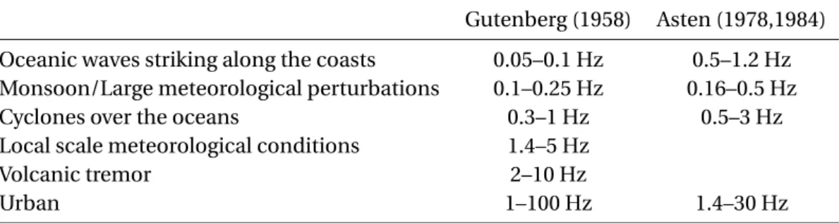
2.1 List of selected USGS extensively instrumented buildings (adapted from Dunand et al., 2004). . . 28 2.2 Summary of ambient noise sources according to frequency. Summary

estab-lished after studies by Gutenberg (1958), Asten (1978) and Asten and Henstridge (1984) (modified from Bonnefoy-Claudet et al. (2006)). . . 30

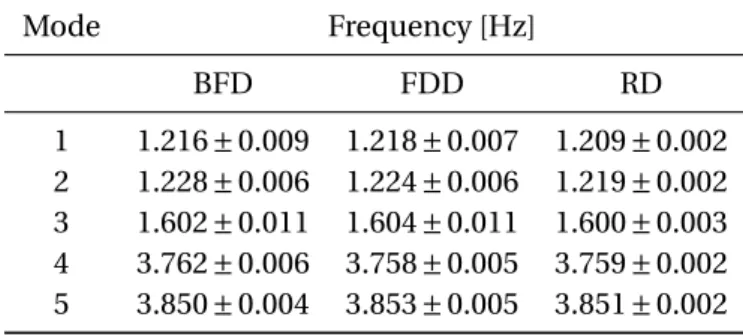
3.1 Natural frequencies of the building identified using BFD, FDD and RD. . . 48 3.2 Modal damping under noise excitation using RD. . . 49 3.3 Frequency bands that allows to individually observe the frequency content of

each mode in the case study. . . 49 3.4 Adopted values of density (ρ), Young modulus (E), Poisson’s ratio (ν) for the

reinforced concrete material. . . 51 3.5 First three natural frequencies f obtained by records (REC) and by the finite

element model for both independent behavior between towers (FEM1). Relative error² between FEM and REC. . . 52 3.6 First three natural frequencies f obtained by records (REC) and by the finite

element model considering a rigid connection between towers (FEM2). Relative error² between FEM2 and REC. . . 53

4.1 Natural frequencies variation with nature of input motion, measured as peaks of the Fourier transform (Noise, Barcelonnette 2012, Barcelonnette 2014). . . 66 4.2 Values of Peak Acceleration, Velocity and Displacement for recorded and

numer-ical horizontal component (HN3) at the top of the building (V0) during the 2014 Barcelonnette earthquake. . . 76

5.1 Values of Peak Acceleration, Velocity and Displacement for synthetic (EGF) and numerical (FEM) horizontal component (HN3) at the top of the building (V0) during the reference Mw6 earthquake at Barcelonnette. . . 95

6.1 Values of parameters that fit the dynamic behavior of the building. . . 129 6.2 Values of Peak Acceleration, Velocity and Displacement for numerical

simula-tions using an equivalent Timoshenko beam (TB) and a detailed three-dimensional model (FEM-SI) for the HN3 horizontal component at the top of the building (V0) during the 2014 Barcelonnette earthquake. . . 133

1

General introduction

Population in seismic zones increases and, despite the continuous scientific and engineering advances, continues to suffer damages. Some dramatic recent scenarios such as Sumatra (2004), Sichuan (2008), Haiti (2010), Tohoku (2011), Nepal (2015), Ecuador (2016), remind us too often the unpredictable nature and destructive power of these natural events.

The main cause of losses during seismic events is related to the effect that earthquakes have on civil structures. This may seem obvious, but explains the reasons which often lead to catastrophe: underestimated hazard, unappropriated structural dimmensioning, lack of disposed resources, inadequate execution, etc.

Nowadays, seismic codes provide guidelines to follow in order to protect property and life in buildings in case of earthquakes. Such provisions do not exist since a long time. The first prescriptive rules for buildings are issued after the 1755 Lisbon earthquake. Events in Messina (1908) and Kanto (1923) lead to guidelines for engineers to design buildings in such regions. Modern codes are heavily influenced by California seismic regulations, which started to appear after the Santa Barbara earthquake (1925). In France, the first technical document related to paraseismic construction is issued for North Africa (PS55) after the 1954 Orleansville event. The arrival of seismic rules for metropolitan France does not take place until 1969 (PS69), pushed by the occurrence of Arette 1967 earthquake, being such guidelines non-mandatory. In 1977 such rules become obligatory for public buildings, and in 1983 for all new constructions (Lestuzzi, 2008). Such provisions are notably improved in 1995 (PS92) and with the begining of Eurocode 8 publication (in 2005) that harmonises construction norms across Europe. Most of the building park in French cities dates from before seismic code and have not followed any type of anti-seismic measures.

In such a context, knowing how an existing structure will react against ground motion pro-duced by an earthquake becomes important. But, do we really know how to model the real response of an structure to an earthquake? We do not often have the possibility to validate the reliability of the seismic response prediction obtained using numerical models. The in-strumentation of structures enables to record the real response of buildings during seismic motions and provides measures to validate numerical simulations. During a strong event, the building response to earthquakes is highly nonlinear (due to material rheology and effects as soil structure interaction), and most actual research efforts intend to reproduce such behavior during the ground shake.

Metropolitan France is characterized by a moderate seismicity and a town such as Nice (in the South of France) is aware of destructive earthquakes (1565 and 1887, with MSK intensities of VIII and X at their epicenters, respectively). Consequently, the anti-seismic approach is different than in higher seismic risk areas and research efforts should be adapted to fit specific needs (lower hazard and lower available resources). This study focus on what can be learned from the instrumentation of the Nice prefecture building. The building has been instrumented in 2010, and no damage has been identified since sensors have been placed.

The purpose of this research is to evaluate how well we can reproduce the behavior of the building during earthquakes using numerical modeling techniques and propose alternative simplified techniques to simulate the response of the building to be used when construction plans and material properties are not easily available. For such purpose the following questions will be developed:

1. Can we reproduce the actual state of the structure starting from structural plans and adopted design conditions?

2. Can we obtain reliable numerical models to simulate the seismic response?

3. Can we simulate the response to stronger earthquakes using past seismic records?

4. Can we simulate building seismic response using a simplified model and ambient vibration records?

Numerical simulation using finite elements requires modeling, computing time, knowledge of building structure and material properties. This approach could be replaced, specially in the case of a city model, by simplified methods. In this context, the instrumentation of structures 2

offers new possibilities to evaluate building dynamic properties and reproduce its operating response to an earthquake.

In order to answer such questions, the following research has been developed and presented in different Chapters:

• Structural identification (Chapter 3): We use measurements from in-situ records to extract the dynamic properties of the building. The influence of material properties on structural dynamic behavior is highlighted. A detailed three-dimensional finite element model of the building is created from structural plans. It is presented how empirical measures can be used to calibrate a numerical model to match the life service condition and to validate mod-eling hypothesis. The variability of the structural condition with external factors (notably temperature) is discussed.

• Finite elements response (Chapter 4): The created model is used to reproduce the recorded time-history responses, at different levels of the structure, by imposing the ground motion of past earthquakes. The intention is to evaluate if a numerical model is able to reproduce the seismic response of the building. A fixed base is initially considered (as usually done for buildings) and a triaxial seismic load is imposed. However, transitional variations of the natural frequencies of buildings are observed during strong ground motions (Udwadia and Trifunac, 1973b). Todorovska (2009b) assotiates these changes to the contribution of the soil structure interaction, as a result of rocking effects during the motion. These transitient drops in natural frequencies exist and can be considerable (Todorovska 2009b quantified a 18% contribution to drop in a rigid body rocking frequency), but are they relevant to the response of a building? Trifunac (2009b) is concerned about this common simplification, showing that neglecting the rotational motion component near faults can lead to a story drift underestimation by a factor of two in shear buildings. A fixed-base model is unable to reproduce base rotation and such effects are traditionally neglected for simplification. Multiple recorded sources of excitation, adding spatial variability on input motion, are imposed to relevant parts of the base of the structure to reproduce such rocking behavior (if present). The comparison of the response given by both models with records enables to quantify the importance of rocking effects on the response of a building.

• Empirical Green’s funtion (Chapter 5): Analysis of wave propagation for structural response prediction to earthquakes date from 1930s with the works of Sezawa and Kanai (1935, 1936). In 1963, Kanai and Yoshizawa (1963) proposed a simple formula to approximate the response at the base of the building from records at the roof level, based on seeing the response of a

structure as a superposition of propagating waves. Hence, the response at the base resulted on a superposition of two time shifts of the roof response. Such concept is considered as the predecessor of the impulse response method (Snieder and Safak, 2006; Todorovska, 2009a). Kanai-Yoshizawa formulation has been recently revisited and generalized to any level (Ebrahimian et al., 2016), which shows to approximate well the response of tall and very tall buildings for both weak and strong motions. Such formulation can approximate motions at different floors by only disposing a single earthquake recording at the roof level. But, can we use these records to predict the motion generated by a larger earthquake? The prediction of ground motions stronger than the available records is very usual for risk and structural vulnerability assessment. The seismic load can be simulated by using a numerical model of the source rupture and wave propagation path (deterministic approach), or defined among a set of selected records (empirical approach). The use of small earthquake records to generate synthetic signals of large earthquakes is proposed by Hartzell (1978). According to this semi-empirical approach, each record represents the propagation effect between the source and the receiver and is considered as an empirical Green’s function. The main advantage of such methods is that they naturally incorporates both regional propagation path features and local site effects (which are difficult to model if the mechanical properties of the medium are not known or if 3D effects are present). We propose a stochastic summa-tion procedure (Kohrs-Sansorny et al., 2005), already used to simulate ground mosumma-tion, to simulate the response of a building to a given earthquake from records. The original tech-nique is developed to propose realistic strong motions on free field where only intermediate magnitude event are recorded for larger magnitude characteristic events. It is based on the knowledge of the modification suffered by the waves trough the propagating medium, from the earthquake source to the soil where the response is to be reproduced. The response of a building to an earthquake can be seen in a similar way. The building transforms the content of the input waves trough the propagation across the structure, according to its frequency content. Hence, it would make sense to extend the propagation path from the bottom to the top of the structure. Such implementation does not require knowledge of material properties and structure dimensions neither long computing time. A single record of the structural response during an earthquake is sufficient.

• Deconvolution interferometry (Chapter 6): Interferometry is another extremely interesting field of seismology. The first observations of seismic ambient noise date from the end of the XIX century (Bertelli, 1872). The development of the acquisition material improved the comprehension of seismic noise and the information that it contains. New techniques with networks of sensors, measuring the propagation lag between different stations, enable the 4

obtention of soil velocity profiles based on surface wave dispersion properties. Two different methodologies are distinguished by the analysis of frequency-wavenumber (FK) domain (Capon et al., 1967; Capon, 1969), and the signal correlation (Aki, 1957, 1965). It enables to follow the propagations of different waves trough the earth, making possible to determine their velocities, and hence the rigidity of the soils trough which they propagate, enabling non invasive prospections of layers underneath the surface. If we consider that the response of a building is the result of a propagating wave, it also make sense to use such developments to follow the wave propagation across the structure. Snieder et al. (2006) show how wave propagation can be followed across the structure, and dynamic properties of the building can be obtained from interferograms. A few principles of interferometry are used to find equivalent mechanical parameters of the Nice prefecture building in order to model it as a Timoshenko beam. Mechanical parameters can be obtained analyzing structural response records under ambient vibration excitation, without the need of detailed knowledge of the structural element arrangement.

2

Basis concepts of structural dynamics

and background of building

instru-mentation

2.2 Instrumentation of buildings . . . 26

2.2.1 Vibrational analysis of buildings . . . 26 2.2.2 Seismic ambient noise . . . 29 2.2.3 Ambient vibrations in buildings . . . 30

This Chapter refreshes a list of concepts considered as important for the global understanding of the rest of the manuscript. Fundamentals of structural dynamics are introduced in Section 2.1. The evolution of building instrumentation for seismic monitoring is summarized in Section 2.2.

Figure 2.1 – Representation of a single degree of freedom oscillator (from Gavin, 2014).

2.1 Structural dynamics

A brief selection of structural dynamics principles is introduced, please refer to the abundant existing literature (e.g. Chopra, 2012; Clough and Penzien, 2003; Datta, 2010; Kramer, 1996) for a detailed development of these subjects.

2.1.1 Equation of motion

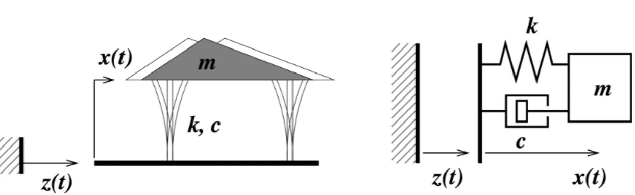
The simplest representation of the dynamic behavior of a building is a single degree of free-dom (SDOF) oscillator. It consists of a spring-mass-damper system where the lumped mass moves in only one direction. Such model is specially convenient to reproduce the horizontal vibrations of a single-story building (Figure 2.1).

The dynamic equilibrium is obtained by balancing the inertia, damping and elastic forces, fI, fDand fS, respectively

fI+ fD+ fS= f (t ) (2.1)

fI= m ¨u(t ) (2.2)

fD= c ˙u(t ) (2.3)

fS= ku(t ) (2.4)

with the external excitation force f (t ), where u(t ) is the displacement of the center of mass of the moving object, m is the mass of the moving object, c is the linear viscous damping coefficient and k is the linear elastic stiffness.

The following equation of motion is obtained by substitution of expressions 2.2, 2.3 and 2.4 in 8

2.1. Structural dynamics

Figure 2.2 – Representation of a single degree of freedom oscillator subjected to ground motion (from Gavin, 2014).

equation 2.1:

m ¨u (t ) + c ˙u (t ) + ku (t) = f (t) (2.5)

The principal concern for structural engineers in earthquake prone regions is the behavior under seismic induced motion at the base of the structure (Figure 2.2). The solicitation on the structure is caused by the inertial force to resist the ground acceleration ¨ug(t )

f (t ) = −m ¨ug(t ) (2.6)

Referring to equation 2.6, the equation of motion 2.5 may be rewritten as

m ¨u (t ) + c ˙u (t ) + ku (t) = −m ¨ug(t ) (2.7)

2.1.2 Free vibration

Free vibration is characterised by a null external excitation f (t ), where the disturbance is initiated by an imposed initial displacement d0and velocity v0to the mass. By imposing such

conditions, equation 2.5 is modified as

m ¨u (t ) + c ˙u (t ) + ku (t) = 0 (2.8)

d0= u(0) (2.9)

Undamped vibration

In the undamped case, for c = 0, the response is an oscillation, u(t), of given amplitude and frequency, which can be described by sinusoidal functions. The differential equation governing the free vibration of undamped systems corresponds to

m ¨u (t ) + ku (t) = 0 (2.11)

the solution of this homogeneous differential equation 2.11 taking into account the initial conditions 2.9 and 2.10 is a simple harmonic motion in the form

u(t ) = d0cos(ωnt ) + v0

ωn

sin(ωnt ) (2.12)

whereωnis the natural angular frequency of the system

ωn=

p

k/m (2.13)

Note thatωnhas units of radians per second and is independent of the initial conditions or

external solicitations. The time required to complete an oscillation cycle, Tnis called natural period of the system, measured in seconds, and is related toωn. The natural cyclic frequency

of the system, fn, measured in Hertz, represents the number of cycles executed in one second

fn=

1 Tn =

ωn

2π (2.14)

Viscously damped vibration

In the general case of damped systems the dynamic response decays with time. The simplest representation of such decrement is the linear viscous damping, proportional to the velocity (see equation 2.3). A division of the dynamic equilibrium equation 2.8 by the mass, m, gives

¨

u (t ) + 2ξωnu (t ) + ω˙ 2nu (t ) = 0 (2.15)

2.1. Structural dynamics

whereξ is the, dimensionless damping ratio

ξ = c

2mωn = c cr

(2.16)

where ccris the critical damping coefficient

ccr= 2mωn= 2

p

km = k

ωn

(2.17)

Note that the damping coefficient c is a measure of the dissipated energy during a cycle of forced harmonic vibration, while the damping ratioξ is a property of the system dependent of its mass and stiffness.

The form of the solution of equation 2.15, corresponding to the response of the structure, is dependent of the amount of damping present in the system. The types of motion, caused by an initial displacement x0, are classified as (see Figure 2.3):

• Undamped : if c = 0 or ξ = 0, the system response does not decay.

• Critically damped : if c = ccr orξ = 1, the system returns to equilibrium without

oscillat-ing.

• Overdamped : c > ccrorξ > 1, the system returns to equilibrium without oscillating and

with a slower rate than in the critically damped situation.

• Underdamped : 0 < c < ccr or 0 < ξ < 1, the system oscillates decreasing its amplitude

around the equilibrium position.

Civil engineering structures (such as buildings, bridges, nuclear power plants, dams, etc.) have typically damping ratios lower than 0.1 (Chopra, 2012). Hence, only the underdamped situation is treated on this manuscript.

The solution of equation 2.15 for underdamped systems, taking into account the initial condi-tions 2.9 and 2.10, is

u(t ) = exp(−ξωDt )(d0cosωDt ) +

v0+ ξωDt ωD

Figure 2.3 – Free vibration of underdamped (ξ < 1), critically damped (ξ = 1) and overdamped (ξ > 1) systems (from Chopra, 2012).

whereωDcorresponds to the damped angular frequency of vibration

ωD= ωn

q

1 − ξ2 _(2.19)

2.1.3 Harmonic excitation

The system is subject to a sinusoidal force of the form p(t ) = p0sin(ωt), where p0 is the

amplitude andω is the exciting frequency. The dynamic equilibrium equation governing the movement is

m ¨u (t ) + c ˙u (t ) + ku (t) = p0sin(ωt) (2.20)

The solution is in the form

up(t ) = C sin(ωt) + D cos(ωt) (2.21)

where 12

2.1. Structural dynamics

Figure 2.4 – Response of undamped (a) and damped (ξ = 0.05) (b) systems to harmonic force ω/ωn= 0.2, with u(0) = 0 and ˙u(0) = ωnp0/k (from Chopra, 2012).

C =p0 k 1 − (ω/ωn)2 (1 − (ω/ωn)2)2+ (2ξ(ω/ωn)2)2 (2.22) D =p0 k −2ξω/ωn (1 − (ω/ωn)2)2+ (2ξ(ω/ωn)2)2 (2.23)

The solution is composed of a transitory and a steady state part:

u(t ) =

Tr ansi t i ent

z }| {

exp(−ξωnt )(A cosωDt + B sinωDt ) +

St ead y st at e z }| { C sinωt + D cosωt (2.24) where A = d0 (2.25) B = v0 ωn− p0 k ω/ωn 1 − (ω/ωn)2 (2.26)

The presence of damping reduces the transitory component amplitude across time, tending to the permanent response (Figures 2.4 and 2.5).

When the load frequency corresponds to the natural frequency of the systemω = ωn, the

sys-tem enters into resonance. Each cycle of excitation is in phase with the structure displacement, increasing the response. The amplitude of the steady-state deformation and the rate at which such state is attained are strongly dependent of damping. In the ideal case of an undamped structure, the deformation amplitude would grow indefinitely with time (Figure 2.5).

Figure 2.5 – Response of undamped (a) and damped (ξ = 0.05) (b) systems to sinusoidal force of frequencyω = ωn, with u(0) = 0 and ˙u(0) = 0 (from Chopra, 2012).

The steady-state deformation caused by an harmonic force can be expressed as

u(t ) = u0sin(ωt − φ) = (ust)0Rdsin(ωt − φ) (2.27)

where u0=

p

C2_{+ D}2_{andφ = tan}−1_{(−D/C ). The deformation response factor, R}

d, is the ratio

of the dynamic deformation amplitude , u0, to the static deformation (ust)0. It determines the

amplification between dynamic and static response and phase angle,φ , that gives the time lag between the excitation and the response are identified as

Rd= u0 (ust)0= 1 p (1 − (ω/ωn)2)2+ (2ξ(ω/ωn))2 (2.28) φ = tan−1µ 2ξ(ω/ωn) 1 − (ω/ωn)2 ¶ (2.29)

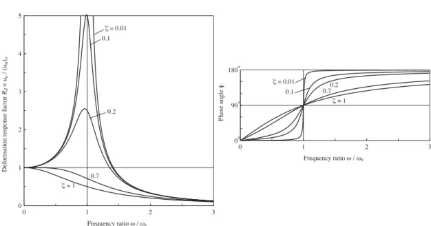
The variation of the deformation amplification and phase angle versus frequency ratioω/ωn,

for different values of damping, is shown in Figure 2.6. The following behaviors are highlighted:

• Ifω/ωn<< 1: the phase angle is close to 0o, hence the displacement is in phase with the

applied force and amplification Rdis slightly larger that 1.

• Ifω/ωn>> 1 the phase angle is close to 180o, hence the displacement is out phase with

the applied force and the amplification Rdtends to zero.

• Ifω/ωn≈ 1 the phase angle is close to 90o, hence the forcing frequency is close to the

resonant frequency of the system and the amplification Rdis very sensitive to damping.

For small values of damping the dynamic response can be much larger than the static deformation.

2.1. Structural dynamics

Figure 2.6 – Deformation response factor and phase angle for a damped system excited by harmonic force (from Chopra, 2012).

In the caseω = ωnthe response is controlled by the damping properties of the system, and

equation 2.27 results in u0= (ust)0/(2ξ). Note that Rd is also referred to as quality factor, Q,

in the literature (Knopoff, 1964). The civil engineering community usually refers to damping ratioξ, while geophysicists to Q, beeing the relationship between both

Q = 1/(2ξ) (2.30)

2.1.4 Seismic response

The time variation of ground acceleration ¨ug(t ) is the most usual representation of the

earth-quake shaking in civil engineering. The first strong motion accelerogram was recorded in 1933, during the Long Beach earthquake (Chopra, 2012). Figure 2.7 shows the acceleration recorded during different significant earthquakes of the XX century. Real earthquakes are far from being sinusoidal mono-frequencial signals. As seen in Figure 2.7, the ground motion varies with time in a highly irregular manner and the earthquake signature can be very different depending of their nature (signal length, amplitude, strong motion duration, etc.).

The equation of motion of a SDOF system subject to ground motion is expressed as

¨

Figure 2.7 – Ground motions recorded during several earthquakes (from Chopra, 2012).

2.1. Structural dynamics

According to equation 2.31, different SDOF systems with identical natural frequency,ωn, and

damping ratio,ξ, sollicited by the same ground motion have the same dynamic behavior, even though they have different masses or rigidity.

The analytical solution of the equation of motion of a system under seismic loading is known at each time instant. Starting from at-rest condition, u(0) = 0 and ˙u(0) = 0, the SDOF deformation time history, u(t ) is obtained as

yk= θ(∆t )yk−1+ γ0(∆t)vFk−1+ γ1(∆t)vFk (2.32)

˙yk= Dyk+ vFk (2.33)

where the subscript k is the iteration step and

yk=   u(tk) ˙ u(tk)   (2.34) θ(∆t) =   −ω2ng (∆t) h(∆t) −ω2nh(∆t) ˙h(∆t)   (2.35) D =   0 1 −ω2n −2ξωn   (2.36) γ0(∆t) = µ θ(∆t) − 1 ∆tL(∆t) ¶ D−1 (2.37) γ1(∆t) = µ ₁ ∆tL(∆t) − I ¶ D−1 (2.38) L(∆t) = (θ(∆t) − I)D−1 (2.39) v =h0 1 iT (2.40)

Figure 2.8 – One degree of freedom base model for: (a) system on a elastic soil, (b) discrete system where base compliance is represented by springs and dashpots, (c) components of motion of base and mass (from Kramer, 1996).

g (∆t) = − 1 ω2 n e−ξωn∆t µ cos(ωD∆t) +ξωn ωD si n(ωD∆t) ¶ (2.41) h(∆t) = ˙g(∆t) = 1 ωD e−ξωn∆t_{si n(}ω D∆t) (2.42) ˙ h(∆t) = e−ξωn∆t µ cos(ωD∆t) −ξωn ωD si n(ωD∆t) ¶ (2.43)

whereωDis defined in 2.19. Matrices in equations 2.32 and 2.33 are constant during the time

history.

2.1.5 Effects of SSI on natural frequencies

To illustrate the most important effects of soil-structure interaction, the case of a SDOF system mounted on a rigid, massless, L-shape foundation supported on an elastic soil (Figure 2.8a) is adopted (Wolf, 1985). Being the structure characterized by its mass, m, stiffness, k, and damping coefficient c, the fixed-base natural frequency,ωn, and hysteretic damping ratio,ξ,

are, respectively (as described in Section 2.1.2):

ωn=

p

k/m (2.44)

ξ =cωn

2k (2.45)

However, if the supporting material is compliant with the structure, the foundation can rotate and translate. The compliant soil-foundation system is shown in Figure 2.8b, where stiffness 18

2.1. Structural dynamics

and damping characteristics are represented by springs and dashpots. Two sources of damping are represented: material damping (caused by the inelastic behavior of the foundation) and radiation damping (caused by the soil deformation due to dynamic forces in the structure). Radiation damping is often much greater than material damping for typical foundations (Kramer, 1996). The total displacement of the base and the structural mass can be separated in individual components (see Figure 2.8b). Then, the natural frequency of the equivalent model, ωe, can be obtained as a combination of: the natural frequency of the fixed-base system,ωn,

the natural frequency for translational vibration,ωhand the natural frequency for rocking,ωr.

1 ω2 e = 1 ω2 n + 1 ω2 h + 1 ω2 r (2.46) ωe=p ωn 1 + k/kh+ kh2/kr (2.47)

Equation 2.47 shows that the natural frequency of a system considering soil-structure in-teraction always decreases with respect to the fixed-base structure. Hence, the greater the importance of the soil-structure interaction, the greater the reduction of the natural frequency.

2.1.6 MDOF systems

Modal analysis

Vibrational approach for the estimation of seismic response of multi-degree-of-freedom (MDOF) systems in earthquake engineering comes from the general theory of transitient response by Biot (1932).

The dynamic response of a structure can be represented by a SDOF model in the case of one story buildings or structures with a single lumped mass at their head (water towers, airport control towers, etc.).

The equation 2.7 for structures with MDOF becomes

The modal transformation

u = Φq (2.49)

is adopted to diagonalize the matrices in equation 2.48.Φ is the modal matrix, which columns are the eigenvectors obtained solving the following eigenproblem 2.50:

KΦ = MΦΩ2 (2.50)

Imposing the condition

|K − λM| = 0 (2.51)

the eigenvaluesλi can be deduced, with i = 1,...,n, where n is the number of degrees of

freedom of the MDOF system. They correspond to the squared angular frequenciesω2_i of the structure, withω1< ω2< ... < ωn. If the modal matrix is orthonormal with respect to the mass

matrix M, equation 2.48 becomes

¨

q(t ) + Ξ˙q(t) + Ω2q(t ) = −ΦTMτ ¨ug(t ) (2.52)

whereΞ = di ag{2ξωi} andΩ2= di ag {ω2_i}. Thanks to modal transformation 2.52 is a system

of independent equations where each one is the dynamic equilibrium equation of a SDOF system, which analytical solution is known at each time step.

Once evaluated the modal displacement vector q, the modal transformation 2.49 provides nodal displacement vector u of the MDOF system. The same relationship is adopted for velocity and acceleration

˙

u = Φ˙q (2.53)

¨

u = Φ¨q (2.54)

This procedure avoids numerical time integration schemes and reduces computational time.

2.1. Structural dynamics

Modal transformation is possible according to the superposition principle and is only valid for linear behavior of materials.

Further works facilitate the application of the theory (Biot, 1933, 1934) introducing the actually known as response spectrum method. Nowadays, such approach is commonly used by earthquake engineers after 80 years without many changes (Trifunac, 2008a). The response spectrum method proposes to use the maximum expected acceleration for the analyzed seismic zone (depending on the building period) instead of a reference acceleration time-history.

Direct integration dynamic analysis

The differential equation 2.48 can be directly solved using an implicit algorithm as a Newmark process. It can be written in incremental form as

M∆¨uk+ C∆ ˙uk+ K∆uk= −Mτ∆ ¨ug k= ∆Fk (2.55)

where uk= u(tk). The solution is obtained by defining displacement and velocity as function

of acceleration, according to the following expressions:

˙

u_k+1= ˙uk+ (1 − γ)∆t ¨uk+ γ∆t ¨uk+1 (2.56)

u_k+1= uk+ (∆t ) ˙uk+ (0.5 − β)(∆t )2u¨k+ β(∆t )2u¨k+1 (2.57)

Parametersβ and γ define the variation of acceleration over a time step, characterising the accuracy and stability of the method. If they are assumed according to 2β ≥ γ ≥ 1/2, uncondi-tional stability of the method is assured.

Hilbert, Hughes and Taylor (Hughes, 1987) introduce theα-method as improvement of New-mark process. The time discrete equation of motion is modifies as follows:

M∆¨u_k+1+(1+α)C∆ ˙uk+1−αC∆ ˙uk+(1+α)K∆uk+1−αK∆uk= (1+α)∆Fk−α∆Fk−1 (2.58)

Ifα = 0 equation 2.58 reduces to the Newmark method. If the parameters are selected such thatα ∈ [−1/3,0], γ = (1 − 2α)/2, and β = (1 − α)2/4, an unconditionally stable, second-order

accurate scheme results. Atα = 0, the trapezoidal rule is obtained. Decreasing α increases the amount of numerical dissipation.

The damping matrix in equation 2.48 can be assumed dependent on mass and stiffness matrices, and expressed according to the Rayleigh approach

Ck= aM + bKk (2.59)

The coefficients are estimated as function of the first and second natural angular frequencyω1

andω2, respectively: a = 2ξ ω1ω2 ω1+ ω2 (2.60) b = 2ξ 1 ω1+ ω2 (2.61) 2.1.7 Euler–Bernoulli beam

Structures with one predominant dimension in relation to the other two can be modeled as beam elements with rigidity and mass homogeneously distributed along the element axis. The Euler–Bernoulli beam theory (Timoshenko, 1953) describes the behavior of a beam under bending deformation under the assumption of negligible axial and shear strain. Consequently, the beam cross-section remains orthogonal to the beam axis during deformation. The beam movement is described by the following equation (Clough and Penzien, 2003):

∂4_{u(x, t )} ∂x4 + m E I ∂2_{u(x, t )} ∂t2 = 0 (2.62)

where u(x, t ) is the displacement, m is the mass, E is the elasticity modulus in compression and I is the moment of inertia. The solution of the differential equation 2.62 is achieved by modal decomposition of time, t , and space, x, variables:

u(x, t ) = φ(x)U (t) (2.63)

whereφ(x) is function of the modal shape and U(t) represents the amplitude for a given time. By applying the decomposition, equation 2.62 results:

2.1. Structural dynamics ∂2_{U (t )} ∂t2 + ω 2 0U (t ) = 0 (2.64) ∂4_φ(x) ∂x4 + α 4_{φ(x) = 0 (2.65)}

whereα4 = (mω20)/(E I ) and ω0 is the fundamental angular frequency of the beam. The

solutions of equations 2.64 and 2.65 are respectively:

U (t ) = A cos(ω0t ) + B sin(ω0t ) (2.66)

φ(x) = C1sin(αx) +C2cos(αx) +C3sinh(αx) +C4cosh(αx) (2.67)

where A and B are constants related to the initial displacement, U0, and velocity, V0. Constants

C 1, C 2, C 3 and C 4 are related to the boundary conditions of the beam. For the specific case of a cantilever beam (fixed at the base and free at the top), rotations and displacements are null at the base, while shear, V , and moment, M , are null at the top:

u(0, t ) = 0 → φ(0) = 0 → C 4 = −C 2 (2.68) ∂u(t) ∂x = 0 → ∂φ(0) ∂x = 0 → C 3 = −C 1 (2.69) M (H , t ) = 0 → E I∂ 2_φ(H) ∂2_x = 0 →

C 1(sin(αH) + sinh(αH)) +C2(cos(αH) + cosh(αH)) = 0 (2.70)

Q(H , t ) = 0 → E I∂

3_φ(H)

∂3_x = 0 →

C 1(cos(αH) + cosh(αH)) +C2(−sin(αH) + sinh(αH)) = 0 (2.71)

The solutions of the system can be obtained numerically trough the following equation:

1 + cos(αH)cosh(αH) = 0 (2.72)

f1= 0.5596 H2 s E I m (2.73) fn f1 = 0.7(2n − 1) 2 ∀n > 1 (2.74)

which leads to frequencies ratios characteristics of a beam with bending behavior: f2/ f1= 6.3,

f3/ f1= 17.5, f4/ f1= 34.3, etc.

2.1.8 Timoshenko beam

Timoshenko beam theory (Timoshenko, 1921, 1922) considers a non negligible shear strain of the beam under shear effort. Consequently, orthogonality of the beam cross-section to the beam axis is not imposed, as in the Euler-Bernoulli beam theory. The difference between both, Euler-Bernoulli and Timoshenko, beam theories lies on their assumptions. The contribution of shear strain leads to the equation of motion (Dunand, 2005)

∂2_{u(x, t )} ∂x2 + m GS ∂2_{u(x, t )} ∂t2 = 0 (2.75)

where S is the cross section area and G is the shear modulus. Equation 2.75, using modal decomposition (equation 2.63), becomes

∂2_{U (t )} ∂t2 + ω 2 0U (t ) = 0 (2.76) ∂2_φ(x) ∂x2 + α 2_{φ(x) = 0 (2.77)}

whereα2= (mω2₀)/(GS) andω0 is the fundamental angular frequency of the beam. The

solutions of equations 2.76 and 2.77 are respectively

U (t ) = A cos(ω0t ) + B sin(ω0t ) (2.78)

φ(x) = C1cos(αx) +C2sin(αx) (2.79)

where A and B are constants related to the initial displacement, U0, and velocity, V0. C 1 and

C 2 are related to the boundary conditions of the beam. For the case of a cantilever beam:

2.1. Structural dynamics

u(0, t ) = 0 → φ(0) = 0 → C 1 = 0 (2.80)

Q(H , t ) = 0 → cosh(αH) = 0 (2.81)

The natural frequencies can be obtained from the solutions of equation 2.81:

fn=n − 0.5 2H s GS m (2.82) fn f1 = (2n − 1) ∀n > 1 (2.83)

which leads to the frequency ratios that are characteristics of a beam with not negligible shear strain: f2/ f1= 3, f3/ f1= 5, f4/ f1= 7, etc.

The equation defining the movement in the modal base (after variable separation of equation 2.63) is (Hans, 2002) E I∂ 4_φ(x) ∂x4 + E I K mω 2∂2φ(x) ∂x2 − mω 2_{φ(x) = 0} (2.84)

where K is a shear parameter according to V (x) = −K γ(x), where γ is the shear strain and V the associated shear force. The behavior of an Euler-Bernouilli beam is stiffer than a Timoshenko beam, in the case of slender enough structures the error for both models is relatively small. In the case of structures with smaller length to thickness ratios, the Timoshenko beam is a more appropriate choice (as shear effects are more relevant).

A beam with predominant bending behavior is sometimes referred as bending beam, and to a beam with predominant shear behavior as shear beam. A dimensionless parameter of a beam (Michel, 2007)

C = E Iπ

2

4K H2 (2.85)

related to the structural behavior, is useful to inform if the bending type behavior is predom-inant or rather the shear one. A structure is considered to behave in bending for values of C < 0.05, and in shear for values of C > 5 (Boutin et al., 2005). Figure 2.9 shows the variation of frequency ratios with the parameter C , it is observed that the case values of pure bending

Figure 2.9 – Variation of frequency ratios fn/ f1for modes above the fundamental frequency

with the dimensionless parameter C , for a continuous Timoshenko beam. Grey areas represent the limit for bending and shear beam behavior (Michel, 2007).

beam are found for C → 0, while pure shear are found for C → ∞.

Additional details about Timoshenko beam theory are discussed in Section 6.3.2

2.2 Instrumentation of buildings

2.2.1 Vibrational analysis of buildings

Recordings of vibrations in civil engineering structures are undertaken at the beginning of the XX century by the seismologist Fusakichi Omori in Japan. He records earthquakes on masonry between 1900 and 1908, with the aim to observe structures to increase seismic resistance (Davison, 1924). Omori takes records during the construction of buildings, after seismic damage and after rehabilitation (Omori, 1922). After him, researchers in Japon (Ishimoto and Takahasi, 1929) and the United States (Byerly et al., 1931) continued to further investigate this topic.

The earthquakes of Santa Barbara in 1925 (6.8 magnitude, 13 deaths and 8$ millions in dam-ages) and Long Beach in 1933 (6.4 magnitude, 115 deaths and 40$ millions in damdam-ages) encouraged the implementation of the program US Coast and Geodetic Survey. Leaded by Dean Carder, 336 buildings were instrumented and their fundamental periods were obtained. The study establishes the first empirical relationship between building height and period (Carder, 1936), which settles the principles afterward used in the para-seismic codes (Housner and Brady, 1963).