Depth dependence of westward-propagating North Atlantic features diagnosed from altimetry and a numerical 1/6° model

(1)

HAL Id: hal-00331135

https://hal.archives-ouvertes.fr/hal-00331135

Submitted on 12 Nov 2007

HAL is a multi-disciplinary open access

archive for the deposit and dissemination of sci-entific research documents, whether they are pub-lished or not. The documents may come from teaching and research institutions in France or abroad, or from public or private research centers.

L’archive ouverte pluridisciplinaire HAL, est destinée au dépôt et à la diffusion de documents scientifiques de niveau recherche, publiés ou non, émanant des établissements d’enseignement et de recherche français ou étrangers, des laboratoires publics ou privés.

Depth dependence of westward-propagating North

Atlantic features diagnosed from altimetry and a

numerical 1/6° model

Albanne Lecointre, Thierry Penduff, P. Cipollini, R. Tailleux, Bernard Barnier

To cite this version:

Albanne Lecointre, Thierry Penduff, P. Cipollini, R. Tailleux, Bernard Barnier. Depth dependence of westward-propagating North Atlantic features diagnosed from altimetry and a numerical 1/6° model. Ocean Science Discussions, European Geosciences Union, 2007, 4 (6), pp.817-853. �hal-00331135�

(2)

OSD

4, 817–853, 2007 3-D investigation of Rossby waves A. Lecointre et al. Title Page Abstract Introduction Conclusions References Tables Figures ◭ ◮ ◭ ◮ Back Close

Full Screen / Esc

Printer-friendly Version Interactive Discussion

EGU

Ocean Sci. Discuss., 4, 817–853, 2007 www.ocean-sci-discuss.net/4/817/2007/ © Author(s) 2007. This work is licensed under a Creative Commons License.

Ocean Science Discussions

Papers published in Ocean Science Discussions are under open-access review for the journal Ocean Science

Depth dependence of

westward-propagating North Atlantic

features diagnosed from altimetry and a

numerical 1/6

◦

model

A. Lecointre1, T. Penduff1, P. Cipollini2, R. Tailleux3, and B. Barnier1 1

Lab. des Ecoulements G ´eophysiques et Industriels, CNRS, UJF, INPG, Grenoble, France

2

National Oceanography Centre, Southampton, UK

3

Department of Meteorology, University of Reading, UK

Received: 23 October 2007 – Accepted: 29 October 2007 – Published: 12 November 2007 Correspondence to: A. Lecointre (Albanne.Lecointre@hmg.inpg.fr)

(3)

OSD

Full Screen / Esc

EGU

Abstract

A 1/6◦ numerical simulation is used to investigate the vertical structure of westward propagation between 1993 and 2000 in the North Atlantic ocean. The realism of the simulated westward propagating signals, interpreted principally as the signature of first-mode baroclinic Rossby waves (RW), is first assessed by comparing the

sim-5

ulated amplitude and zonal phase speeds of Sea Level Anomalies (SLA) against TOPEX/Poseidon-ERS satellite altimeter data. Then, the (unobserved) subsurface sig-nature of RW phase speeds is investigated from model outputs by means of the Radon Transform which was specifically adapted to focus on first-mode baroclinic RW. The analysis is performed on observed and simulated SLA and along 9 simulated

isopyc-10

nal displacements spanning the 0–3250 m depth range. Simulated RW phase speeds agree well with their observed counterparts at the surface, although with a slight slow bias. Below the surface, the simulated phase speeds exhibit a systematic deceleration with increasing depth, by a factor that appears to vary geographically. Thus, while the reduction factor is about 15–18% on average at 3250 m over the region considered, it

15

appears to be much weaker (about 5–8%) in the eddy-active Azores Current, where westward propagating structures might be more coherent in the vertical. These results suggest that the often-made normal-mode assumption of many WKB-based extended theories that the phase speed is independent of depth might need to be revisited. They also suggest that the vertical structure of westward propagating signals could

signif-20

icantly depend on their degree of nonlinearity, with the degree of vertical coherence possibly increasing with the degree of nonlinearity.

1 Introduction

Rossby or planetary waves (Rossby, 1939), discussed for the first time by Hough

(1897) are instrumental in the western intensification of oceanic gyres (Anderson and 25

(4)

OSD

Full Screen / Esc

EGU

(Pedlosky,1979;Gill,1982), and possibly in the variability of the Meridional Overturning

Circulation (MOC) (Hirschi et al.,2006). Until recently, the main theoretical framework to describe such waves has been the standard linear theory (referred to as SLT there-after), which is based on quasi-geostrophic (QG) assumptions and a decomposition of oceanic motions on a discrete basis of normal mode solutions (Gill,1982). These

5

include a very fast barotropic mode whose associated horizontal velocity profile is in-dependent of depth, and an infinite number of baroclinic modes of increasing vertical complexity. The appealing simplicity of the SLT has made it a widely used interpre-tative tool by oceanographers, even though its validity, relevance, and accuracy have never been really tested owing to the traditional difficulty of sampling the oceans at the

10

temporal and spatial scales pertaining to planetary wave propagation.

Over the last decade, however, the advent of satellite altimetry has rapidly lead to improving our knowledge of the empirical properties of planetary wave propagation by providing global observations of the surface signature of these waves with unprece-dented spatial and temporal resolutions. So far, although limited to the surface, such

15

observations have already proved sufficient to question the validity of the SLT on a number of points. Specifically,Chelton and Schlax(1996) showed that observed phase speeds appear to be two to three time faster at mid- and high-latitudes than predicted by the SLT; furthermore, the observed wave amplitude do not appear to remain uniform throughout ocean basins as anticipated by the SLT, but to have enhanced variance in

20

the western part of the basins.

Chelton and Schlax(1996)’s results greatly stimulated the development of new

theo-ries seeking to improve upon the SLT by taking into account such neglected effects as the background mean flow, topography, and nonlinearities, to cite the most important ones. Early theories focused on non-dispersive long waves, and initially focused on

25

the effects of a background zonal mean flow over a flat-topography as the most likely explanation to account for the discrepancy, e.g.,Killworth et al.(1997). The effect of topography was initially discarded byKillworth and Blundell(1999) as being relevant,

(5)

OSD

Full Screen / Esc

EGU

if properly considered, can have a much greater impact than the background mean flow on Rossby wave phase speeds, see alsoTailleux(2003,2006) for a further discussion of the topographic effects. Over the past few years, the increase in spatial resolution of satellite altimeter products achieved by merging different altimeter datasets motivated the study of the empirical dispersion relation of Rossby waves. This in turn prompted

5

the most recent theories to include dispersive effects as well. The most complete the-ory to date is probably that ofKillworth and Blundell(2005) which considers the effects of dispersion and background mean flow in presence of a variable large-scale topogra-phy, in the context of WKB theory.

While the extended theories appear to do better than the SLT at reducing the

dis-10

crepancy with observations, e.g.,Maharaj et al.(2007), this does not necessarily mean that they do so for the correct reasons. This is because the extended theories, despite their apparent success, still rely on a number of assumptions whose validity can nei-ther be directly checked against observations, nor rigorously proven mathematically. Indeed, such theories are for the most part based on the WKB approximation whose

15

validity relies in principle on a scale separation between the waves and the medium of propagation, as well as on the non-interaction between the different waves sup-ported by the system. While the idea of a scale separation between the waves and the background large-scale circulation does not appear unreasonable at leading order, it seems much more questionable with respect to addressing the effects of

topogra-20

phy since the latter exhibits important variations on both small and large scales. The latter issue is not easily dismissed, because the studies byKillworth et al. (1997) and

Tailleux and McWilliams(2001) show that the bottom boundary condition have a much

greater impact that the background mean flow on the phase speed when both effects are considered separately. With regard to the non-interaction assumption underlying

25

WKB theory,Tailleux and McWilliams(2002) andTailleux(2004) suggest that it breaks down in places where the topography has a strong curvature, which is likely to occur widely in the actual ocean.

(6)

plan-OSD

Full Screen / Esc

EGU

etary waves are able to retain a normal mode structure similar to that of the standard modes, despite the linearised equations in presence of background mean flow and topography being no longer separable. As a result, these extended theories assume that the propagation remains vertically coherent, as for standard normal modes, with the implication that westward propagation should be observable throughout the

verti-5

cal with a phase speed independent of depth. Of course, such a particular prediction is difficult to test against observations, although this might become feasible in the fu-ture using ARGO floats, as initiated byChu et al. (2007). From a physical viewpoint, the validity of the normal mode assumption is not obvious. Indeed, vertical normal modes are usually interpreted as a standing wave resulting from the superposition of

10

two modes propagating vertically in opposite directions, with the same amplitude but opposed phase speeds. As a result, the persistence of normal modes requires: 1) that the problem be symmetric with respect to upward and downward propagation; 2) that the amplitude of the reflected waves at the bottom and surface boundaries be the same as that of the incident waves. Obviously, this is technically not true for the linearised

15

equations in presence of a background mean flow and bottom topography, so that the degree to which planetary waves can be regarded to be associated with normal modes should probably be more fully justified than has been the case so far. An alternative is to look at the 3-D propagation of planetary wave packets, as proposed byYang (2000), but then additional difficulties arise with respect to how to satisfy boundary conditions,

20

while the other difficulties associated with the scale-separation and non-interaction re-main.

Finally, the last difficulty in interpreting actual planetary wave propagation stems from the possibility that a large fraction of observed westward propagating signals could actually be associated with nonlinear eddies, rather than with linear waves, as recently

25

pointed out byChelton et al. (2007). That nonlinearities are likely to be important for the study of westward propagating signals is in fact theoretically motivated by the study

ofJones(1979) who was the first to demonstrate that linear Rossby waves are always

(7)

OSD

Full Screen / Esc

EGU

are always unstable, and therefore nonlinear interactions important, the question that naturally arises is how accurate and relevant our linear theories can be?

With so many interrogations about the validity of extended theories, as well as about the linear or nonlinear nature of actual Rossby waves, it appears urgent and desirable to learn more about the full three-dimensional structure of westward propagation in

5

order to make progress toward checking existing theories and possibly proposing sug-gestions for improvement. So-called “realistic” ocean model simulations can fruitfully complement such idealised (analytical or numerical) Rossby wave studies, to inves-tigate the full 3-D (unobserved) structure of the waves. These numerical simulations take into account high resolution topography and geometry, realistic initial state, forcing

10

and stratification to mimic the observed state and evolution of the real ocean, and can thus be directly compared to observations. However, the unambiguous extraction and identification of individual processes and signals is more difficult in such simulations than in idealised models. Hughes (1995) and Hirschi et al. (2006) made use of “re-alistic” numerical simulations to investigate Rossby waves over the Southern Ocean

15

surface, and the role of Rossby waves in the variability of the MOC, respectively. The outputs of the ATL6 1/6◦Clipper realistic model (Penduff et al.,2004) are used here to study the vertical structure of the waves.

The propagation of Rossby waves has a dominant westward component that ap-pears clearly on longitude/time sections (also known as Hovm ¨uller diagrams). In the

20

literature, the two main signal processing techniques that have been used to extract and study surface Rossby waves from such diagrams are the 2-D Radon Transform (RT) and the 2-D Fourier Transform. The RT (Radon,1917;Deans,1983) provides an quantitative estimate of the orientation of lines in Hovm ¨uller plots.Chelton and Schlax

(1996) first used the RT to study the characteristics (especially the phase speed) of

25

westward-propagating planetary waves in satellite altimeter data. Since then, several authors have applied the 2-D RT on SST or SLA datasets (Hill et al., 2000;Maharaj

et al., 2004, 2005; Cipollini et al., 2001, 2006). Superimposed propagating signals locally extracted by the 2-D RT are generally interpreted as various baroclinic modes

(8)

OSD

Full Screen / Esc

EGU

of Rossby waves (Maharaj et al.,2004;Cipollini et al.,2006). The 2-D RT is used in the present study to extract the first baroclinic mode of Rossby waves from observed and simulated data in the subtropical North Atlantic. Some limitations of the 2-D RT are pointed out and this paper explains how the method has been adapted.Challenor et al.

(2001) applied a 3-D RT on altimeter data in the North Atlantic and showed that the

5

meridional phase speed was negligible in many places, thus justifying that only the 2-D RT is used here. Some authors (Subrahmanyam et al.,2000;Osychny and Cornillon,

2004;Maharaj et al.,2007) have used the 2-D Fourier Transform instead of the 2-D RT.

This alternative approach highlights the spectral components of the data in time and space and provides a different estimate of superimposed phase speeds.Maharaj et al. 10

(2004);Cipollini et al.(2006) explored the differences between both methods.

The purpose of this paper is to investigate and describe the vertical (unobserved) structure of westward propagation in the CLIPPER ATL6 model. To that end, we first seek to build our confidence in the physical plausibility of the model results by first assessing the ability of the model to simulate the speed and amplitude of westward

15

propagating as observed by satellite altimetry in the subtropial North Atlantic. The primary method to investigate westward propagation is the 2-D RT applied on simulated isopycnal displacements. The datasets are presented in Sect.2. Section3present how we modified the classical 2-D RT to better select the first baroclinic mode of Rossby waves. Our results are presented in Sect.4, then summarised and discussed in Sect.5.

20

2 Observed and simulated datasets

2.1 Observations

We make use of the merged Topex/Poseidon-ERS Sea-Level Anomaly (SLA) maps distributed by AVISO. SLA fields as a function of (x, y, t) are available weekly over

the world ocean from October 1992 onwards on a 1/3◦ MERCATOR grid. Details the

25

(9)

OSD

Full Screen / Esc

EGU

The reader is also referred to the DUACS handbook (http://www.jason.oceanobs.com/

documents/donnees/duacs/handbook duacs.pdf) and toCLS(2004) for further details. Rossby wave amplitudes are weak and difficult to detect polewards of 50◦N. In the equatorial band, their wavelengths may also become longer than our 20◦analysis win-dow (see Sect.3.1) and get aliased by the RT (Cipollini et al.,2001). This study thus

5

focuses on the subtropical North Atlantic from 5◦N to 50◦N and covers the 8-year pe-riod (from 1993 to 2000) coinciding with the pepe-riod of numerical simulations.

2.2 Simulations

Numerical data come from the ATL6-ERS26 1/6◦simulation (Penduff et al.,2004) per-formed during the French CLIPPER project (Tr ´eguier et al., 1999), a high resolution

10

model study of the Atlantic circulation based on OPA 8.1 numerical code (Madec et al.,

1988). The ATL6 model resolves the primitive equations on an isotropic 1/6◦ MER-CATOR grid spanning the whole Atlantic Ocean (98.5◦W–30◦E, 75◦S–70◦N) with 42 geopotential levels. The model is driven by wind stresses, heat and salt fluxes com-puted from the ECMWF ERA15 reanalysis and subsequent analyses (Barnier,1998).

15

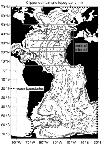
The model is limited by four open boundaries located at 70◦N, in the Gulf of Cadiz (8◦W), at the Drake Passage (68◦W) and between Africa and Antarctica (30◦E). The model topography in the North Atlantic is presented in Fig. 1. The temporal resolution of the numerical dataset is 5 days. Simulated data used in this work are the model

SLA(x, y, t) and the displacements of 9 isopycnals h′(x, y, t) located between 750

20

m and 3250 m. The densities of selected isopycnals areσ1=31.75, 32.05 and 32.25,

σ2=36.9, 36.95 and 36.9875, σ3=41.45, 41.475 and 41.5. Their time-averaged depths over the domain of interest are close to 750, 1000, 1250, 1750, 2000, 2250, 2750, 3000 and 3250 m, respectively, thus yielding a reasonably regular sampling on the ver-tical. The time-space domain used for this study is the same as for the observed data

25

(5◦N–50◦N, 1993–2000).

Figure 2 presents the observed and simulated surface eddy kinetic energy (EKE) in the North Atlantic. The observed EKE is computed over the period October 1992–

(10)

OSD

Full Screen / Esc

EGU

October 2000 from SLA maps by assuming a geostrophic balance (details can be found inDucet et al.,2000). The model EKE is computed for the period 1993–2000 as the velocity variance 1₂((u−u)2+(v−v)2) below the Ekman layer (100 m) to avoid the ageostrophic Ekman components. The path of the main eddy-active fronts is simu-lated correctly by the CLIPPER model in the region of interest. As expected from the

5

relatively modest resolution of the model, the simulated EKE is weaker than in reality. Despite a too zonal North Atlantic Current, the Azores Current is correctly located. This simulation has been compared to various observations and was shown to be realistic in many aspects, including its interannual surface variability (seePenduff et al.,2004

and references therein).

10

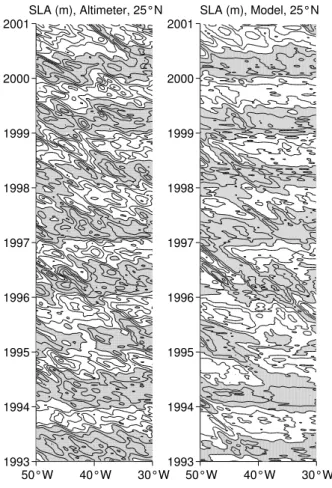
This static view of ocean variability is complemented by longitude-time (Hovm ¨uller) diagrams. These diagrams allow a dynamic view along zonal sections of the data showing the westward propagation of signals as oblique structures (Fig. 3). The slope of these structures is inversely proportional to the phase speed of westward-propagating signals. The longitude-time plots of the 9 simulated isopycnal immersion

15

depths (not shown) exhibit comparable oblique structures, showing the presence of westward-propagating signals at every depth.

3 Data processing

This section presents how westward-propagating features are quantified from Sea Level Anomaly fields (SLA) and simulated isopycnal depths. We modified the

clas-20

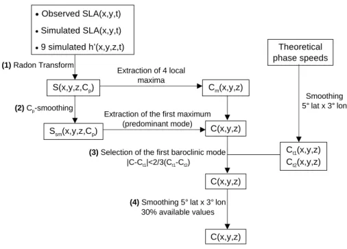
sical Radon Transform algorithm to improve the precision of the analysis, extract first baroclinic mode signals, and regularise resulting phase speed fields. The same pro-cessing technique is applied independently on observed SLAs, simulated SLAs, and on simulated isopycnals. Figure 4 summarises the whole processing.

(11)

OSD

Full Screen / Esc

EGU

3.1 Radon transform

Observed (resp. simulated) SLA timeseries are interpolated linearly on a regular 1/3◦_×1/3◦ (resp. 1/6◦_×1/6◦) horizontal grid, and locally detrended in time over 1993– 2000. Remaining gaps in observed (resp. simulated) fields are filled in the longitude-time space using a 2-D Gaussian interpolation scheme with 1◦_{×7-day (resp. 0.5}◦_×

5

5-day) search radii and 2₃◦_{×1.4-day (resp.} 1₃◦_{×1-day) half-maxima fullwidths.}

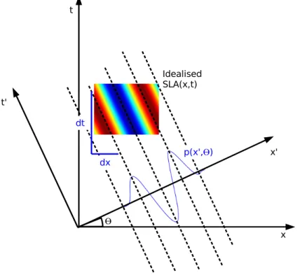
Superimposed zonally-propagating features appear as oblique patterns in longitude-time Hovm ¨uller diagrams. The classical 2-D Radon Transform (RT, described in e.g.

Hill et al.,2000) projects such diagrams from the Cartesian (x,t) plane onto polar

co-ordinates (with the origin at the center of the diagram) as shown in Fig. 5. The RT

10

thus transforms superimposed westward-propagating signals (distinct oblique lines in x,t plane) into vertical stripes parallel to thex′ axis at distinctθ angles. The standard

deviation of the RT (notedS(θ) hereafter) is then computed along the x′axis at every angleθ.

S and subsequent phase speeds are computed throughout the North Atlantic on a 15

1◦_×1◦ grid by applying the Radon Transform on sliding Hovm ¨uller diagrams defined locally. These local diagrams are 20◦ wide in longitude, 8-year tall, extracted at the latitude and centered on the longitude under consideration. Two treatments are per-formed just before applying the RT: the (x,t)-averaged SLA is removed from each local diagram to avoid potential biases in the angle estimate (De La Rosa et al.,2007), and

20

a westward-only filter is applied in the Fourier space to remove eastward-propagating and stationary signals.

3.2 Link between discreteθ angles and phase speeds

The RT projects local Hovm ¨uller diagrams (with dx and d t denoting the zonal and

temporal grid discretisation) along oblique lines whose angles with respect to the

25

vertical span discrete θ values. To each angle θ corresponds the phase speed Cp=(dx/d t) tan θ, with d t usually fixed and dx varying with the cosine of latitude,

(12)

OSD

Full Screen / Esc

EGU

so thatC_p=A cos λ tan θ, with A a constant.

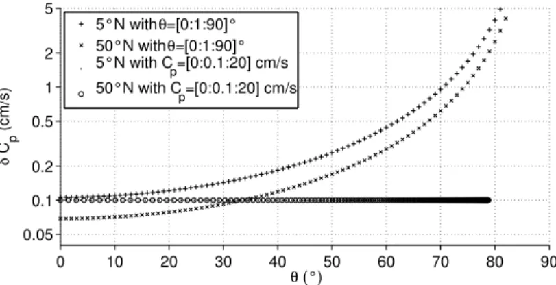
So far, most RT implementations, e.g.,Hill et al.(2000), have used a uniform discreti-sation forθ. However, because of the nonlinear relation between Cpandθ, this implies

a highly non-uniform distribution for the discretisedC_p, which may impair an accurate determination of the phase speeds. Indeed, crosses and pluses in Fig. 6 show that in

5

that case,δCpwould vary by up to a factor of 50 over the range 0–20 cm s−1(θ between

0 and about 80◦). For this reason, we found it preferable to modify the discretisation

ofθ to yield a uniform discretisation of Cp. In the end, the interval 0−20 cm s−1 was

split in constant 0.1 cm s−1 steps. Model and observed, surface and isopycnal phase speed fields were determined independently using this modified algorithm to ensure a

10

uniform precision throughout the basin and phase speed range.

3.3 Smoothing algorithm – extraction of phase speeds

The standard deviation of these Radon Transforms (notedS(x, y, z, Cp) in the

follow-ing) can then be computed along x’ lines (see Fig. 6) at each geographical location to extract the strongest propagating features.

15

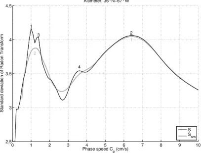
Figure 7 shows a local example ofS(Cp) from altimeter data; local maxima around

6.5 and 1–1.5 cm s−1are close to the expected phase speeds of first and second-mode

Rossby waves, respectively. However, small-scale structures contaminateS(Cp) there,

like in many other locations. This noise affects the automatic detection of significant maxima, and the identification of vertical modes.S fields were smoothed along the C_p 20

axis to avoid such ambiguities. A 11-point boxcar filter was chosen after various tests to remove scales shorter than 1 cm s−1 without affecting meaningful peaks (see thick grey line in Fig. 7). This smoothed field will be notedS_sm(x, y, z, C_p) in the following; it is defined in the range 0.5–19.5 cm s−1 and much less contaminated by small-scale noise.

25

At each (x, y, z), dominant S_sm(C_p) maxima are then found using the following cri-teria: (i) maxima must lie between two increasing and two decreasing values ofSsm;

(13)

OSD

Full Screen / Esc

EGU

(ii) maxima must lie 10 points (1 cm/s) apart from each other. At each location, these maxima yield values ofCm(x, y, z) (m=1, ..., 4), i.e. the phase speeds of the four

dom-inant propagating signals sorted by decreasing amplitude. The same processing has been applied independently to simulated_{S fields at the surface (z=0) and along each} isopycnal.

5

Figure 8 shows zonal and meridional sections of observed and simulated

S_sm(x, y, z=0, Cp) fields (colour), the corresponding dominant phase speed C (white

lines), and the C_m=1−4 fields computed with unsmoothed S (white circles, thick for m=1). The westward and southward acceleration of Rossby waves is realistically

sim-ulated by the model. Intense westward-propagating structures are found in the western

10

basin (a–f) and between 35◦N and 45◦N (a,b,g,h). The 34–36◦N “waveguide” follows the trajectory of the Azores Current, which might contribute to the generation or ampli-fication of the waves (e.g.Cipollini et al.,1999;Cromwell,2006). As expected, theS_sm

maximum (C, white lines) appears less contaminated by small-scale noise than the first

S maximum (C_m=1, open circles), not only in theC_pdirection but also in the horizontal.

15

This beneficial impact is most clearly seen along the western boundary, and between 35◦N and 45◦N.

3.4 Selection of the first baroclinic mode

Several authors have interpreted multiple peaks detected by the 2-D RT as the surface signature of baroclinic Rossby modes (e.g.Subrahmanyam et al.,2000;Maharaj et al.,

20

2004), the strongest signal corresponding to the first mode. Observed and simulated phase speeds are now compared at the surface against extended theory estimates for the first two baroclinic modes (Fig. 8). This theory (Killworth and Blundell,2003) takes into account the effects of a mean baroclinic flow and realistic bathymetry.

These theoretical phase speed fields are noisier than the C field; they were thus 25

smoothed horizontally using a 2-D boxcar filter (cuboid of 5◦in longitude, 3◦in latitude). Resulting fields will be notedCt1 andCt2 hereafter, for the first two baroclinic modes

(14)

OSD

Full Screen / Esc

EGU

speeds C (white lines) correspond very well with C_t1 (white dots) over the domain of interest. Over most of the basin, the distance between observed and simulated phase speeds is also smaller than the distance between C_t1 and C_t2 (not shown): small discrepancies betweenC(altimeter) and C(model) are thus not linked with any

contamination from higher order baroclinic modes.

5

The Radon analysis detects observed and simulated phase speeds (C2,3,4(x, y, z))

in the range of the second baroclinic modeC_t2(white dots). The agreement with theory of these noisy fields is not as good as forCt1, as already mentioned inMaharaj et al.

(2004). LikeMaharaj et al.(2004), we conclude that both the observed and simulated dominant peaks (C) are typical of first baroclinic mode Rossby waves in most regions. 10

Despite the good agreement betweenC and Ct1, there remains a few places where

the first baroclinic mode does not dominate inS_sm (white lines in Fig. 8). We made use ofC_t1andC_t2to remove C values outside the first baroclinic mode range. Cipollini

et al. (2006) already used theoretical speeds to extract the first-mode Rossby wave signals: the strongest peak was saved only if its speed was within 1/3 and 3 times

15

the predicted theoretical first baroclinic mode speed (Killworth and Blundell, 2003), otherwise the second largest peak was selected provided it was within that range. Our sorting algorithm uses theoretical speeds too, but the criteria takes into account

C_t2 to explicitly remove the second baroclinic mode from all the estimations. The C

field is sorted in the following way: at each location (x, y, z), C is conserved only if 20

|C−Ct1|<23(Ct1−Ct2), otherwiseC is masked. Consequently, C is masked where Ct2is not defined (north of the Gulf Stream region). The approach presented above ensures that the phase speeds discussed in the following are close to first baroclinic mode theoretical estimates, and not contaminated by higher-order modes.

3.5 Horizontal smoothing of the phase speed maps

25

Finally, observed and simulatedC(x, y, z) fields were smoothed on the horizontal

inde-pendently (along the 10 levels for the latter) using the 2-D boxcar filter used for theo-retical speeds (5◦×3◦ zonally-elongated cuboids). Smoothed maps are masked where

(15)

OSD

Full Screen / Esc

EGU

less than 30% unsmoothedC(x, y, z) values are available in a cuboid. The amplitude

of the strongest westward-propagating features was computed on the same maps (see AppendixA).

Simulated phase speed fieldsC(x, y, z) are compared with observations at the

sur-face in Sect.4.1; their simulated vertical structure is presented in Sect.4.2.

5

4 Results

4.1 Model/data intercomparison at the surface

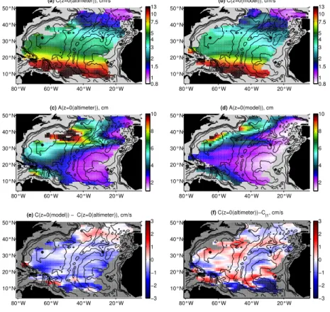
Zones of strong wave amplitudes (Fig. 9c, d) correspond to zones of high EKE (Gulf Stream, Azores current). The simulated Gulf Stream is less energetic than observed and slightly shifted to the north. The similarity of the wave amplitude and EKE fields

10

has already been mentioned byHerrmann and Krauss(1989);Osychny and Cornillon

(2004) in the Gulf Stream region and by Cipollini et al. (1999); Cromwell (2001) at 33◦N and 34◦N. This suggests that most of the eddy activity diagnosed on EKE maps actually propagates to the west.

Simulated surface phase speeds exhibit an slight slow bias, close to 1 cm s−1

15

(Fig. 9e). Model-observation mismatches reach their maximum (i.e. 2 to 3 cm s−1) in the Gulf Stream region, around 10◦N and close to the boundaries of our domain, but become negligible in the Azores Current. As expected from the theory and as shown by several authors (e.g.Tokmakian and Challenor,1993;Polito and Cornillon,1997;

Osychny and Cornillon, 2004), zonal phase speeds increase equatorward and (to a

20

lesser degree) westward (Fig. 9a, b). This feature is well represented by the model, phase speeds reaching 13 cm/s in the southwest part of the domain.

Over most of the basin, the distance between observed and simulated phase speeds is also smaller than the distance betweenC_t1andC_t2(not shown): small discrepancies betweenC(altimeter) and C(model) are thus not linked with any contamination from 25

(16)

OSD

Full Screen / Esc

EGU

As mentioned above, simulated first-mode phase speeds are globally closer to ob-servational than theoretical estimates. Both observed and simulated phase speeds tend to be slower than predicted by the extended theory, except west of the Mid-Atlantic Ridge (MAR) and along 15◦N–20◦N where both are faster (shown in Fig. 9f for the observed phase speeds). This suggests that the impact of bathymetry might be

5

underestimated by the extended theory in this area. 4.2 Vertical structure of first-mode phase speeds

The processing described above has been applied along each of the 9 selected isopy-cnals independently, thus providingC(x, y, z), i.e. a 3-D estimate of the zonal phase

speeds of first mode baroclinic Rossby waves. The ratioC(z)/C(z=0) will be called the 10

Depth-to-surface speed Ratio, noted DR(x, y, z) hereafter. These results might help

complement both (surface restricted) observational studies and theoretical investiga-tions of 3-D Rossby waves (Tailleux,2004,2006).

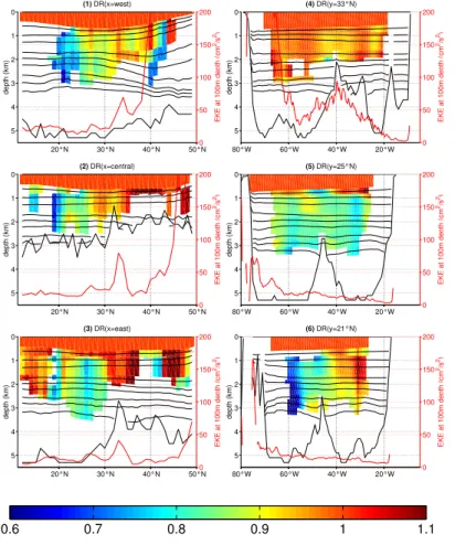
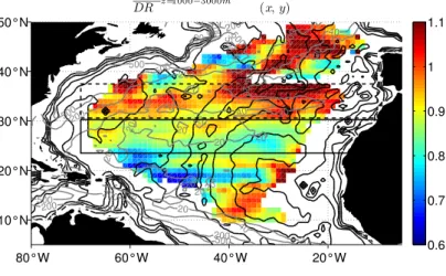
Figures 10, 11, 12 describe the spatial structure of DR(x, y, z) in complementary

ways: along selected sections (Fig. 10); averaged vertically between 1000 and 3000 m

15

(Fig. 11); averaged along isopycnals in two subregions and plotted against the median isopycnal immersion (Fig. 12). Typical values ofDR range between 0.6 and 1.1,

in-dicating the existence of substantial changes in zonal phase speeds with depth. The isopycnal medians ofDR throughout the whole domain (Fig. 11) reveal an overall and

progressive decrease of phase speeds with depth reaching the median value of 15–

20

18% around 3250 m. This basin-scale decrease is very similar to that seen south of the Azores Current (thick black line in Fig. 12). This deceleration occurs around 1000 m, i.e. below the thermocline (right panel is Fig. 12). However, distinct regimes seem to prevail in various regions (Fig. 11).

The downward decrease of phase speeds is similar in the whole basin and in the 24–

25

30◦N band. In this latitude band, however, isopycnal DR distributions are much

nar-rower, suggesting some kind of regional homogeneity. Zonal phase speeds clearly de-crease downward, reaching around 3000 m 75–85% of surface values (Fig. 10 (1,2,5),

(17)

OSD

Full Screen / Esc

EGU

continuous black zone in Fig. 11 and 12). Superimposed on this deceleration pattern, a local influence of the MAR onDR(z) appears along 25◦N (Fig. 10 (5)). DR reaches

a local maximum (0.9) along a line which originates east of the top of the MAR and connects to the surface 1500 km further west. This structure has not been studied in detail, but could illustrate large-scale topographic influences.

5

The situation is different between 31◦N and 37◦N, i.e. around the Azores Current and the southern part of the North Atlantic Current (see Fig. 10 (1–4), dashed black zone in Figs. 11 and 12). The widths ofDR distributions below the thermocline show

that the regimes found within and south of the Azores Front are clearly distinct. Zonal phase speeds vary much less with depth (by about 5%) in this frontal region where

10

mesoscale eddies are more energetic, and where dynamical nonlinearities are en-hanced. Baroclinic energy is transferred into the barotropic mode at eddy scale, pos-sibly enhancing the vertical coherence of oceanic transients in this eddy-active region (where westward-propagating signals are also stronger). One may thus speculate that westward-propagating features in eddy-active areas might be more typical of

vertically-15

coherent eddies than of linear waves, thus moderating the downward deceleration of westward propagation. Further investigations are needed to test this hypothesis.

Figure 12 shows a very significant difference between the range of simulated phase speedsC(z) and the range of theoretical second baroclinic mode phase speeds C_t2

(C(z) being 2.5 to 3 times greater than Ct2). The substantial decrease of phase speeds

20

below the surface does not bring simulated phase speeds close to second-mode esti-mates, but keeps them in the range of first-mode expectations.

North and south of the regions depicted above, results are noisier and more dis-parate (Fig. 10 (6), Fig. 11). At 20◦N–21◦N, the deceleration is weak in the eastern basin and strong in the western basin, with a transition zone above the MAR, where

25

other processes seem to prevail.

It should be mentioned that this downward deceleration of westward phase speeds and its regional patterns are relatively robust and persist in the following cases: (i) no

(18)

OSD

Full Screen / Esc

EGU

of median filters instead of boxcar filters.

5 Discussion – conclusion

The two principal objectives of this work were to evaluate the ability of a realistic high-resolution OGCM to simulate Rossby wave propagation by comparing the simulated and observed surface signatures of such waves, and to document and characterise

5

their (as yet unobserved) vertical structure. The focus was on westward propagating signals whose phase speeds, estimated by means of the Radon Transform, appeared to be close to that anticipated for the first baroclinic mode. The Radon Transform was applied independently on observed and simulatedSLA signals, as well as on 9

simu-lated isopycnal displacements located between 750 m and 3250 m. Several

modifica-10

tions were made to the classical RT algorithm to deal with the presence of noise, the existence of multiple peaks (possibly associated with higher-order baroclinic modes) and thus better extract first-mode signals: (i) regularisation of theS field in the phase

speed direction; (ii) extraction of the first baroclinic mode based on theoretical esti-mates of first- and second-mode phase speeds from the extended theory byKillworth 15

and Blundell (2003); (iii) horizontal smoothing of the phase speeds.

The model/data intercomparison revealed a good agreement between the simulated and observed phase speeds of westward propagating SSH signals, despite an overall slow bias of about 1 cm s−1. Despite this bias, simulated phase speeds appear to match observed phase speeds better than their theoretical counterparts; moreover,

20

both simulated and observed phase speeds tend to be slightly underestimated by the extended theory ofKillworth and Blundell (2003), except west of the MAR and along 15◦N–20◦N, suggesting that the effect of bathymetry might be underestimated in the extended theory.

Interestingly, the main and most unexpected finding of this study is the suggestion

25

that the phase speeds of simulated westward propagating first baroclinic mode do not remain uniform vertically, as anticipated from most existing theories, but exhibit a

(19)

pro-OSD

Full Screen / Esc

EGU

gressive downward deceleration. Typically, phase speeds appear to be slower by about 15–18% (the median value over the domain of interest) around 3250 m compared to their surface value, with the region 24◦N–30◦N being typical of this behavior. Our results also indicate, however, that the degree of downward deceleration is not inde-pendent of the geographical location, and that it could be influenced by the degree of

5

nonlinearity of the westward propagating signals. For instance, the downward slow-down of the waves appears to be only about 5–8% between 31◦N and 37◦N where westward propagating signals are perhaps more representative of nonlinear vertically-coherent eddies generated along the Azores current than of linear Rossby waves.

If further confirmed, the present results would likely constitute an important advance

10

in our understanding of westward propagation in the oceans, because they question the often made normal-mode assumption of many WKB-based theories that the phase speeds should be independent of depth. So far, the only study not relying on normal mode solutions in a continuously stratified ocean is that ofYang (2000), which focused on the three-dimensional propagation of a wave packet in a background zonal mean

15

flow. Interestingly, the latter study predicts a downward slow-down of the horizontal phase speed in the case of a background zonal mean flow exponentially decaying with depth. Although this is in qualitative agreement with the present results, a more detailed comparison withYang (2000)’s theory is left for a further study because of its very idealised character. Moreover, although it appears to be interesting and relevant,

20

several issues remain to be solved to understand how to reconcile the wave packet approach with the idea that boundary conditions, associated with topography most notably, potentially strongly affect the propagation of Rossby waves.

Although the general tendency for downward deceleration appear to be robust, in the sense that none of the modifications made to our analysis algorithm altered the

25

fact that it remained clear throughout the basin, it would probably be useful to carry out further work to better understand the properties of the Radon Transform when applied to situations it was not originally designed for. Indeed, while the Radon Transform is expected to work well for signals whose phase speeds and amplitude remain relatively

(20)

OSD

Full Screen / Esc

EGU

uniform over the domain considered, the meaning of its predictions when this is not the case is less clear. Although the issue of non-uniform propagation could be important, there is little evidence so far to support the idea that it would significantly alter the present results.

Long observational time series are not available yet to sample precisely the

sub-5

surface signature of Rossby waves. Comparable investigations could be performed in various basins from ensembles of global ocean simulations at various resolutions, such as the one built by theDrakkar Group(2007). This would help better understand the origin of the features revealed in the present study, in particular concerning the effect of different factors (turbulence, topography, stratification, mean flow, etc.) on the vertical

10

structure of Rossby waves.

Appendix A

Amplitudes of westward-propagating signals

Let us consider at any geographical location the Hovm ¨uller diagram H(x, t) of a 15

monochromatic waveH(x, t)=A0sin(wt−kx+φ) defined on a discrete and finite (x, t) domain. We explain here how A0 can be retrieved from the Radon Transform

RH of H (more precisely, its standard deviation std (RH)). The Radon Transform

RH(x′, θ) of H(x, t) is the sum of H along t′=cst lines (see Fig. 5). Let us define

P (x′, θmax)=RH(x′, θmax)/RE (x′, θmax), where RE is the Radon Transform of a unit

20

matrix that has the same size asH (E (x, t)=1, ∀(x, t) over the same domain). At the

an-gleθmaxfor which the projection linest′=cst are parallel to the wave front, P (x′, θmax) andH(x, t) have the same amplitude (P (x′, θmax) = H(x′, θmax)

t′

). Also note that since

RE (x′, θmax) is constant at θ constant, the standard deviation std (P ) of P at θ=θmax

equals std (RH(x′, θmax))/std (RE (x′, θmax)), wherestd denotes the standard

devia-25

tion alongt′axes. The ratio written above is alsostd (H), which equals A0/ √

(21)

OSD

Full Screen / Esc

EGU

To sum up, the amplitude of the i-th dominant wave can be estimated from local Hovm ¨uller diagrams (H(x, t)) as A(i)=√2std (RH)_{std (RE )} computed atθ=θi. RH is the Radon

Transform of H, RE is the Radon Transform of E (unit matrix with the same size as

H), θ_i corresponds to the phase speed of the i-th dominant wave, and std denotes

the standard deviation performed at _{θ=cst. In our case, the amplitude of dominant}

5

waves is estimated at every geographical location as explained above, after replacing

std (RH) by its smoothed version S_sm (see Sect. 3.3). Subsequent amplitude fields

A(x, y, z) are finally smoothed horizontally like phase speed fields C(x, y, z) (5◦ in

lon-gitude, 3◦in latitude). Surface amplitude fields are presented in Sect.4.1.

Acknowledgements. The authors gratefully thank P. D. Killworth and J. R. Blundell for providing 10

first and second baroclinic mode phase speed fields from their extended theory, and J. Le Som-mer for interesting discussions about the subsurface structure of Rossby waves. This study, based on CLIPPER outputs, took place in the framework of the DRAKKAR modelling program (Barnier et al.,2006) with support from the Centre National d’Etudes Spatiales (CNES) and the Institut National des Sciences de l’Univers (INSU). The CLIPPER project was supported by 15

INSU, the Institut Français de Recherche pour l’Exploitation de la Mer (IFREMER), the Service Hydrographique et Oc éanique de la Marine (SHOM), and the Centre National d’Etudes Spa-tiales (CNES). Support for computations was provided by the Institut du D éveloppement et des Ressources en Informatique Scientifique (IDRIS).

(22)

OSD

Full Screen / Esc

EGU

References

Anderson, D. L. T. and Gill, A. E.: Spin-up of a stratified ocean, with application to upwelling, Deep-Sea Res., 22, 583–596, 1975. 818

Anderson, D. L. T. and Killworth, P. D.: Spin-up of a stratified ocean, with topography, Deep-Sea Res., 24, 709–732, 1977.818

5

Barnier, B.: A numerical study on the influence of the Mid-Atlantic Ridge on nonlinear first-mode baroclinic Rossby waves generated by seasonal winds, J. Phys. Oceanogr., 18, 417–433, 1988.

Barnier, B.: Ocean Modelling and Parametrization, chap. Forcing the ocean, pp. 45–80, Kluwer Academic Publishers, The Netherlands, 1998. 824

10

Barnier, B., Madec, G., Penduff, T., Molines, J.-M., Tr ´eguier, A.-M., Le Sommer, J., Beckmann, A., Biastoch, A., B ¨oning, C., Dengg, J., Derval, C., Durand, E., Gulev, S., Remy, E., Talandier, C., Theetten, S., Maltrud, M., McClean, J., and de Cuevas, B.: Impact of partial steps and momentum advection schemes in a global circulation model at eddy permitting resolution, Ocean Dynam., 56(5–6), 543–567, doi:10.1007/s10236-006-0082-1, 2006. 836

15

Bryden, H. L., Longworth, H. R., and Cunningham, S. A.: Slowing of the Atlantic meridional overturning circulation at 25◦N, Nature, 438, 655–657, 2005.

Challenor, P. G., Cipollini, P., and Cromwell, D.: Use of the 3D Radon Transform to Examine the Properties of Oceanic Rossby Waves, J. Atmos. Oc. Tech., 18, 1558–1566, 2001. 823

Chelton, D. B. and Schlax, M. G.: Global observations of oceanic Rossby waves, Science, 272, 20

234–238, 1996. 819,822

Chelton, D. B., Schlax, M. G., Samelson, R. M., and de Szoeke, R. A.: Global observations of large oceanic eddies, Geophys. Res. Lett., L15606, doi:10.1029/2007GL030812, http:

//dx.doi.org/10.1029/2007GL030812, 2007.821

Chu, P. C., Ivanov, L. M., Melnichenko, O. V., and Wells, N. C.: On long baroclinic Rossby waves 25

in the tropical North Atlantic observed from profiling floats, J. Geophys. Res., 112, C05032, doi:10.1029/2006JC003698, 2007. 821

Cipollini, P., Cromwell, D., and Quartly, G. D.: Observations of Rossby wave propagation in the Northeast Atlantic with Topex/Poseidon altimetry, Adv. Space Res., 22, 1553–1556, 1999.

828,830

30

Cipollini, P., Cromwell, D., Challenor, P. G., and Raffaglio, S.: Rossby waves detected in global ocean colour data, Geophys. Res. Lett., 28, 323–326, 2001. 822,824

(23)

OSD

Full Screen / Esc

EGU

Cipollini, P., Quartly, G. D., Challenor, P. G., Cromwell, D., and Robinson, I. S.: Remote sensing of extra-equatorial planetary waves in the oceans, edited by: Gower, J. F. R., Remote Sens. Mar. Environ., 6, 61–84, 2006. 822,823,829

CLS: SSALTO/DUACS user handbook: (M)SLA and (M)ADT near-real time and delayed time products, Ramonville St-Agne - FRANCE, CLS-DOS-NT-04.103, 2004. 824

5

Cromwell, D.: Sea surface height observations of the 34◦N “waveguide” in the North Atlantic, Geophys. Res. Lett., 28, 3705–3708, 2001. 830

Cromwell, D.: Temporal and spatial characteristics of sea surface height variability in the North Atlantic Ocean, Ocean Sci., 2, 147–159, 2006,

http://www.ocean-sci.net/2/147/2006/. 828

10

De La Rosa, S., Cipollini, P., and Snaith, H. M.: An application of the Radon transform to study planetary waves in the Indian Ocean, SP-636, ESA Envisat Symposium, Montreux, 2007.

826

Deans, S. R.: The Radon transform and some of its applications, John Wiley, 1983. 822

Drakkar Group: Eddy-permitting ocean circulation hindcasts of past decades, CLIVAR ex-15

changes, No 42, 12(3), 8–10, 2007. 835

Ducet, N., Le Traon, P.-Y., and Reverdin, G.: Global high resolution mapping of ocean circu-lation from the combination of TOPEX/POSEIDON and ERS-1/2, J. Geophys. Res., 105, 19 477–19 498, 2000. 825

Gerdes, R. and W ¨ubber, C.: Seasonal variability in the North Atlantic Ocean- a model inter-20

comparison, J. Phys. Oceanogr., 21, 1300–1322, 1991.

Gill, A. E.: Atmosphere-Ocean Dynamics, Academic Press San Diego, 1982.819

Herrmann, P. and Krauss, W.: Generation and propagation of annual Rossby waves in the North Atlantic, J. Phys. Oceanogr., 19, 727–744, 1989.830

Hill, K. L., Robinson, I. S., and Cipollini, P.: Propagation characteristics of extratropical plane-25

tary waves observed in the ATSR global sea surface temperature record, J. Geophys. Res., 105, 21 927–21 945, 2000. 822,826,827

Hirschi, J. M., Killworth, P. D., and Blundell, J. R.: Subannual, seasonal and interannual vari-ability of the North Atlantic meridional overturning circulation, J. Phys. Oceanogr., 37, 1246– 1265, 2006. 819,822

30

Hough, S.: On the application of harmonic analysis to the dynamical theory of the tides, Part I. On Laplace’s “oscillations of the first species”, and on the dynamics of ocean currents, Philos. T. R. Soc. A, 201–257, 1897.818

(24)

OSD

Full Screen / Esc

EGU

Hughes, C. W.: Rossby waves in the Southern Ocean: A comparison of TOPEX/POSEIDON altimetry with model predictions, J. Geophys. Res., 100, 15 933–15 950, 1995. 822

Jones, S.: Rossby wave interactions and instabilities in a rotating two-layer fluid on a beta plane. Part I. Resonant interactions, Geophys. Astrophys. Fluid Dyn., 11, 1946–1966, 1979.

821

5

Killworth, P. and Blundell, J.: The effects of bottom topography on the speed of long extratropical planetary waves, J. Phys. Oceanogr., 29, 2689–2710, 1999.819

Killworth, P. and Blundell, J.: The dispersion relation for planetary waves in the presence of mean flow and topography: II. Two-dimensional examples and global results, J. Phys. Oceanogr., 35, 2110–2133, 2005.820

10

Killworth, P. D. and Blundell, J. R.: Long Extratropical Planetary Wave Propagation in the Pres-ence of Slowly Varying Mean Flow and Bottom Topography, J. Phys. Oceanogr., 33, 784–801, 2003. 828,829,833

Killworth, P. D. and Blundell, J. R.: The dispersion relation for planetary waves in the presence of mean flow and topography: I. Analytical theory and one-dimensional examples, J. Phys. 15

Oceanogr., 34, 2692–2711, 2004.

Killworth, P. D., Chelton, D. B., and de Szoeke, R.: The speed of observed and theoretical long extra-tropical planetary waves, J. Phys. Oceanogr., 27, 1946–1966, 1997.819,820

Lacasce, J. H. and Pedlosky, J.: The instability of Rossby basin modes and the oceanic eddy field, J. Phys. Oceanogr., 34, 2027-2041.821

20

Le Traon, P.-Y. and Ogor, F.: ERS-1/2 orbit improvement using TOPEX/POSEIDON: the 2 cm challenge, J. Geophys. Res., 103, 8085–8087, 1998.823

Le Traon, P.-Y., Nadal, F., and Ducet, N.: An improving mapping method of multi-satellite al-timeter data, J. Atmos. Oc. Tech., 25, 522–534, 1998. 823

Madec, G., Delecluse, P., Imbard, M., and L ´evy, C.: OPA 8.1 Ocean General Circulation Model 25

reference manual, Note du P ˆole de Mod ´elisation 11, Institut Pierre-Simon de Laplace, 1988.

824

Maharaj, A. M., Cipollini, P., and Holbrook, N. J.: Do multiple peaks in the Radon Transform of westward propagating sea surface height anomalies correspond to higher order Rossby wave Baroclinic modes?, in: American Meteorological Society, 13th Conference on Satellite 30

Meteorology and Oceanography, Norfolk, VA, Boston, 2004. 822,823,828,829

Maharaj, A. M., Cipollini, P., and Holbrook, N. J.: Observed variability of the South Pacific westward sea level anomaly signal in the presence of bottom topography, Geophys. Res.

(25)

OSD

Full Screen / Esc

EGU

Lett., 32, L04611, doi:10.1029/2004GL020966, 2005. 822

Maharaj, A. M., Cipollini, P., Holbrook, N. J., Killworth, P. D., and Blundell, J. R.: An evalu-ation of the classical and extended Rossby wave theories in explaining spectral estimates of the first few baroclinic modes in the South Pacific Ocean, Ocean Dynam., 57, 173–187, doi:10.1007/s10236-006-0099-5, 2007. 820,823

5

Osychny, V. and Cornillon, P.: Properties of Rossby waves Sea Level Variability and Semian-nual Rossby Waves in the South Atlantic Subtropical Gyre, J. Geophys. Res., 98, 12 315– 12 326, 2004.823,830

Owen, G. W., Abrahams, I. D., Willmoth, A. J., and Hughes, C. W.: On the scattering of baro-clinic Rossby waves by a ridge in a continuously stratified ocean, J. Fluid Mech., 465, 131– 10

155, 2002.

Pedlosky, J.: Geophysical Fluid Dynamics, Springer-Verlag New York, 1979.819

Penduff, T., Barnier, B., Dewar, W. K., and O’Brien, J. J.: Dynamical Response of the Oceanic Eddy Field to the North Atlantic Oscillation: A Model-Data Comparison, J. Phys. Oceanogr., 34, 2615–2629, 2004. 822,824,825

15

Polito, P. S. and Cornillon, P.: Long baroclinic Rossby waves detected by TOPEX/POSEIDON, J. Geophys. Res., 102, 3215–3235, 1997. 830

Price, J. M. and Magaard, L.: Interannual Baroclinic Rossby Waves in the Midlatitude North Atlantic, J. Phys. Oceanogr., 16, 2061–2070, 1986.

Radon, J.: ¨Uber die Bestimmung von Funktionen durch ihre Integralwerte l ¨angs Gewisser Man-20

nigfaltigkeiten, Berichte S ¨achsische Akademie der Wissenschaften, Leipzig, Math.-Phys, 69, 262–267, 1917. 822

Rossby, C.-G.: Relations between variations in the intensity of the zonal circulation of the atmosphere and the displacements of the semi-permanent centers of action, J. Mar. Res., 2, 38–55, 1939. 818

25

Subrahmanyam, B., Robinson, I. S., Blundell, J. R., and Challenor, P. G.: Rossby waves in the Indian Ocean from TOPEX/POSEIDON altimeter and model simulations, Int. J. Remote Sens., 22, 141–167, 2000. 823,828

Tailleux, R. and McWilliams, J. C.: On the propagation of energy of long extratropical, baroclinic Rossby waves over slowly-varying topography, J. Fluid Mech., 473, 295–319, 2002. 820

30

Tailleux, R.: Comments on: “The effects of bottom topography on the speed of long extratropical planetary waves”, J. Phys. Oceanogr., 33, 1536–1541, 2003.820

(26)

OSD

Full Screen / Esc

EGU

baroclinic Rossby waves over topography, Ocean Model., 6, 191–219, 2004. 820,831

Tailleux, R.: The quasi-nondispersive regimes of long extratropical baroclinic Rossby waves over (slowly varying) topography, J. Phys. Oceanogr., 36, 104–121, 2006. 820,831

Tailleux, R. and McWilliams, J. C.: Acceleration, creation, and depletion of wind-driven, baro-clinic Rossby waves over an ocean ridge, J. Phys. Oceanogr., 30, 2186–2213, 2000. 5

Tailleux, R. and McWilliams, J. C.: Bottom pressure decoupling and the speed of extratropical baroclinic Rossby waves, J. Phys. Oceanogr., 31, 1461–1476, 2001. 819,820

Tokmakian, R. T. and Challenor, P. G.: Observations in the Canary Basin and the Azores Frontal Region Using Geosat Data, J. Geophys. Res., 98, 4761–4774, 1993. 830

Tr ´eguier, A.-M., Reynaud, T., Pichevin, T., Barnier, B., Molines, J.-M., de Miranda, A. P., Mes-10

sager, C., Beissman, J. O., Madec, G., Grima, N., Imbard, M., and Le Provost, C.: The CLIPPER project: High resolution modelling of the Atlantic, Int. WOCE Newslett, 36, 3–5, WOCE International Project Office, Southampton, UK, 1999. 824

Yang, H.: Evolution of long planetary wave packets in a continuously stratified ocean, J. Phys. Oceanogr., 30, 2111–2123. 821,834

15

Wang, L. and Koblinsky, C. J.: Influence of mid-ocean ridges on Rossby waves, J. Geophys. Res., 99, 25 143–25 153, 1994.

(27)

OSD

Full Screen / Esc

Printer-friendly Version Interactive Discussion EGU zone of interest open boundaries 1 2 3 4 5 6

Clipper domain and topography (m)

90°W 70°W 50°W 30°W 10°W 10°E 30°E 70°S 60°S 50°S 40°S 30°S 20°S 10°S 0° 10°N 20°N 30°N 40°N 50°N 60°N 70°N

Fig. 1. Region of interest superimposed on the model topography (1000 m contour interval,

smoothed for a clearer representation). Lines indicate the location of the sections studied in Sect.4.2.

(28)

OSD

Full Screen / Esc

EGU

Fig. 2. Surface Eddy Kinetic Energy (EKE) from altimeter (left) and model (right) data in the

(29)

OSD

Full Screen / Esc

Printer-friendly Version Interactive Discussion EGU 50°W 40°W 30°W 1993 1994 1995 1996 1997 1998 1999 2000 2001 SLA (m), Altimeter, 25°N 50°W 40°W 30°W 1993 1994 1995 1996 1997 1998 1999 2000 2001 SLA (m), Model, 25°N

Fig. 3. Longitude/time plots of observed (left panel) and simulated (right panel) Sea Level

(30)

OSD

Full Screen / Esc

Printer-friendly Version Interactive Discussion EGU • Observed SLA(x,y,t) • Simulated SLA(x,y,t) • 9 simulated h’(x,y,z,t) (1) Radon Transform S(x,y,z,Cp) Ssm(x,y,z,Cp) (2) Cp-smoothing Extraction of 4 local maxima

Extraction of the first maximum (predominant mode)

Cm(x,y,z)

C(x,y,z)

C(x,y,z) C(x,y,z)

(3) Selection of the first baroclinic mode

|C-Ct1|<2/3(Ct1-Ct2)

(4) Smoothing 5° lat x 3° lon

30% available values Ct1(x,y,z) Ct2(x,y,z) Smoothing 5° lat x 3° lon Theoretical phase speeds

Fig. 4. Data processing scheme. 1) Radon Transform, see Sect. 3.1. 2) Smoothing of Radon

Transform standard deviations and extraction of westward phase speeds, see Sect. 3.3. 3) Selection of first baroclinic mode phase speeds, see Sect. 3.4. 4) Horizontal smoothing of phase speed fields, see Sect. 3.5.

(31)

OSD

Full Screen / Esc

Printer-friendly Version Interactive Discussion EGU Idealised SLA(x,t) t x Ө dt dx x' t' p(x',Ө)

Fig. 5. Idealised Hovm ¨uller diagram and formulation of the two-dimensional Radon

Trans-form (RT). The RTp(x′, θ) (blue curve) is a projection of the image (SLA(x, t)) intensity along a line (x′ axis) normal to angle θ. p(x′, θ)=R_t′SLA(x, t) d t′, with x=x′cosθ−t′sin(θ) and

t=x′sin(_{θ) + t}′cos(θ). The θ angle for which the standard deviation of p(x′, θ) is maximum is

related to the preferential orientation in the Hovm ¨uller diagram and provides the zonal phase speed of the dominant signal.

(32)

OSD

Full Screen / Esc

Printer-friendly Version Interactive Discussion EGU 0 10 20 30 40 50 60 70 80 90 0.05 0.1 0.2 0.5 1 2 5 θ (°) δ C p (cm/s) 5°N with θ=[0:1:90]° 50°N with θ=[0:1:90]° 5°N with C_p=[0:0.1:20] cm/s 50°N with C_p=[0:0.1:20] cm/s

Fig. 6. Speed step as a function ofθ at 5◦N and 50◦N. Results are shown for a constant 1◦θ step and for a constant 0.1 cm s−1speed step (note the log scale for the y-axis).

(33)

OSD

Full Screen / Esc

Printer-friendly Version Interactive Discussion EGU 0 1 2 3 4 5 6 7 8 9 10 2.5 3 3.5 4 4.5 1 2 3 4 1 2 Altimeter, 36°N−67°W Phase speed C_p (cm/s)

Standard deviation of Radon Transform

S S_sm

Fig. 7. Standard deviation of the SLA Radon Transform as a function of phase speedC_p at 36◦N–67◦W without (S(C_p), thin black line) and with (S_sm, thick gray line) smoothing in theC_p direction. Numbers identify local maxima sorted by decreasing amplitude in both cases.

(34)

OSD

Full Screen / Esc

Printer-friendly Version Interactive Discussion EGU 80°W 60°W 40°W 20°W 0.5 1 2 3 5 10 15 19.5 speed (cm/s) (b) Ssm(x,y=33°N,z=0 (model),Cp) 0.5 1 1.5 2 3 4 5 80°W 60°W 40°W 20°W 0.5 1 2 3 5 10 15 19.5 speed (cm/s) (d) S sm(x,y=25°N,z=0 (model),Cp) 0.5 1 1.5 2 3 80°W 60°W 40°W 20°W 0.5 1 2 3 5 10 15 19.5 speed (cm/s)

(a) Ssm(x,y=33°N,z=0 (altimeter),Cp)

0.5 1 1.5 2 3 4 5 80°W 60°W 40°W 20°W 0.5 1 2 3 5 10 15 19.5 speed (cm/s) (c) S sm(x,y=25°N,z=0 (altimeter),Cp) 0.5 1 1.5 2 3 80°W 60°W 40°W 20°W 0.5 1 2 3 5 10 15 19.5 speed (cm/s) (f) Ssm(x,y=21°N,z=0 (model),Cp) 0.5 1 1.5 2 80°W 60°W 40°W 20°W 0.5 1 2 3 5 10 15 19.5 speed (cm/s)

(e) Ssm(x,y=21°N,z=0 (altimeter),Cp)

0.5 1 1.5 2 10°N 20°N 30°N 40°N 50°N 0.5 1 2 3 5 10 15 19.5 speed (cm/s) (h) Ssm(x=42°W,y,z=0(model),Cp) 0.2 1 1.5 2 3 4 10°N 20°N 30°N 40°N 50°N 0.5 1 2 3 5 10 15 19.5 speed (cm/s) (g) Ssm(x=42°W,y,z=0(altimeter),Cp) 0.2 1 1.5 2 3 4

Fig. 8. Colour: smoothed standard deviation S_sm of altimeter (left) and model (right) SLA Radon Transforms as a function of zonal phase speedC_palong y=21◦N (e, f), y=25◦N (c, d), y=33◦N (a, b), and x=42◦W (g, h). Thin open circles represent the strongest four maxima of the unsmoothed fieldS (absolute maxima shown as thick open circles). White lines represent

(35)

OSD

Full Screen / Esc

Printer-friendly Version Interactive Discussion EGU 80°W 60°W 40°W 20°W 10°N 20°N 30°N 40°N 50°N (b) C(z=0(model)), cm/s 0.8 1 1.5 2 3 4 5 7.5 10 13 80°W 60°W 40°W 20°W 10°N 20°N 30°N 40°N 50°N (d) A(z=0(model)), cm 2 4 6 8 10 80°W 60°W 40°W 20°W 10°N 20°N 30°N 40°N 50°N (a) C(z=0(altimeter)), cm/s 0.8 1 1.5 2 3 4 5 7.5 10 13 80°W 60°W 40°W 20°W 10°N 20°N 30°N 40°N 50°N (c) A(z=0(altimeter)), cm 2 4 6 8 10 80°W 60°W 40°W 20°W 10°N 20°N 30°N 40°N 50°N (f) C(z=0(altimeter))−C t1, cm/s −3 −2 −1 0 1 2 3 80°W 60°W 40°W 20°W 10°N 20°N 30°N 40°N 50°N

(e) C(z=0(model)) − C(z=0(altimeter)), cm/s

−3 −2 −1 0 1 2 3

Fig. 9. Smoothed bathymetry (contour interval 1000 m) and surface distribution of zonal phase

speeds and amplitudes of first-mode propagating features. (a) Zonal phase speed from ob-served SLAs. (b) Zonal phase speed from simulated SLAs. (c) Amplitude from obob-served SLAs. (d) Amplitude from simulated SLAs. (e) Difference between simulated and observed phase speeds. (f) Difference between simulated and theoretical estimates (Ct1 from the

(36)

OSD

Full Screen / Esc

Printer-friendly Version Interactive Discussion EGU 0.6 0.7 0.8 0.9 1 1.1 80°W 60°W 40°W 20°W 5 4 3 2 1 0 depth (km) 0 50 100 150 200 (4) DR(y=33°N) EKE at 100m depth (cm 2/s 2) 80°W 60°W 40°W 20°W 5 4 3 2 1 0 depth (km) 0 50 100 150 200 (5) DR(y=25°N) EKE at 100m depth (cm 2/s 2) 20°N 30°N 40°N 50°N 5 4 3 2 1 0 depth (km) 0 50 100 150 200 (1) DR(x=west) EKE at 100m depth (cm 2/s 2) 20°N 30°N 40°N 50°N 5 4 3 2 1 0 depth (km) 0 50 100 150 200 (2) DR(x=central) EKE at 100m depth (cm 2/s 2) 80°W 60°W 40°W 20°W 5 4 3 2 1 0 depth (km) 0 50 100 150 200 (6) DR(y=21°N) EKE at 100m depth (cm 2/s 2) 20°N 30°N 40°N 50°N 5 4 3 2 1 0 depth (km) 0 50 100 150 200 (3) DR(x=east) EKE at 100m depth (cm 2/s 2)

Fig. 10. Speed ratioDR (colour) along the six sections shown in Fig. 1 and time-averaged depth of selected isopycnals (thin black lines). Bottom topography is shown as thick black lines (m), simulated EKE at 100 m depth is shown as red lines (cm2s−2).