Discrete and continuous dynamics modeling of a mass moving on a flexible structure

DISCRETE AND CONTINUOUS DYNAMICS MODELING OF A MASS MOVING ON A FLEXIBLE STRUCTURE

by

DEBORAH ANN HERMAN B.S.A.E., Boston University

(1989)

SUBMITTED IN PARTIAL FULFILLMENT OF THE REQUIREMENTS FOR THE

DEGREE OF MASTER OF SCIENCE at the

MASSACHUSEITS INSTITUTE OF TECHNOLOGY February, 1992

© Deborah Herman 1991 Signature of Author

Department of 1_{Aeronautics and Astronautics} Approved by_

Dr. Achille Messac Thesis Advisor, Draper Laboratory Certified by

Professor John Dugundji Thesis Advisor Accepted by

-ProYessor'Harold Y. Wachman Chairman, Departmental Graduate Committee

DISCRETE AND CONTINUOUS DYNAMICS MODELING OF A MASS MOVING ON A FLEXIBLE STRUCTURE

by

DEBORAH ANN HERMAN

Submitted to the

Department of Aeronautics and Astronautics on January 17, 1992

in partial fulfillment of the requirements for the degree of Master of Science

in

Aeronautics and Astronautics

ABSTRACT

The purpose of this thesis is to develop a general discrete

methodology for modeling the dynamics of a mass that moves on the surface of a flexible structure. This model was motivated by the Space Station/Mobile Transporter system. A model reduction

approach is developed to make the methodology applicable to large structural systems. To validate the discrete methodology, continuous formulations are also developed. Three different systems are

examined: (1) Simply-Supported Beam, (2) Free-Free Beam, and (3) Free-Free beam with two points of contact between the mass and the flexible beam. In addition to validating the methodology, parametric studies were performed to examine how the system's physical

properties affect its dynamics. Selected MATLAB programs are provided.

Thesis Advisor : Dr. Achille Messac

Title _{: Senior Staff Member, Draper Fellow Advisor,} Dynamics Group,

Charles Stark Draper Laboratory, Inc.. Thesis Advisor : Dr. John Dugundji

This Thesis is dedicated to the memory of my beloved father

ACKNOWLEDGEMENTS

First, I would like to thank the two people whose love and support made this document possible; my mother Marcia Herman, and my brother Scott Herman. Second, I would like to thank John Fullford for being there whenever I needed him.

I wish to thank my advisor, Dr. Achille Messac at the Charles Stark Draper, Laboratory, Inc., whose guidance helped me see the light at the end of the tunnel. Dr. Messac has enthusiastically taught me everything I know about dynamics. I would also like to thank Professor John Dugundji for his time, patience, and invaluable comments.

It is also appropriate to thank some special friends who have helped me throughout the years; Erin Daly, Dylan Kimmel, and

Chrisitine Paras. Also thanks to Douglas Varela and Gary Edwards for making the trying times at MIT more bearable. A special thanks also goes to Dr. James Bethune for teaching me to have faith in myself.

Finally, I would like to thank Shari Kinzinger for helping me convert my thoughts into a readable document.

This thesis was prepared at The Charles Stark Draper Laboratory, Inc., under Contract 85988.

Publication of this thesis does not constitute approval by Draper or the sponsoring agency of the findings or conclusions contained herein. It is published for the exchange and stimulation of ideas.

I hereby assign my copyright of this thesis to The Charles Stark Draper Laboratory, Inc., Cambridge, Massachusetts.

Deborah Ann Herman

Permission is hereby granted by The Charles Stark Draper

Laboratory, Inc., to the Massachusetts Institute of Technology to reproduce any or all of this thesis.

TABLE OF CONTENTS

Table of Contents ... vii

List of Tables ... xi

List of Figures ... xi

1. Introduction ... 1

2. Previous Works... 7

2.1 Previously Published Papers ... ... 8

2.2 Existing Codes ... 10

3. Theoretical Analysis ... 13

3.1 Continuous Formulation ... 13

3.1.1 Mathematical Model ... 15

3.1.2 Equations of Motion ... ... 16

3.1.3 Nondimensional Equations of Motion... 25

3.1.4 State Space Representation... 27

3.1.5 Applications to Simply Supported Beam... 32

3.1.6 Applications to Free-Free Beam ... 36

3.2 Discrete Formulation ... 39

3.2.1 Mathematical Model ... ... 39

3.2.2 Equations of Motion ... ... 40

3.2.3 Nondimensional Equations of Motion... 62

3.2.4 State Space Representation... 68

3.2.5 Applications to a Simply-Supported Beam... 71

3.2.6 Applications to a Free-Free Beam... 75

3.3 Discrete Formulation for Free-Free Beam with Multipoint of Contact... ₇₇

3.3.1 Mathematical Model ... 77

3.3.2 Equations of Motion ... 79

3.3.3 Nondimensional Equations of Motion ... 86

3.3.4 State Space Representation... 86

4. R esults ... 8 9 4.1 Results Organization ... 8 9 4.1.1 Goals of Chapter 4... 90

4.1.2 Parameter Discussion ... 95

4.2 Results Discussion ... 102

4.2.1 Results for the Simply-Supported Beam ... 103

4.2.2 Results for the Free-Free Beam ... 114

5. Conclusions ... 127

5.1 System Models ... 127

5.1.1 System(l): Inertially Fixed System (Simply-Supported Beam)... 128

5.1.2 System(2): Inertially Free System (Free-Free Beam) with One Point of Contact ... 129

5.1.3 System(3): Inertially Free System (Free-Free Beam) with Two Points of Contact ... 130

5.2 Conclusions ... 130

5.3 Suggested Future Research... 132

References ... 135

Nomenclature ... 139

Appendix A Lagrange Formulation of Continuous Free-Free Beam... 147

A. 1 Mathematical Model... 148

A.2 Equations of Motion... 149

A.3 Nondimensional Equations of Motion ... 165

A.4 State Space Representation ... 167

B Runge Kutta Integration Scheme... 173

C Numerical Values ... 179

C.1 Numerical Values of the Constant Matrices ... 179

C.2 The Spatial Derivatives of the Shape Function ... 182

D Description of Computer Code... ... 185

D.1 Continuous Formulations ... 188

D.2 Discrete Formulations ... 189

LIST OF TABLES

TITLE

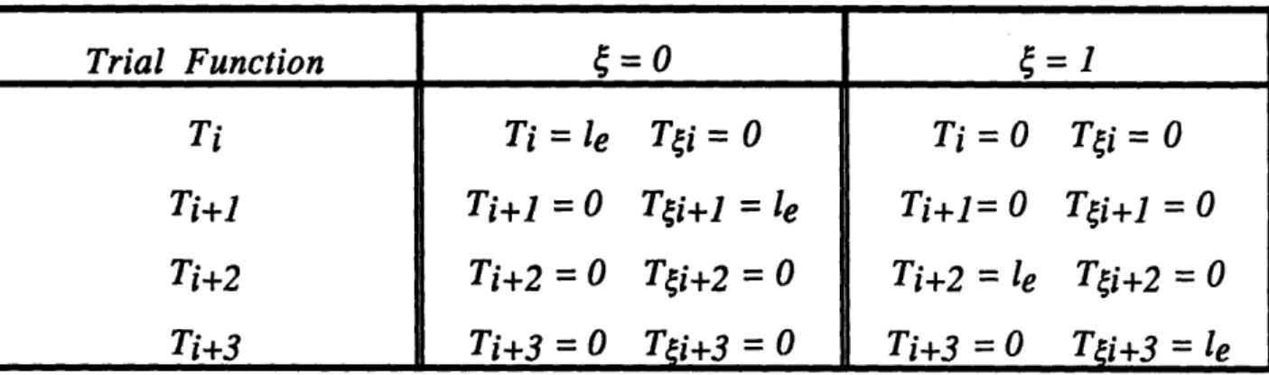
Boundary Conditions Used in Determining Cubic Trial Functions

Stiffness and Speed Parameters Used in Simulations

Numerical Value of Parameters Used for Free-Free Mode Shapes

LIST OF FIGURES

TITLE

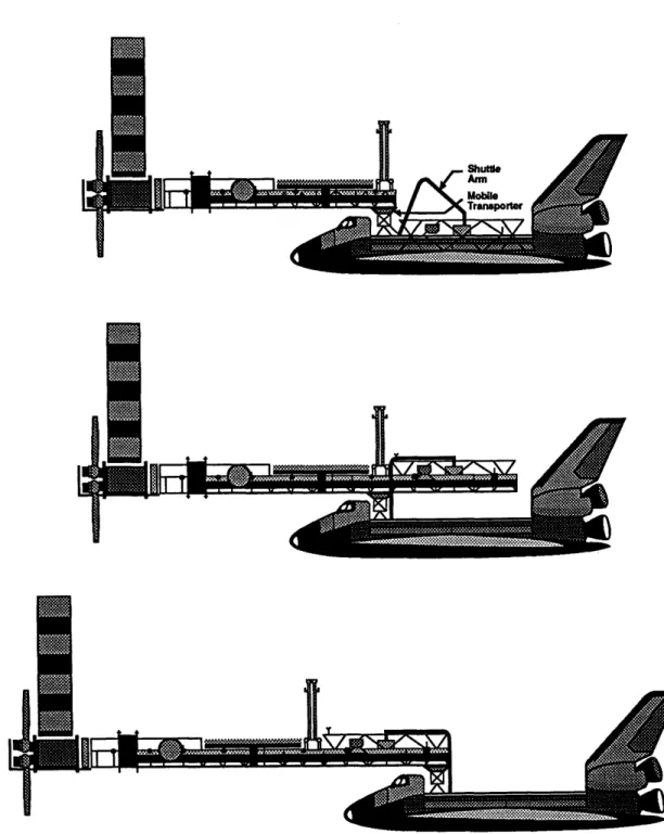
Space Station Freedom Assembly

Simply-Supported Beam With a Mass Moving Along its Length

Free-Free Beam With a Mass Moving Along its Length

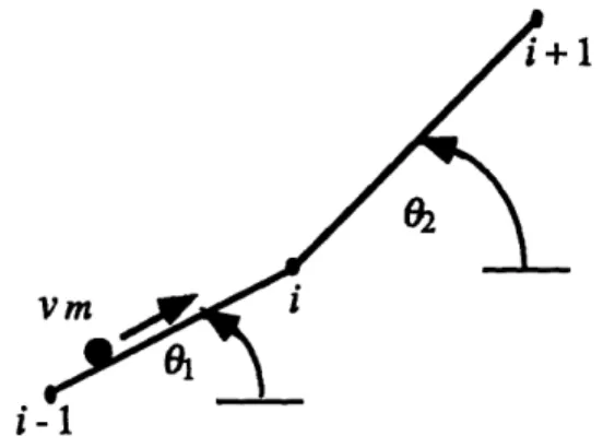
Difference in Slope of Two Neighboring Finite Elements TABLE C-1 FIGURE PAGE 56 99 180 PAGE 2 14 14 72

Mass Attached to Beam at Two Points of Contact

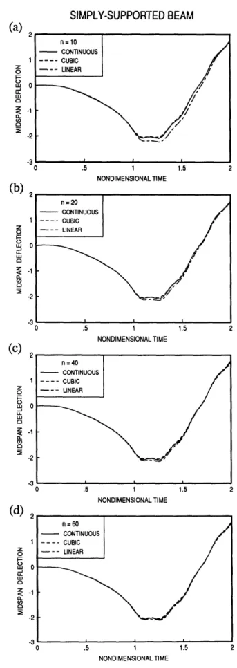
Discrete vs continuous for a = 1.0, Um = 0.5

Simply-Supported Beam

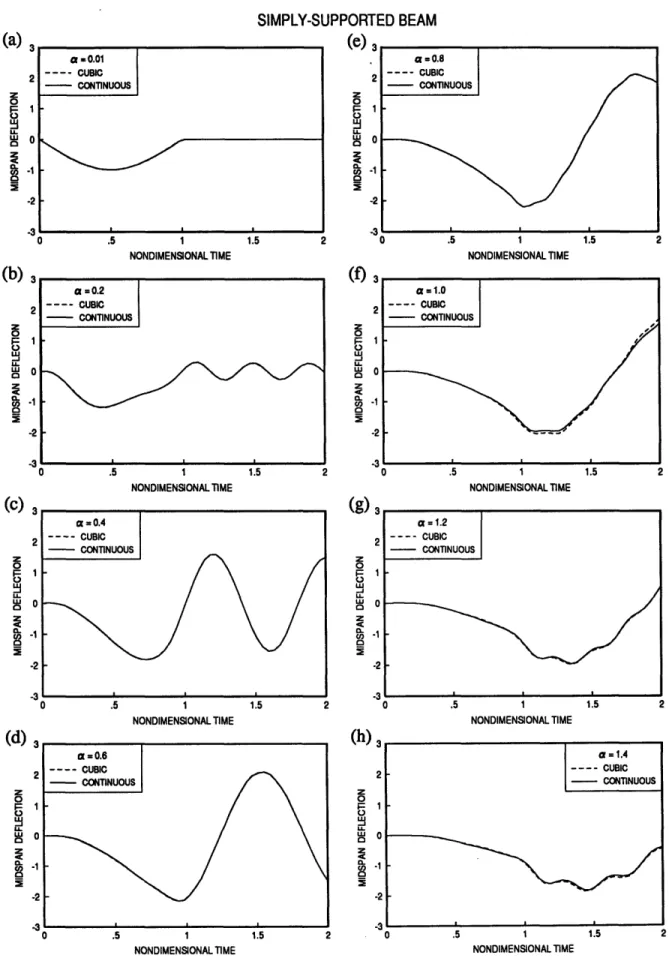
Discrete vs continuous for varying a, pm = 0.5

Simply-Supported Beam

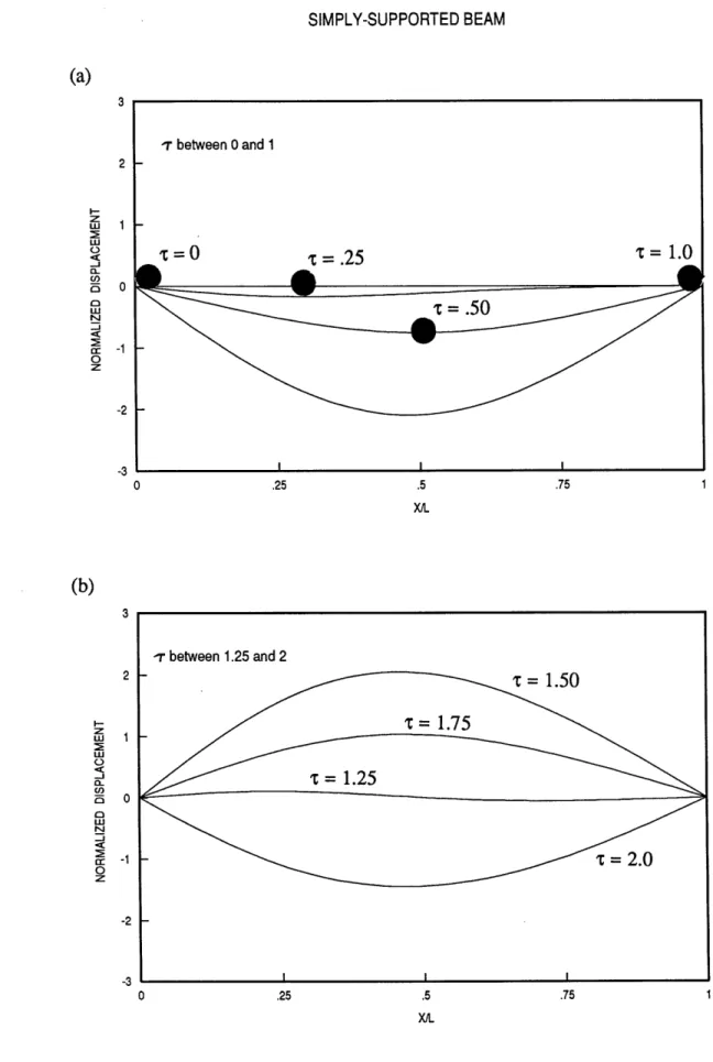
Very large values of a, Mm = 0.5 Simply-Supported Beam

Snapshot of beam with a = Simply-Supported MM vs MF for different Simply-Supported MM vs MF for different Simply-Supported 0.6 _{, lm = 0.5} Beam a, um = 0.5 Beam 113 pm, a = 0.3 Beam

Disc. vs cont. for varying a, Mm = 0.5, x = 0

Free-Free Beam

Disc. vs cont. for varying a, ym = 0.5, x = L

Free-Free Beam 78 104 106 108 110 111 10 11 12 13 115 116

14

15

Snapshot of beam with a = 0.6, #m = 0.5

Free-Free Beam

With and without moving mass for varying

a, #m = 0.5, x = 0 Free-Free Beam

With and without moving mass for varying

a, Pm = 0.5, x = L Free-Free Beam

With and without MM for varying#m, a = 0.6, x = 0 Free-Free Beam

With and without MM for varying ym, a = 0.6, x = L Free-Free Beam

Different spacing for varying a, #m = 0.5, x = 0

Free-Free Beam

Different spacing for varying a, pm = 0.5, x = L

Free-Free Beam

Model for Lagrangian Formulation

Flowchart for Numerical Simulations 16 17 18 19 20 A-1 D-1 118 119 120 122 123 125 126 149 187

CHAPTER 1 INTRODUCTION

The concept of "Freedom" Space Station divulges a wide range of dynamics problems. The particular problem considered in this thesis will help examine how the mobile transporter motion affects the space station dynamics. In the current space station layout, the mobile transporter is connected to the main truss of the space station (see Figure 1). The mobile transporter moves along the length of the truss on a track carrying payload about the station. Since the sum of the mass of the mobile transporter and that of the payload it will carry is potentially comparable to the mass of the entire station, the inertial effects of the transporter should not be ignored.

The current analysis is motivated by the Space Station-Mobile Transporter (SS-MT) system. A simplified model of a mass moving

over a flexible guideway is used to resemble the more complicated SS-MT system. This simplified system may be solved with a

continuous formulation, but obtaining a continuous formulation that will simulate the complicated system containing the station,

transporter, and shuttle is not feasible. Therefore, while a continuous analysis provides insight, a more general discrete formulation is needed to address the large-scale problem at hand.

.Shute

E

"7

W

L-Figure 1. Space Station Assembly.

!

I

The objective is to develop a discrete algorithm that can be tested against a continuous formulation for the Flexible

Structure/Moving Mass system. Once the validity of this discrete algorithm is proven, it may be extended to simulate the motion of the Space Station-Mobile Transporter system.

In both the continuous and the discrete analyses, the guideway is modeled as a flexible beam. The moving mass is considered to be a rigid body that moves along the beam's length. The inertial effects due to the motion of the mass are included in the derivation. For the discrete system, the flexible beam is divided into finite

beam-elements. Using lumped-parameter and energy-consistent methods, respectively, the beam's mass and stiffness matrices are obtained. Then, an invertible operator is used to map the continuous spatial representation of the moving mass onto the discrete representation of the flexible structure.

A continuous and discrete formulation is used to examine the mass connected to the flexible guideway at only one point. This model does not correspond to the actual Space Station-Mobile Transporter system but it serves as an appropriate test article. A continuous formulation is developed to check the results of the discrete method, and numerical results are presented for a simply-supported and a free-free flexible beam. Once the validity of the

discrete methodology is established, parametric studies are

performed for both the simply-supported and the free-free beams.

The final step in the analysis is to connect the moving mass to the flexible beam at two points. This model was chosen to represent the train/track aspect of the SS-MT system. Since a discrete

methodology was validated, a continuous formulation of this new system is not necessary. To stay close to the SS-MT system, only the free-free beam case is examined here. Studies that examine how the spacing of the two contact points affects the dynamics of the entire system are presented.

There are four chapters and four Appendices following this introduction. Chapter 2 examines the relevant work that has been

accomplished in this area. Most previous work concentrates on the motion of a truck travelling over a flexible bridge or on a train travelling over a track. The SS-MT dynamics are similar to the flexible bridge problem except for the rigid body motion that the inertially-free space station undergoes. Due to the increase in

computer power in recent years, many dynamic simulation programs were developed. Chapter 2 also examines how well these existing dynamic codes can handle the specific problem at hand.

Chapter 3 describes the theoretical analysis: Section 3.1 focuses on the continuous formulation and Section 3.2 develops the

discrete formulation. The simply-supported and the free-free beam are examined here as special cases. Section 3.3 discusses the

discrete, inertially free, multipoint-of-contact system. Each of the three sections in Chapter 3 starts with a mathematical model of the system. Then the equation of motion is developed using a Newtonian method. The equations are made nondimensional and placed into a reduced set of modal coordinates. The final equations are then cast in state-space form, which is well suited for numerical computation.

Chapter 4 displays the numerical results, and is divided into two sections. The first section, Section 4.1, outlines how the

simulations are organized, and discusses the goals that the results are trying to obtain and the parameters used to develop the simulations. The second section, Section 4.2, displays and discusses each

simulation that is run. In this section, the simply-supported case is examined first to compare the accuracy of the discrete and

continuous formulations. Parametric studies are then performed in order to examine how a change in the system nondimensional

parameters changes the system dynamics. Next, the free-free case is examined. Once again, the discrete and continuous formulations are compared to assess the accuracy of the discrete formulation.

Parametric studies are again performed when the accuracy of the discrete case has been proved. Finally the two-point-of-contact case is displayed.

Chapter 5 offers conclusions and suggestions for further work; in particular, extending the discrete formulation presented here to model the Space Station-Mobile Transporter system. The concept of connecting the shuttle to the SS-MT system could also be considered, which would be a logical extension of the work presented in this thesis.

Appendix A offers a Lagrangian formulation of the continuous free-free beam, which is used to check the continuous formulation of the same system derived earlier using Newton's equation of motion. Appendix B describes the numerical integration process that was used to obtain the simulation results shown in Chapter 4. The Runge Kutta integration scheme is described. Appendix C provides

numerical values of the matrices used in evaluating the free-free beam and expands the spatial derivatives of the shape functions used in the discrete formulations. Appendix D describes the Matlab programs that were written to simulate the Flexible

Structure/Moving Mass system. Some selected MATLAB programs are displayed.

CHAPTER 2 PREVIOUS WORKS

Reaching as far back as the early nineteenth century, scientists and theorists have been intrigued by the dynamic interaction that occurs when a load travels over a flexible structure. In the past, common models of this interactive system have been that of a truck travelling over a bridge, a train travelling along a track, or a package moving on a conveyer belt. These systems are similar to the

inertially free Flexible Structure/Moving Mass system that is used here to resemble the Space Station-Mobile Transporter (SS-MT) system.

Unlike the other systems mentioned, the Space Station-Mobile Transporter system is inertially free, and it is geometrically complex. It is necessary to obtain a discrete representation of the Flexible

Structure/Moving Mass system that can be extended to the Space Station-Mobile Transporter system. A discrete representation is necessary in order to accommodate mass and stiffness matrices, rather than partial differential equations. References [1] and [2] were the first to address this important concept in a general way. This thesis is a detailed compilation of the analysis presented in those two papers, with the exception that Ref. [2] addresses the problem of a flexible structure moving on a flexible structure.

This chapter introduces other work involving the dynamic interaction of the moving mass/flexible structure issue. Section 2.1 discusses some related previously released papers. Section 2.2 examines some existing multibody dynamics and finite-element codes in order to determine their ability to handle the proposed problem.

2.1 PREVIOUSLY PUBLISHED PAPERS

Three important features are needed to handle the Space Station-Mobile Transporter system and the dynamics of the Space Shuttle:

(1) A discrete representation.

(2) The ability to handle very large complex systems. (3) Computational efficiency.

None of the previously published papers are well suited to meet all three of these requirements. Most of the previous work assumes that a continuous model of the flexible structure is available (Refs. [3]-[7]). References [3]-[6] assume that the beam is

simply-supported. For example, Galerkin's method (Ref. [3]), Inverse Laplace transform (Ref. [5]), and Fourier series (Ref. [6]) are several of the

outlined in Section 3.2 uses the continuous solution presented in Ref. [5] for its comparison.

Reference [7] presents a continuous formulation that may be applied to different boundary conditions. This continuous solution, however, is primarily beneficial when the inertial effects of the moving mass can be ignored, thus treating the travelling load as a moving force rather than as a moving mass. The repercussions of this assumption are disclosed in Chapter 4.

Two papers (Refs. [8] and [9]) present discrete methodologies capable of solving the moving mass/flexible structure problem. Reference [8] presents a methodology that is applicable for time-varying forces. Reference [9] presents a formulation that may be implemented into a general finite-element code, such as MSC NASTRAN. This method is valid for any boundary condition. Lagrange multipliers are used to obtain a linear time-invariant

formulation, which can then be solved using NASTRAN. However, as explained in Ref. [2], this formulation is generally applicable when modal reduction is not necessary.

The papers discussed above (Refs. [3]-[9]) present

methodologies that are well suited to study the motion of a heavy truck or train travelling over a flexible bridge. However, the

free Space Station-Mobile Transporter system. It is a discrete

representation that is independent on the boundary conditions of the beam. It is well suited for model reduction so can be altered to

include the Space Shuttle's dynamics.

2.2 EXISTING CODES

In the past twenty years, the availability and power of computers has grown exponentially. Coinciding with the boom in computer hardware was an increase in computer software

capabilities. Today there are hundreds of software packages available to handle very diverse tasks.

Among the codes that handle multibody dynamic interactions are: DISCOS (Ref. [10]), ADAMS (Ref. [11]), and DADS (Ref. [12]). These codes model the connection between two bodies as either a prismatic or a rotational joint. As was stated in Ref. [1], however, the motion of the Mobile Transporter is dependent on the flexible-body motion of the Space Station. Therefore, the SS-MT system cannot be modeled using these joints, without making far-reaching

assumptions.

An alternative is to develop a formulation that could be implemented using an existing finite-element code, such as MSC NASTRAN (Ref. [13]) or ADINA (Ref. [14]). NASTRAN requires that

the equations be cast in a linear time-invariant form. Ref. [9] presents an effective approach to using NASTRAN for the moving mass problem in the case of low-order structures. ADINA's strength lies in other areas.

The discrete formulation presented in Section 3.2 is developed specifically with the application to large structural systems in mind.

CHAPTER 3

THEORETICAL ANALYSIS

Chapter 3 discusses the theoretical analysis: Section 3.1 presents the continuous formulation, Section 3.2 presents the discrete formulation with one point of contact, and Section 3.3

presents a discrete formulation for the multipoint-of-contact system.

Each section is set up in a similar manner. First, a

mathematical model of the system is discussed. Using this model, equations of motion of the entire system are developed and placed into a nondimensional form in terms of the beam's modal

coordinates. Then a state space matrix representation is formed so the formulation is suitable for numerical evaluation.

A general formulation valid for any boundary condition is presented in each section. Two systems are examined in detail: (1) the simply-supported beam and (2) the free-free beam.

3.1 CONTINUOUS FORMULATION

In the following sections, the continuous formulation of the SS-MT system is developed. The results from this formulation are compared to those obtained by the discrete analysis presented in Section 3.2.

Two different systems are examined here. The first system system model, shown in Figure 2, represents the inertially fixed space station with the transporter travelling along its length. This model represents many physical entities, the most popular example being a heavy truck travelling over a flexible bridge. The second system, shown in Figure 3, represents the inertially free space station with the transporter travelling along its length.

Vm

X

Figure 2. Simply-supported beam with a mass moving along its length.

Vm

The dynamics analysis presented is a general methodology applicable to both systems. In Sections 3.1.5 and 3.1.6, the equations are made specific to the inertially fixed and the inertially free

systems, respectively.

3.1.1 Mathematical Model

There are several ways to formulate the equations of motion for the systems depicted in Figures 2 and 3. For an inertially fixed system, an exact continuous solution using an inverse Laplace transform may be used (Ref. [5]). For a more general system, an exact continuous solution is not available.

In this analysis, however, an assumed modes approach, which accurately gives the deformation while retaining only three modes, is used to solve the systems shown in the above figures. The assumed modes approach uses Galerkin's method to determine the beam deformation due to the motion of the mass. Galerkin's method assumes that the beam deflection can be approximated by a

superposition of orthogonal mode shapes. The assumption here is that, using orthogonal modes, the error of the approximation

vanishes as the number of modes retained is increased.

The inertial effects of the moving mass are included in this analysis. If these effects are ignored, the mobile transporter is

modeled as a moving force rather than as a moving mass. If the mass of the moving object is considered negligible compared to that of the flexible structure, the inertial effects can be ignored; however, if the mass of the object is comparable in size to the structure, these inertial effects should not be ignored.

Several cases of the two approaches for different moving object/flexible structure mass ratios were studied. The results are presented in Chapter 4. In the continuous and the discrete

formulations, the flexible structure is modeled as a Bernouille-Euler beam.

3.1.2 Equations of Motion

The equations of motion for the flexible beam-moving mass system are derived in three steps:

(1) The partial differential equation describing the motion of the flexible structure is determined.

(2) The moving mass equation is obtained.

(3) A compatibility condition is invoked to obtain the equation of motion for the entire system. The compatibility

condition is a direct consequence of Newton's third law. It states that for every force there is a reactive force equal in magnitude but opposite in direction. Thus, the force on the

beam due to the moving mass is equal to the force created by the acceleration of the mass but opposite in direction.

Flexible Structure Equation

The fourth-order partial differential equation describing the motion for a Bernoulli-Euler beam is (Ref. [15]):

p ii(x,t) + EI 4 (x,t)= Fext (,t)

ax4

(3.1)

The displacement field, u(x,t), describes the motion of the mean chord of the deformed beam with respect to an inertial reference frame. This field contains any rigid body translation and rotation as well as flexible motion of the beam. Since the structure is modeled as a Bernouille-Euler beam, the mean chord of the beam is assumed to undergo pure translation as a result of the deformation. Fext is the vector sum of the external forces applied to the beam. The material properties of the beam are considered to be homogeneous.

Moving Mass Equation

The equation describing the motion of the moving mass is considered. This equation is derived using Newton's second law of mechanics, which states that the force exerted on the mass is

mm (2um (Xm (x t) t) _{= Fm (Xm (x,t),t)}

St abs _(3.2)

where Fm(xm(x,t),t) is the force exerted on the moving mass.

The absolute acceleration of the beam is the acceleration of the moving mass displacement field, um(xm(x,t),t), with respect to an inertial reference frame. When differentiating the moving mass's displacement field, it is important to imagine a reference frame embedded in the moving mass. Since the mass is moving, the

reference frame is also moving with respect to the inertial frame and adds its own terms to the acceleration of the mass. In this analysis, the mass is moving at a constant velocity vm. Therefore, the

absolute acceleration of the moving mass is

2 2 2

um am 2 am 2

() - 'm + 2 Vm++ Vm

at 2 _{t xm axm}

(3.3)

where the functional dependence of the variables are omitted for brevity.

As it stands, Eq. (3.3) is written as a function of the moving mass displacement field, um. To easily formulate the system

equation, it would be helpful to express this equation in terms of the beam's displacement u. Since the mass is fixed to the beam, it cannot

slip and, at any time, the beam and the moving mass have the same displacement in terms of Fm. This relationship can be expressed mathematically by using the dirac delta function, which is a

continuous function that depicts the value of a function at discrete times. Using this, the displacement of the mass is rewritten as a function of the displacement of the beam:

Um = Um 6(x - Xm) _(3.4)

Since the dirac delta function is not a function of time, the spatial derivatives in Eq. (3.3) are rewritten as

2 2

a

axm

ax

a um

a

u

axmat

ax at

_(3.6)

Equations (3.5) and (3.6) are substituted into the absolute

acceleration expression for the moving mass. The force equation for the moving mass then can be written in a form more compatible to the flexible beam equation:

2

2

mm

iK

-

(x-

Compatibility Equation

Newton's third law of dynamics states that for every force there is a reactive force equal in magnitude but opposite in direction. Using this law, the compatibility equation between the moving mass

and the flexible beam is determined. The force exerted on the beam due to the moving mass is equal in magnitude but opposite in

direction to the force defined by Eq. (3.7). The total force exerted on the beam is the sum of the force due to the moving mass plus any other external forces acting on the beam:

Fext = .fext - Fm (3.8)

where fext is any arbitrary external force. The external force

applied to the beam varies depending on which environment is being simulated. The actual value of fext for the two systems studied is shown in Sections 3.1.5 and 3.1.6. Using Eq. (3.7) the total force applied to the beam is

2 21

asu

Fext =fext mm ii + 2 vm + Vm (x - xm)

at ax

ax2J

_(3.9)

System Equation

The equation of motion for the entire system is obtained by using the force expression found in Eq. (3.9) and substituting it into

the beam equation (Eq. (3.1)). For clarity, any terms involving the displacement of the beam are shown on the left-hand side of the equation even though they appear due to the force exerted by the

moving mass. A fourth-order partial differential equation describing the total displacement of the beam as a mass moves at a constant velocity along its length is

a 4 U a 2 21

El + mm +i 2 vm + vm - (X - Xm) =f ext

Sx 4 _{at ax}

JX2

'I he displacement field can contain translations and rotations. The boundary condition of the beam does not change the form of this general equation.

Modal Solution

Equation 3.10 must be rewritten into a form more suitable for numerical computation. For certain systems, this equation can be solved directly using an inverse Laplace transform. A more general approach is described here. A linear superposition of orthogonal modes is used to represent the beam's vibration. The new modal representation contains a mode shape,

41,

N

where N is the number of modes. As the number of modes

approaches infinity, the modal approximation approaches the exact displacement of the beam u(x,t). The actual modes used depend on the system being analyzed. The mode shapes used for the

simply-supported and free-free beam systems are shown in Sections 3.1.5 and 3.1.6, respectively.

It is not feasible to use an infinite amount of modes to model the displacement. Different variations of the assumed modes

approach that drive the error of the approximation to zero for a small amount of modes have been developed. One of these methods is known as Galerkin's method, which uses the orthogonal property of the modes to drive the error to zero.

Equation (3.11) is used to substitute the modal coordinate l7i(t) for the natural coordinate u(x,t); this substitution is used in Eq.

(3.10). This new equation can be integrated since the mode shapes Oi are not a function of time. Before the integration takes place, the new equation is premultiplied by the transpose of the mode shapes 0j(t). Since the modes are orthogonal, this step reduces the error of the approximation. The resulting integral equation is

N

_I

o

The roman numeral superscript indicates a spatial derivative of the appropriate order. A special relationship involving the dirac delta function was used in obtaining the above equation

f

f

(x) (x

-

d =

f

(xm)

(3.14)

Nondimensional Integrals

The mode shapes are only a function of space; therefore, the integral in Eq. (3.12) can be determined either analytically or numerically. To condense the equation into a more readable form, two nondimensional integrals are defined (Eqs. (3.15), (3.16)). The values of Il and 12 for the simply-supported beam are found in Section 3.1.5. The values of the free-free beam are listed in

L

L

12

(ij)

L' *100"

o

dx

Equation (3.12) is rewritten using the definitions in Eqs. (3.15) and (3.16).

p'L II (ij) 7i

+ E1 2 ()0ri

+

i=1 L3

MMm

5

0i

i=l 1

j= 1, 2, ... N

(3.17)

Equation (3.17) represents n first-order differential equations describing the total modal displacement of the system. Next, Eq. (3.17) must be put into a nondimensional form.

Nondimensional Equations of Motion

A general procedure for placing the equations of motion into a nondimensional form is presented. First, the reference parameters for each variable in the equation must be defined. Then, each variable is divided by the appropriate reference parameter. The reference parameters for the mass, time, and length variables are:

Mass -- pL _(3.18)

Time -_ L

vm _(3.19)

Displacement - L _(3.20)

The mass terms are made nondimensional by the beam's mass. The time reference parameter is the time required for the moving mass to travel the beam's length. The beam's length is used as the

reference parameter for displacement.

For clarity, nondimensional parameters are defined below and appear after the terms are divided by their respective reference parameters.

ii

= o i tr _vm i L _(3.21)

mm #m = mm

pL

L

fl•ext t 2= f7iext

pL2

pv2m

where mt, is the reference time defined above. The parameters represent the frequency, mass, stiffness, time, and external force of the system, respectively. In the following equations, an over-script o is used to represent a derivative with respect to the

nondimensional time parameter r, i.e.,

a

tra

La

- r t t vmat (3.26)

Using the nondimensional procedure outlined previously, Eq. (3.17) is made nondimensional: (I (l

(id)

EL t2

pL

tr

(3.25)

Equation (3.27) describes the displacement of the modal coordinate due to the motion of a moving mass and an externally applied force. Next, this equation must be rewritten in a form suitable for

numerical simulation.

3.1.4 State Space Representation

The system depicted in Eq. (3.27) is described using a state-determined mathematical model. In this type of model, the system is described by a set of ordinary differential equations in terms of state variables (Ref. [16]). The future of all the variables associated with the system is predicted from the previous time history of the state variables. The only information needed about the system is the initial condition of the state variables and the equations defining the future time history of these variables.

To obtain a state space representation, an nth-order differential equation must be transformed into n first-order differential equations. Equation (3.27) is already in the required form. Next, an arbitrary set of state variables are chosen. For this model, the modal displacements and their associated velocities are chosen as the state variables: the displacements are chosen since they are the desired output, and the velocities are chosen so the

matrices take on a familiar form. The two sets of state variables are combined into one state vector

x = t_{lN..z 7N... ? 0l (3.28)}

In a state-determined formulation, the time derivative of the state vector is a function of the state variables

o

x = F(x) _(3.29)

Equations (3.28) and (3.29) show that the acceleration at any point can be expressed as a function of the velocity and displacement at that point. Once the accelerations are known, the velocities and displacements are obtained by numerically integrating the system equation of motion forward in time.

Matrix Representation

For easy evaluation, Eq. (3.27) is placed into a matrix

representation describing the states of the system. The equation is first rewritten so that it follows the standard matrix equation

describing a dynamical system

where M, C, K, and F represent the mass, damping, stiffness, and force matrices, respectively. 47 is the vector containing the modal displacements

n=[

The definition of the state vector is used to place Eq. (3.30) into the form of Eq. (3.29). The final result is an equation that can be

integrated to obtain the modal displacements and the modal velocities:

o

0

E

0

X= _X+

- M'1_{K - M'C M'}1_{F (3.32)}

where E is the identity matrix.

Additional terms representing structural damping are added to the damping matrix. It is easier to represent structural damping in modal coordinates rather than natural coordinates; therefore, the additional terms are already in modal form. Any off-diagonal modal terms are assumed to be negligible so the only extra terms appear on the diagonal. From Ref. [15], modal damping takes the form

where 2Di is the nondimensional frequency of the beam. The beam's frequency depends on its boundary condition. The natural

frequencies for the two systems examined are shown in Sections 3.1.5 and 3.1.6.

The mass, stiffness, and damping matrices all contain a constant and a time-varying component. The form of the force matrix depends on the type of external force applied to the system. The constant matrix is diagonal and represents the dynamics of the flexible beam without any moving mass. The time-varying matrix is fully populated and comes directly from the inertial effects of the moving mass. The combination of both matrices forms the total mass, stiffness, and damping matrices that are fully populated and time-varying. The constant matrices have the subscript o and the time-varying matrices have the subscript var. The total matrices are the sum of the two:

M = Mo + Mvar (3.34)

C= Co+ Cvar (3.35)

K = Ko + Kvar (3.36)

First, the constant mass and stiffness matrices are determined. The constant modal damping matrix was defined by Eq. (3.33). Even

though the actual values of the integrals have not been shown, the mode shapes used are orthogonal, ensuring the corresponding

matrices will be diagonal.

[Mo]ii

=

11(i,i)

(3.37)

[Ko]iji = 1 2(ii) _(3.38)

Next, the time-varying matrices are shown. Note that in the following matrices the mode shapes and their derivatives are

evaluated at the position of the moving mass, xm. Since xm depends on time, the values of the matrices also vary with time.

[Mvar]ijj= _{Am 1i j (3.39)}

[Cvarij = 2 /m 0i O _(3.40)

[Kvar]ij = _{m Oij l (3.41)}

As stated previously, the vector containing the external forces may or may not be time varying, depending on the actual value of the external force applied. In symbolic terms, the force vector is

F= (3.42)

The matrices shown in the Eqs. (3.37), (3.38), (3.39), (3.40), (3.41), and (3.42) are used in Eq. (3.32). The resulting expression is then numerically integrated to obtain the modal displacements and velocities at every point in time. Using Eq. (3.11) the modal

displacements are transformed into the desired natural displacements.

To reiterate, the analysis presented so far has been for the general flexible beam/moving mass system. Two systems are examined in detail using numerical methods: the inertially fixed system, which is modeled using a simply-supported beam, and inertially free system, which is modeled using a free-free beam. Both systems are explained in greater detail in Sections 3.1.5 and 3.1.6, respectively.

3.1.5 Applications to a Simply-Supported Beam

The simply-supported system shown in Figure 2 represents many different physical systems. The most common physical system associated with this model is a truck traveling over a flexible bridge. The simply-supported beam model is used in this analysis to check the discrete methodology. One advantage of using this model is the availability of previously published results. Another advantage of simulating this system is the simplicity of the mode shapes. The

nondimensional integrals can be calculated by hand; therefore, the numerical code used to simulate the system is easily checked when the simply-supported modes are used.

The modes of a simply-supported beam are (Ref. [17]) oi (x) = sini ix

L (3.43)

These modes are orthogonal but not orthonormal. The corresponding nondimensional frequencies of the beam are

vm

(3.44)

which are used in Eq. (3.33) to determine the constant component of the nondimensional damping matrix.

Once the mode shapes are known, the values of the

nondimensional frequencies are determined. For the mode shapes shown in Eq. (3.43), the integrals are determined analytically:

I (i,i) = 1

2 (3.45)

The mode shapes shown in Eq. (3.43) are also used to develop the matrices given by Eqs. (3.33)-(3.41). Since the mode shapes for this system are simple sine waves, the matrices can easily be put into their symbolic form:

Am sin rz sin N7z

-+

+/ImNsin NIz cos NIZ (3.48) 1

I

+

2

1 7 4 . 2 N 22sixSinN

x

It is easy to see the constant and time-varying components of these matrices. It is also apparent that only the total mass matrix and the constant components of the damping and stiffness matrices are symmetric. For more complex systems it is harder to write these matrices in their symbolic form.

The simply-supported beam is used to model an inertially fixed space station. To correctly model this environment, a gravitational field is imposed on the system. The external force applied to the beam is the gravitational force of the moving mass, fext = -mm g 6(x

-xm). Since the mass is moving, this force varies with time. Using Eqs. (3.13) and (3.14), the force vector used for this simulation is

EPg sin (3.50)

L g Sin NzT

j

where gXg is a nondimensional parameter for the gravitational force applied to the beam:.

mm g 2 mm g

-92tr-pL2 P V _(3.51)

The results of this simulation are presented in Chapter 4.

3.1.6 Applications to a Free-Free Beam

The free-free system, shown in Figure 3, may represent a crude model of the space station-mobile transporter system as it orbits around earth. The transporter is connected to the space

station at one point. Therefore, this model depicts the transporter as a wheel travelling over the truss, rather than as a train travelling on a track. The train/track aspect of the mobile transporter is examined in Section 3.3.

The model used to describe the inertially free system is a free-free flexible beam with the rigid transporter travelling along its length. The modes of a free-free beam are (Ref. [17])

02 =x - 1/2

Ci

= cos fi x+ cosh Pi x -oi (sin fi x + sinh fi x1

(3.52)

3 si<N

where

(3.53)

The first mode corresponds to rigid body translation. The

second mode corresponds to rigid body rotation. The next N+2 modes are the flexible modes of the free-free beam. All the mode shapes are nondimensional, orthogonal, and orthonormal. The values for Pi and ai for the first three flexible modes are located in Appendix C.

The corresponding nondimensional frequencies of the free-free beam are

I = 2 _(3.54)

which, for this system, are the frequencies used when forming the constant modal damping matrix.

For the free-free beam system, the nondimensional integrals are not determined analytically. Instead, Il and 12 are determined by numerical integration. A fourth-order Runge Kutta integration scheme (detailed in Appendix B) is used, which is the same

integration scheme used to integrate the equations of motion.

The constant matrices are formed using the nondimensional integrals and the nondimensional frequencies. The time-varying matrices are formed using the mode shapes given in Eq. (3.52) at the

appropriate value of r. There is nothing gained by writing out the specific matrices in their symbolic form for this system. The

constant mass, stiffness, and damping matrices for the first three flexible modes are available in Appendix C.

Since this system is designed to model an inertially free

system, there is no gravitational field present. An initial vibration or an external force is needed to excite the system. For this simulation, an initial vibration was used rather than an external force. When the SS-MT system is attached to the shuttle system it is possible for the first mode to be excited due to the attitude control system of the

shuttle. To create an initial excitation the left and right tip

deformations were set equal to .02L with the contributions from the first mode only. The moving mass was then released onto the beam as it was vibrating. The results are presented in Chapter 4.

3.2 DISCRETE FORMULATION

Section 3.2 develops the discrete formulation of the SS-MT system that was analyzed in Section 3.1. The results obtained from this derivation are compared to the results obtained by the

continuous formulation derived in Section 3.1. As before, two different systems are examined. The first system model, shown in Figure 2, represents a moving mass traveling along an inertially fixed structure. The second system, shown in Figure 3, represents the mass moving over an inertially free structure such as the space station.

A general methodology is presented for analyzing any system. In Sections 3.2.5 and 3.2.6 the methodology is made specific for the two systems described above.

3.2.1 Mathematical Model

In this formulation, the continuous systems of the previous sections will be placed into a discrete representation. As stated previously, a Bernouille-Euler beam is used to model the flexible

structure. Discrete mass and stiffness matrices are determined for the flexible beam. The deflection of the beam and all the external forces applied to the beam are made discrete by introducing an

invertible operator that distributes the effects of the moving mass over the appropriate discrete elements.

First, the discrete equation of motion for the flexible structure is developed by creating discrete mass and stiffness matrices using either finite-element or lumped-parameter methods. These matrices represent the physical properties of the flexible structure. The goal is to discretize the load exerted on the beam due to the moving mass

so it can be used with the already existing property matrices. To achieve this, a vector is formed that distributes the continuous forces along the beam's discrete points. A vector is created using two

different finite-element shape functions: linear and cubic, which are compared in Chapter 4. Using the equivalent forces, the discrete equation is formed. To coincide with the continuous formulation, the discrete equation is formed in terms of modal coordinates. This equation is then made nondimensional and placed into state space domain. The results for the simply-supported and the free-free beam are shown in Chapter 4.

3.1.2 Equations of Motion

The discrete matrices that represent the mass and stiffness of the beam are determined and are used to write the general matrix equation of motion for a beam. This equation is the same one shown in Eq. (3.30) but is rewritten here for convenience

M q'+Cq+Kq=F

_(3.55)

where M, C, K, and F represent the mass, damping, stiffness, and force matrices, respectively. When this equation was used in Section 3.1, the matrices used represented the physical properties of the modes used to describe the motion. In the above equation, the matrices represent the discrete properties of the different beam elements used to model the beam. Even though the two equations have the same form, they represent two different systems.

First, the discrete mass and stiffness matrices are formed. A discrete matrix for the damping is not developed in this subsection; however, a modal damping matrix is introduced in Section 3.2.4. The discrete stiffness matrix is developed using finite-element (or

energy-consistent) techniques. Two different discrete mass matrices are formed. One matrix, developed from finite-element techniques, is used when it is important to keep the rotational inertias of the beam elements. The other mass matrix, formed using a lumped parameter model, is used when only the translational degrees of freedom of the beam elements are required.

Next, a vector is developed that weights the continuous force due to the mass over the discrete beam elements. This vector is also used to discretize the deflection due to the moving mass. By

combining the discrete property matrices and the discrete forces due to the moving mass, the discrete equation of motion for the system is formed.

Mass Matrix

The mass matrix for the beam is derived using both a lumped-parameter analysis and the energy-consistent finite-element method. When the linear shape function is used, the rotational degrees of

freedom are statically condensed out of the mass and stiffness

matrices; therefore, a lumped-parameter model is easily used. When the cubic shape function is used, each element's rotational degrees of freedom are needed; therefore, the mass matrix will be developed using the finite-element method.

Lumped-Parameter Model. The lumped-parameter method is appropriate only when the beam's material properties are

homogeneous. In this particular analysis, this requirement is met; therefore, the model is valid. First, the beam is broken up into n finite elements. Then the mass of each element is distributed

between the two neighboring nodes. In the case of the

lumped-parameter model, the mass contribution at each node is half the mass of each element. The mass of each element is

where le is the length of each element and is defined as

e n(3.57)

Since the material properties are continuous throughout the beam, the total mass at each node is the sum of the contributions from the two neighboring elements. The total mass at each node is

mi = L me + L me

2 2 _{2_in}

= me (3.58)

Since the first and last nodes only feel the effects of one finite element, the mass contribution at those nodes is half the mass contribution at the inner nodes.

Each node has a corresponding translation and rotation. Since the rotational inertias of each beam element are so small, the

rotational degree of freedom can be eliminated from the stiffness matrix by using static condensation.

When the linear shape function is used to distribute the force, only the translations at each node are important. Therefore, the mass matrix should only contain the translational degrees of

row, starting with the first row, corresponding to the translational degrees. The other rows correspond to the rotational inertias of each node. Since this will not be included in the mass matrix, the

rotational inertias have not been shown. The final translational mass matrix has n+1 degrees of freedom and is in the following form

Mt = 0 mi 0 n+1

0 0

n+1 (3.59)

This matrix is constant and discrete.

Finite-Element Model. The matrix shown in Eq. (3.59) is used with the linear shape function. However, when the cubic shape function is used it is necessary to have access to both the

translational and rotational degrees of freedom. It is possible to simply add the rotational inertias of the elements into the lumped-parameter model shown above. Instead, however, an

energy-consistent mass matrix is developed. The finite-element approach is used to show another way to obtain a discrete mass matrix and is also used for the stiffness matrix. Each element of the finite-element mass matrix is (Ref. [15])

L

m! - s1 sj dx

where si is a finite-element trial function. To correctly model a beam element, Hermites cubics are chosen for the trial functions because they have a continuous spatial second derivative (Ref. [15]). A trial function is needed for the deflection and the slope at each end of the element. Therefore, four trial functions for each element are needed. The four cubics are shown below.

ie)l le) (3.61) s2=I -2x.(&+ le le)lle)l _(3.62) S

le

le

(3.63)

To determine the mass matrix for one element, the above trial functions are substituted into Eq. (3.60). This expression is then integrated to obtain the elemental mass matrix. The mass matrix is partitoned into four different matrices

m= mele [m m12]

420 Lm 21 m2 2 (3.65)

156

22

le

M 54

-13 le

-13

le

-3 le(3.68)

E156

-22

1e

Ie

Next, the elemental mass matrices are combined to form the final global mass matrix. At this point all the degrees of freedom, translational and rotational, are present. Since the inner nodes connect two consecutive elements, the elemental mass matrices overlap. Therefore, the final global mass matrix is

m= me 420n ml l m12 0 0 0 m21 ml1 + mn22 2 M12 0 0 0 . . ". 0 0 0 '. m1 1 + m22 m1 2 0 0 0 m2 1 m2 2 (3.70)(3.70)

Stiffness Matrix

The stiffness matrix is developed using finite-element techniques. When the linear shape function is used, only the translations at each node are required. Therefore, the rotational degrees of freedom are statically condensed out. The global stiffness matrix is developed the same way as the energy-consistent mass matrix. Using the finite-element method, the elemental stiffness matrix is determined by (Ref. [15])

L

(3.71)

Once again the cubics shown in Eqs. (3.61)-(3.64) are substituted into Eq. (3.71). After integration, the elemental stiffness matrix is

obtained and, like the mass matrix, is also partitoned into four different matrices:

k

=

(EI)e

[k

II

k1

2

le k2 1 k2 2 (3.72)

where (EI)e is the elemental bending stiffness. The four matrices are

k

2

61e

(3.73)

k12 = [-12 -61e k21 = -12 61e k22 = _-61e1

61e

21,2

-61e

-61e

Next, the element stiffness matrices are combined to form the global stiffness matrix. At this point all the degrees of freedom,

translational and rotational, are present. Since the inner nodes connect two consecutive elements, the stiffness matrices overlap.

Therefore, the final global stiffness matrix is

k

(EI)e

e

When the linear shape function is used, Eq. (3.77) is altered to condense out the rotational degrees of freedom. This reduced

stiffness matrix is used in conjunction with the mass matrix shown in Eq. (3.59). For the cubic shape function, the matrix, as it stands in Eq.

(3.77), is used with the similar mass matrix shown in Eq. (3.70) that contains both the translational and rotational degrees of freedom.

The global stiffness matrix of Eq. (3.76) can again be partitoned into four separate matrices, ktt, ktr, krt, and ktt. The subscripts indicate either translational or rotational degrees of freedom. The partitoned stiffness matrix is

13e krt krr (3.78)

As stated previously, the rotational degrees of freedom are eliminated when using the linear shape function. The rotational degrees of freedom are statically condensed out. This is achieved by using the static matrix equation in Eq. (3.79):

Sktt

kr

v

krt

krr

0

0

(3.79)

where v is a generic translational coordinate and 0 is a generic

rotational coordinate. Solving for 0 in terms of the translation, v, the reduced stiffness matrix becomes

Kt = ktt - ktr krTr krt (3.80)

Eq. (3.79) is a square matrix that is constant and has (n+1) degrees of freedom. When the rotational degrees are not eliminated, the

stiffness and the matching mass matrix has (2n + 2) degrees of freedom.

Beam Equation

Using the mass and stiffness matrices defined above the beam equation of motion is determined as

Mq + K q = Ft (3.81)

where M and K are generic discrete matrices representing the

appropriate mass and stiffness matrices, depending on which case is being examined. _{The nodal displacements, contained in the q vector,} represent the displacement at each node for the different elements. The nodal displacements, q, should not be confused with the modal displacements, 77, discussed in Section 3.1.2. The total discrete force vector, Ft, is a combination of any external forces applied to the beam and the inertial effects of the moving mass. This force vector is the discrete form of the vector Ft. It correctly weights the effects of the moving mass onto the nodes of the beam. It is made discrete by using the discretization vector defined below.

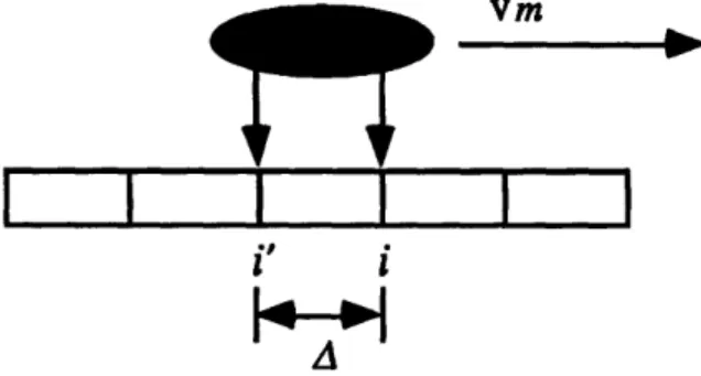
Discretization Vector

In order to weight the effects of the continuous force between two discrete nodes, an invertible operator, called the discretization vector because it places the continuous forces into a discrete form