Changes in terrestrial carbon storage during interglacials: a comparison between Eemian and Holocene

(1)

HAL Id: hal-00298137

https://hal.archives-ouvertes.fr/hal-00298137

Submitted on 17 Jul 2006

HAL is a multi-disciplinary open access archive for the deposit and dissemination of sci-entific research documents, whether they are pub-lished or not. The documents may come from teaching and research institutions in France or abroad, or from public or private research centers.

L’archive ouverte pluridisciplinaire HAL, est destinée au dépôt et à la diffusion de documents scientifiques de niveau recherche, publiés ou non, émanant des établissements d’enseignement et de recherche français ou étrangers, des laboratoires publics ou privés.

Changes in terrestrial carbon storage during

interglacials: a comparison between Eemian and

Holocene

G. Schurgers, U. Mikolajewicz, M. Gröger, E. Maier-Reimer, M. Vizcaîno, A.

Winguth

To cite this version:

G. Schurgers, U. Mikolajewicz, M. Gröger, E. Maier-Reimer, M. Vizcaîno, et al.. Changes in terrestrial carbon storage during interglacials: a comparison between Eemian and Holocene. Climate of the Past Discussions, European Geosciences Union (EGU), 2006, 2 (4), pp.449-483. �hal-00298137�

(2)

CPD

2, 449–483, 2006 Terrestrial carbon storage during interglacials G. Schurgers et al. Title Page Abstract Introduction Conclusions References Tables Figures J I J I Back Close

Full Screen / Esc

Printer-friendly Version Interactive Discussion

EGU Clim. Past Discuss., 2, 449–483, 2006

www.clim-past-discuss.net/2/449/2006/ © Author(s) 2006. This work is licensed under a Creative Commons License.

Climate of the Past Discussions

Climate of the Past Discussions is the access reviewed discussion forum of Climate of the Past

Changes in terrestrial carbon storage

during interglacials: a comparison

between Eemian and Holocene

G. Schurgers1, U. Mikolajewicz1, M. Gr ¨oger1, E. Maier-Reimer1, M. Vizca´ıno1, and A. Winguth2

1

Max Planck Institute for Meteorology, Hamburg, Germany

2

Center for Climatic Research, Department of Atmospheric and Oceanic Sciences, University of Wisconsin, USA

Received: 29 June 2006 – Accepted: 7 July 2006 – Published: 17 July 2006 Correspondence to: G. Schurgers (guy.schurgers@zmaw.de)

(3)

CPD

Full Screen / Esc

EGU Abstract

A complex earth system model (atmosphere and ocean general circulation models, ocean biogeochemistry and terrestrial biosphere) was used to perform transient simu-lations of two interglacial sections (Eemian, 128–113 ky B.P., and Holocene, 9 ky B.P.– present). The changes in terrestrial carbon storage during these interglacials were 5

studied with respect to changes in the earth’s orbit. The effect of different climate fac-tors for the changes in carbon storage were studied in offline experiments in which the vegetation model was forced with only temperature, hydrological parameters, radi-ation, or CO₂concentration from the transient runs. Although temperature caused the largest anomalies in terrestrial carbon storage, the increase in storage due to forest ex-10

pansion and increased photosynthesis in the high latitudes was nearly balanced by the decrease due to increased respiration. Large positive effects on carbon storage came from an enhanced monsoon circulation in the subtropics between 128 and 121 ky B.P. and between 9 and 6 ky B.P., and from increases in incoming radiation during summer for 45◦to 70◦N compared to a control run with present-day insolation.

15

Compared to this control run, the net effect of these changes was a positive car-bon storage anomaly of about 200 Pg C for 125 ky B.P. and 7 ky B.P., and a negative anomaly around 150 Pg C for 116 ky B.P. Although the net increases for Eemian and Holocene were rather similar, the causes of this differ substantially. The decrease in terrestrial carbon storage during the experiments was the main driver of an increase in 20

atmospheric CO₂concentration for both the Eemian and the Holocene.

1 Introduction

The historical CO₂ concentration in the atmosphere, as was derived from ice cores (Inderm ¨uhle et al.,1999), shows a rising trend for the last 8000 years, from around 260 ppm at 8 ky B.P. to around 280 ppm for the pre-industrial era. Several different 25

(4)

CPD

Full Screen / Esc

EGU storage on land (Inderm ¨uhle et al.,1999) and in the ocean (Broecker and Clark,2003),

as well as changes by mankind due to land use change (Ruddiman,2003).

A few transient simulations were performed for the Holocene to reconstruct the course of atmospheric CO₂.Brovkin et al.(2002) performed simulations with the earth system model of intermediate complexity CLIMBER, andJoos et al.(2004) performed 5

simulations with the dynamic global vegetation model LPJ coupled to an impulse-response function model for the ocean carbon cycle based on the HILDA ocean model. BothBrovkin et al.(2002) andJoos et al.(2004) obtain a reasonable reconstruction of the atmospheric CO₂concentration, covering the increase over the last 8000 years. However, the causes for the increase in the atmospheric CO₂ concentration differed 10

between these studies. In the study of Brovkin et al.(2002) the increase of the CO₂ concentration is driven by a decrease of terrestrial carbon storage of 90 Pg C over the last 8000 years, while in the study by Joos et al. (2004) it is driven by a decrease of oceanic carbon due to compensation of terrestrial uptake by sediments and ocean surface heating. In the last study, the terrestrial biosphere shows no clear uptake or 15

release of carbon for the last 8000 years. A reconstruction of terrestrial carbon storage for the Holocene byKaplan et al.(2002) had similar results as the study byJoos et al. (2004), the terrestrial carbon storage increased clearly during the early Holocene, from 8 ky B.P. a slight increase was simulated.

Reconstructions of the global vegetation distribution for the Holocene were provided 20

by the BIOME 6000 project (Prentice and Webb III, 1998; Prentice et al., 2000) for 6 ky B.P., based on pollen data, and byAdams and Faure(1997). Consistent features of mid-Holocene vegetation distribution in these and other studies are a northward expansion of the boreal forest zone in the northern hemisphere and an increase of vegetation in monsoon areas in the subtropics of the northern hemisphere.

25

In the study presented here, a complex earth system model was applied to recon-struct the carbon cycle for the Eemian and the Holocene. Carbon storage in the ter-restrial biosphere and its contribution to the atmospheric CO₂concentration were anal-ysed. The changes in terrestrial carbon storage were traced back to certain climatic

(5)

CPD

Full Screen / Esc

Printer-friendly Version Interactive Discussion EGU factors. 2 Method 2.1 Model

A complex earth system model, consisting of general circulation models for atmosphere and ocean, an ocean biogeochemistry model, and a dynamic vegetation model, was 5

used to study two interglacial sections transiently. The general circulation models for atmosphere and ocean, ECHAM3-LSG, were used in a coupled mode before for long-term experiments, both regarding paleoclimate (Mikolajewicz et al.,2003) and regard-ing anthropogenic warmregard-ing (Voss and Mikolajewicz,2001). The carbon cycle within the earth system model was represented with the dynamic global vegetation model LPJ 10

(Sitch et al.,2003) and a marine biogeochemistry model based on HAMOCC3 ( Maier-Reimer,1993), described inWinguth et al.(2005) and Mikolajewicz et al. (2006)1. The dynamic global vegetation model calculates the occurrence of ten plant functional types (PFTs), and within these PFTs, carbon is allocated between four biomass pools. Each PFT contains three litter pools, and each gridcell (which can contain more than one 15

PFT) contains two soil carbon pools. The ocean biogeochemistry model simulates the distribution of the main components for the carbon cycle, including CO₂, particulate organic carbon and CaCO₃. A sediment module was inserted to account for long-term storage or dissolution of sediments. CO₂is treated prognostically in the earth system model, changes in carbon storage on land and in the ocean influence the atmospheric 20

CO₂concentration, which is modelled as a well-mixed box.

The land surface conditions for the atmosphere were adapted according to changes 1

Mikolajewicz, U., Gr ¨oger, M., Maier-Reimer, E., Schurgers, G., Vizca´ıno, M., and Winguth, A.: Long-term effects of anthropogenic CO2emissions simulated with a complex earth system

(6)

CPD

Full Screen / Esc

EGU in the vegetation Schurgers et al. (2006).2

A version of the earth system model in which the ice sheets were treated interactively was described inWinguth et al.(2005) and Mikolajewicz et al. (2006)1, however, for this study the ice sheets were fixed at present-day conditions.

In order to enable long paleoclimate experiments with this complex model, the 5

resolution of the components is relatively low: the atmosphere and the vegetation model run on a T21 grid (roughly 5.6◦×5.6◦), the ocean and ocean biogeochemistry run on a Arakawa E-grid (effectively 4.0◦×4.0◦). A modified version of the periodically-synchronous coupling technique bySausen and Voss(1996) was applied, using fluxes at the surface rather than an energy balance model. It was described in detail in Miko-10

lajewicz et al. (2006)1. Both experiments were started from a pre-industrial control run, followed by a 1000 year spinup with insolation according to 129–128 ky B.P. (Eemian) and 10–9 ky B.P. (Holocene).

2.2 Biome descriptions

As a tool for evaluation of the vegetation distribution, a scheme was developed to 15

represent the regular output of the vegetation model in so-called biomes or macro-ecosystems. In order to compare the modelled distribution of plant functional types with vegetation reconstructions for the past, the combinations of plant functional types as were simulated by LPJ are converted into seven biome classes. Several schemes have been described in literature, the classes that are proposed here are (1) able to 20

present the major conversions that take place on longer time scales, (2) are structured in a way that is understandable and (3) can be derived from the LPJ output, without putting in too much uncertainty, but with enough distinction between them to show shifts of vegetation over long time scales. The scheme that is used here uses the fractions of coverage from the ten plant functional types from the output of the vegetation model, 25

2

Schurgers, G., Mikolajewicz, U., Gr ¨oger, M., Maier-Reimer, E., Vizca´ıno, M., and Winguth, A.: The effect of land surface changes on Eemian climate, Clim. Dynam., submitted, 2006.

(7)

CPD

Full Screen / Esc

EGU together with the soil temperature from the atmosphere model. The distribution is

explained in Table1.

2.3 Experiments

Long integrations were performed with the earth system model for the Eemian (128 ky B.P.–113 ky B.P.) and the Holocene (9 ky B.P.–present) with the complex earth 5

system model, for which insolation changes were prescribed according to Berger (1978). A control run of 10 000 years was performed with present-day insolation. CO₂ was treated prognostically in the earth system model, changes in carbon storage on land and in the ocean influence the atmospheric CO₂concentration. Ice sheets were fixed at their present-day state. Both experiments were started from a pre-industrial 10

control run followed by a 1000 year spinup with insolation according to 129–128 ky B.P. (Eemian) and 10–9 ky B.P. (Holocene).

Besides these two coupled integrations, the climate data of these experiments were used to perform experiments with the offline vegetation model. Experiments were per-formed based on control run climate, with temperatures, radiation, hydrological param-15

eters or pCO₂ from the Eemian or Holocene experiments, to determine which param-eters influence the distribution and carbon storage of vegetation most. An overview of the experiments is given in Table2.

3 Results

A general overview of climate change in the experiments will be given. It will be dis-20

cussed how changes in the climate affect variations in the carbon storage. The shifts in the distribution of vegetation will be discussed using the classification described above, and will be compared to observations and reconstructions. The influence of these shifts and of changed climate on terrestrial carbon storage will be discussed.

(8)

CPD

Full Screen / Esc

EGU 3.1 Climate change

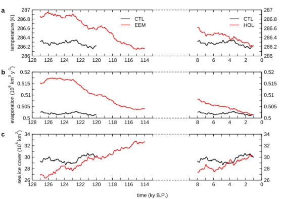
Due to changes in the incoming solar radiation, climate changes both in its annual cycle, and in its yearly mean state. For the beginning of both the Eemian and the Holocene experiment, global temperatures were higher than the control experiment by 0.5 K for 128 ky B.P. and 0.2 K for 9 ky B.P. (Fig.1a). During the two interglacials, global 5

temperature decreased towards the pre-industrial control run average. For the Eemian from 117 ky B.P. onwards, global temperature was lower than for the control run. The increased temperatures are accompanied by increased evaporation, with a maximum of 0.015×106km3y−1for the Eemian and 0.006×106km3y−1for the Holocene over the control run value (Fig.1b). Global sea ice cover shows a course consistent with the 10

global temperature: for the beginning of the insolation experiments sea ice cover is lower than for the control run by 2 to 3×106km2, and ice cover increases during the experiments (Fig.1c).

3.2 Vegetation distribution 3.2.1 Simulated changes 15

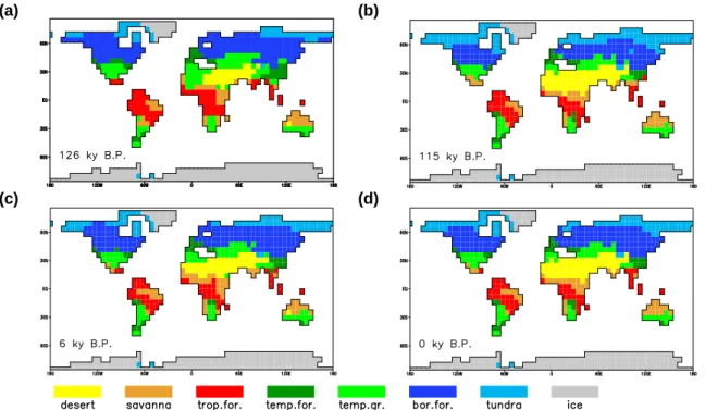
The distribution of vegetation for selected time slices in these periods is shown in Fig.2, using the biome description presented in Sect. 2.2. For present-day (Fig. 2d), the pattern matches quite well with what is considered as “potential” vegetation for most parts of the world. Remarkable deviations were simulated for the Amazon region, which is dominated by savanna in the simulation, Europe, which is too much dominated 20

by boreal forest rather than temperate forest, and Australia, which lacks large desert areas. These deviations were caused by the control run climate: the high latitudes are in general too cold, and the Amazon region is too dry.

For 6 ky B.P. (Fig. 2c), both at the northern and the southern boundary of the Sa-hara desert, as well as of the South Asian deserts, vegetation expands compared to 25

(9)

CPD

Full Screen / Esc

EGU America, and to a lesser extent the high latitudes of east Asia, boreal forest expands

compared to the control run. For 126 ky B.P. (Fig.2a), these effects are even larger. The western part of the Sahara is covered with temperate grassland in the simulation, tropical forests in northern Africa and southeast Asia expand, and the boreal forests expand northward up to the Arctic Ocean in many places. In the southern hemisphere 5

a slight retreat of forests was simulated for Africa. For 115 ky B.P. (Fig.2b), the oppo-site can be seen: boreal forests in the northern hemisphere show a clear southward retreat and the vegetation cover in the monsoon areas decreases slightly, in most other regions vegetation patterns are very similar to simulated present-day conditions.

3.2.2 Comparison with vegetation data 10

Global data sets of vegetation for paleoclimatic times are rare and provided only for selected time slices. The Holocene has been studied more often than the Eemian, which is related with the obtainability of pollen data.

For the last interglacial optimum, a reconstruction of northern hemisphere vegetation was provided byGrichuk (1992). For the high latitudes it shows a decreased tundra 15

area, coniferous forests expand northward up to the Arctic Ocean. Some tundra areas remain in northeast Asia and the northeastern part of North America. This is consistent with the simulated distribution of tundra from the Eemian experiment (Fig. 2a). The forest zone shifts northward, especially for North America. In the simulation, the border between temperate and boreal forest is too far south compared to the reconstruction. 20

The subtropical trees and bushes occupy a larger area: large parts of northern Africa are covered with savanna-type vegetation. This was found in the Eemian experiment as well, although the simulated area is restricted to the western part of Africa (Fig.2a). A large set of pollen data for central Asia during the Eemian was provided byTarasov et al. (2005), revealing an increase of taiga till 125 ky B.P., followed by a period with 25

relatively high taiga cover. At the end of the interglacial, steppe and tundra become more dominant again.

(10)

CPD

Full Screen / Esc

EGU provided byPrentice et al. (2000) for 6 ky B.P., and global vegetation maps based on

fossils, pollen data and other sources for 8 and 5 ky B.P. are provided byAdams and Faure (1997). Detailed comparison studies between data sets and model output were performed for the Mid-Holocene (6 ky B.P.) on a global scale (Harrison and Prentice, 2003) as well as in more detail for 55◦–90◦N (Kaplan et al., 2003). For 6000 year 5

B.P.,Hoelzmann et al.(1998) provided reconstructions for northern Africa as boundary conditions for modelling experiments, indicating that roughly the northern half of north Africa was mainly covered with steppe, and the southern half was mainly covered with savanna. The main features of vegetation changes in these studies were obtained in the simulation as well: a gradual southward retreat of the taiga-tundra boundary in the 10

high latitudes of the northern hemisphere, as well as a southward retreat of the border between boreal and temperate forest, and a decrease of vegetation in monsoon areas.

3.3 Terrestrial carbon storage

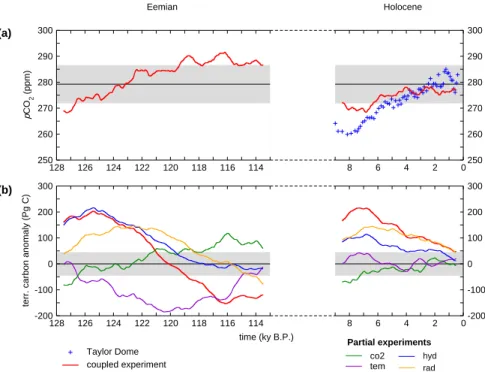
The atmospheric CO₂ concentration increased during both the Eemian and the Holocene experiment (Fig. 3a), starting around 270 ppm. For the Eemian experi-15

ment, a CO₂concentration of 280 ppm (which corresponds to the pre-industrial level) is reached around 123 ky B.P., for the Holocene experiment, pre-industrial concentration is reached at the end (0 ky B.P.). The interannual variability is remarkably large for the CTL experiment, the standard deviation is 3.6 ppm.

For both interglacials, CO₂concentration and terrestrial carbon storage show an op-20

posite tendency, with the increase of the atmospheric CO₂concentration about 40 Pg C for the Eemian and 20 Pg C for the Holocene, and the decrease of terrestrial carbon storage about 350 Pg C for the Eemian and 200 Pg C for the Holocene (Fig.3). The increase in CO₂ concentration is the result of release of terrestrial carbon (Fig. 3b), the remaining carbon released from the terrestrial biosphere is taken up by the ocean. 25

The decrease of terrestrial carbon storage was simulated for both the Eemian and the Holocene with trends of –37 Pg C yr−1(Eemian) and –31 Pg C yr−1(Holocene), and with rather similar maxima (around 205 Pg C and 215 Pg C for 125 ky B.P. and 7 ky B.P.,

(11)

CPD

Full Screen / Esc

EGU compared to the control run). After 120 ky B.P., the terrestrial carbon storage is smaller

than in the control run, with a minimum of –150 Pg C for 116 ky B.P.

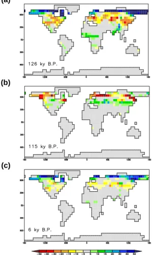
The spatial pattern for carbon storage shows that particular regions play a domi-nant role in the changes during the interglacials (Fig.4): The high latitudes north of 60◦N show an increase for 126 ky B.P. and 6 ky B.P. compared to the control run, for 5

115 ky B.P. this latitude band shows a decrease. The mid-latitudes, between 30◦N and 60◦N, show the opposite signal: a decrease of carbon storage for 126 ky B.P. and 6 ky B.P., and an increase for 115 ky B.P. The monsoon regions in northern Africa and southeast Asia show a clear increase for 126 ky B.P., and a small effect for 6 ky B.P. as well. The southern hemisphere shows some small changes, but no clear pattern can 10

be observed here.

Carbon storage anomalies for the Eemian and the Holocene can not be explained from a single climate parameter (Fig.3). All parameters analysed here (temperature, radiation, hydrology and CO₂) show effects on the total carbon storage that are larger than two standard deviations of the control run storage. These parameters were anal-15

ysed in detail, and are discussed below.

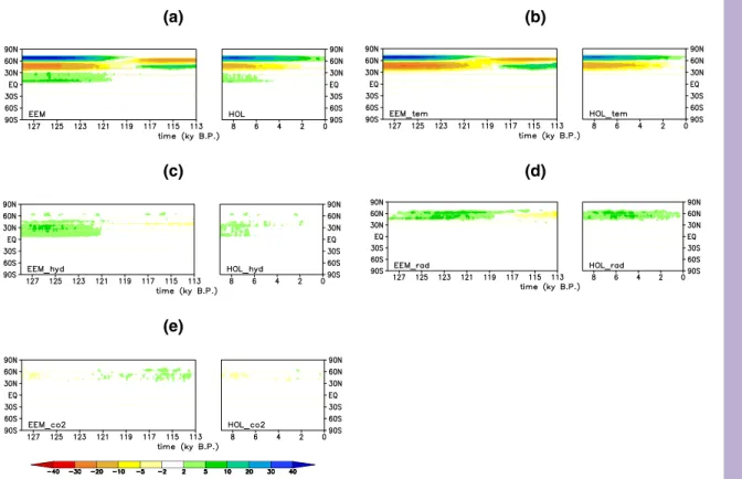
The evolution of terrestrial carbon storage in time (Fig.5a) shows the main features from the selected period in Fig.4. The bands of increased and decreased storage in the high latitudes show a remarkable swap around 120 ky B.P. From 128 to 120 ky B.P., an increase was simulated for 60◦–75◦N, a decrease for 40◦–60◦N, and again an increase 20

for 0◦–30◦N. After 120 ky B.P. the pattern shifts: a decrease was simulated for 55◦– 65◦N, and an increase is seen for 45◦–55◦N.

3.3.1 Temperature

Temperature changes during the interglacials (Fig.6) are a direct effect of changes in the earth’s orbit. Due to a summer perihelion at 127 ky B.P., combined with a large ec-25

centricity of the earth orbit, summer insolation for the northern hemisphere is enhanced compared to present-day for the first half of the Eemian experiment. This causes pos-itive temperature anomalies in summer (Fig. 6). For the second half of the Eemian

(12)

CPD

Full Screen / Esc

EGU experiment, the perihelion occurs in winter for 116 ky B.P., causing a relatively low

in-coming radiation in summer, and an increase in insolation in winter (Fig.6). For the Holocene, the effect is slightly less: although perihelion occurs in summer as well, the eccentricity is roughly half of the Eemian eccentricity, thereby reducing the differences between summer and winter (Berger,1978).

5

For the beginning of both Eemian and Holocene, the Northern Hemisphere sum-mer is warsum-mer, with a larger anomaly for the Eemian than for the Holocene. For the Eemian, warming occurs as well around the equator, the monsoon areas in the North-ern Hemisphere are relatively cool due to increased evaporation and increased cloud cover, related to an enhancement of the monsoon precipitation. For the Eemian, a 10

cooling up to 4 K occurs after 120 ky B.P. for the Northern Hemisphere north of 20◦N. A slight cooling (up to 1.5 K) was simulated for the last 2000 years of the Holocene as well, which is remarkable, and which shows that a steady-state control run does not necessarily provide the state that would be reached at the end of a transient run. For the Northern Hemisphere winter, the latitudes north of 60◦N show a clear positive 15

temperature anomaly for the beginning of both experiments. This positive anomaly changes to a negative anomaly after 120 ky B.P. A similar pattern can be seen for the Holocene, although the magnitude is slightly smaller. Again a cooling was simulated for the last 2000 years of the Holocene. The tropics and subtropics show a clear warming for winters between 122 and 114 ky B.P. In the Southern Ocean, variability is high, and 20

positive and negative temperature anomalies for summer and winter are mainly related to changes in the convection.

Temperature-induced changes in terrestrial carbon storage show the most prominent signal of all climate parameters for the mid- and high latitudes in the partial experiments (Fig. 5). For the beginning of the Eemian and Holocene experiments, an increased 25

storage of carbon is simulated in the latitudes north of 60◦N compared to the present-day situation, and a decreased storage is simulated between 40◦N and 60◦N. The anomalies become smaller with time, and for the Eemian the decrease in the high latitudes and the increase in the mid latitudes continues after 119 ky B.P., resulting in

(13)

CPD

Full Screen / Esc

EGU opposite anomalies: the high latitudes have a decreased storage and the mid-latitudes

an increased storage compared to present-day. Despite the large anomalies, the net effect on carbon storage is rather small and even negative for the Eemian experiment (Fig.3b).

For the area north of 60◦N, temperature increase causes the region to become more 5

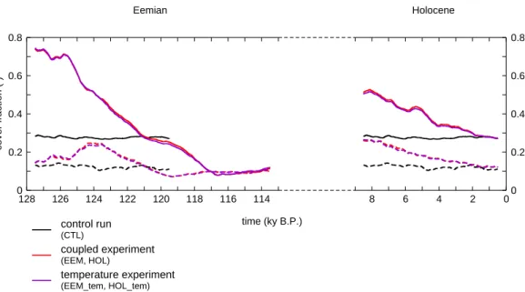
favourable for forest growth, grasses are there replaced by trees. Between 128 and 121 ky B.P., the boreal forests cover a larger area than in the control run (Fig.7). In the beginning of the experiment, the cover is over 70% of the surface. After 125 ky B.P., it declines sharply, thereby enabling a slight increase of grass cover. A decline for both boreal trees and grasses causes the covers to become lower than the control run 10

around 121 ky B.P., with a minimum forest cover of about 10% (around 117 ky B.P.). For the Holocene, a decrease of forest fraction is simulated as well, although the maximum is not as high as for the Eemian. The increase in grass cover after retreat of the forests is not seen for the Holocene, and the covers of both trees and grasses are roughly equal to the control run values at the end of the Holocene experiment.

15

In the experiments forced with temperature of the coupled experiments only (EEM tem and HOL tem) the covers of boreal forests and grasses have a very similar behaviour for the area north of 60◦N (Fig. 7), indicating that temperature is the main driver for the changes in cover fractions. These changes cause the carbon storage effect north of 60◦N. The area between 30◦N and 60◦N does not show large changes 20

in the cover fraction. The changes in carbon storage here compared to the control run are related to changes in autotrophic and heterotrophic respiration. Due to higher temperatures, decay of carbon goes faster, which causes a reduction of the residence time of carbon. Especially soil carbon pools become smaller due to the faster turnover.

3.3.2 Hydrology 25

The climate change caused by variations in the orbital forcing include changes in the hydrological cycle. Due to increased temperatures on land a stronger temperature gra-dient between the land surface and the ocean occurs and monsoon cells are

(14)

strength-CPD

Full Screen / Esc

EGU ened, thereby bringing more moist air to the continents and causing more convection.

This results in an increase of precipitation over land and a decrease over the ocean, especially in the tropics and subtropics (Fig.8a). The precipitation increase over land is substantially amplified by the positive feedback between albedo and precipitation (e.g. Claussen,1997;Braconnot et al.,1999), as was discussed in Schurgers et al. (2006)2 5

for the Eemian experiment.

Most important changes in carbon storage due to changes in the hydrological cycle take place between 10◦N and 40◦N (Fig. 5c), where water availability is a limiting factor for plant growth. Although local changes in carbon storage are smaller than the changes caused by temperature in the higher latitudes, the latitude band being 10

influenced is rather large, and the changes in the hydrological cycle cause a spatially constant positive effect on carbon storage between 128 and 121 ky B.P. and between 9 and 6 ky B.P. In contrast to temperature, there are no regional decreases in carbon storage due to hydrological changes for these periods, making hydrology one of the most important net effects of the anomalies seen for these periods in total carbon 15

storage (Fig.3b).

Figure 8a shows the positive anomaly of precipitation over the continents and the negative anomaly over the ocean between 128 and 121 ky B.P. and between 9 and 6 ky B.P. In northwest Africa, precipitation increased up to 500 mm per year compared to the pre-industrial control run. A strong increase of precipitation occurred as well 20

in the southeast Asian monsoon area around India, and at the west coast of North America. The most pronounced decrease of precipitation is found over the Atlantic Ocean, and to a lesser extend over the tropical Pacific. After 118 ky B.P., the north African as well as the North American subtropical and tropical parts of the continent become dryer than the control run.

25

Vegetation growth reacted strongly to the changes in precipitation for most regions. The most sensitive regions are northwest Africa, southeast Asia around India, and western North America, with in general strong positive anomalies in vegetation cover between 128 and 121 ky B.P. and 9 and 6 ky B.P., and smaller negative anomalies from

(15)

CPD

Full Screen / Esc

EGU 118 ky B.P. onwards (Fig. 8b). Especially for Northwest Africa and Southeast Asia,

vegetation cover was higher than present-day at the beginning of both experiments. The Eemian shows a gradual decrease of the vegetation cover in the western Sahara region from about 40% to practically 0% from 124 ky B.P. to 118 ky B.P. (Schurgers et al., 20062) . For the Holocene, maximum vegetation cover is roughly half of the Eemian 5

cover, with a decrease from 9 ky B.P. to 4 ky B.P.

The increase in vegetation cover, as well as the conversion of grass-covered areas into forests, causes an increase in carbon storage for these regions (Fig.8c). The pat-terns of carbon storage are very similar to those shown for vegetation cover, with again stronger anomalies for the Eemian than for the Holocene simulation. The maximum 10

increase in global carbon storage due to hydrological changes (from the EEM hyd and HOL hyd experiments) was roughly twice as large for the Eemian than for the Holocene (Fig.3b). This difference is directly related to the strength of the monsoon, which is mainly determined by the contrast in heating between the ocean and the land surface. Due to a decrease of the surface albedo, this contrast is enhanced. This enhancement 15

is larger for the Eemian than for the Holocene, because of the more eccentric earth or-bit for the Eemian. Besides that, the positive feedback between presence of vegetation and precipitation (see Schurgers et al., 20062, for a more detailed analysis) enhances this contrast.

3.3.3 Radiation 20

Incoming solar radiation had both for the Eemian and for the Holocene a remarkably positive direct influence on carbon storage for the latitudes between 45◦N and 70◦N during the warm phase (Fig.5). The reason for this increase is an increase in photo-synthesis for these latitudes, caused by an increase in absorbed shortwave radiation. The radiation anomaly for these latitudes (Fig.9) shows an increase of incoming ra-25

diation for the summer months and the largest decrease for spring at the beginning of the experiment. Both the positive and the negative anomaly are moving to earlier occurrence in the year, which causes the amplitude in the annual cycle of incoming

(16)

CPD

Full Screen / Esc

EGU radiation to become smaller, and both anomalies weaken during the experiments. The

incoming radiation at the surface shows a similar pattern as the incoming radiation at the top of the atmosphere, but with a smaller amplitude (not shown). Maximum in-crease in incoming radiation at the surface is around 40 W m−2 for summer around 127 ky B.P., maximum decrease is around –30 W m−2for spring 127 ky B.P. In general, 5

the amplitude at the surface is roughly 30 to 50% of the amplitude at the top of the atmosphere.

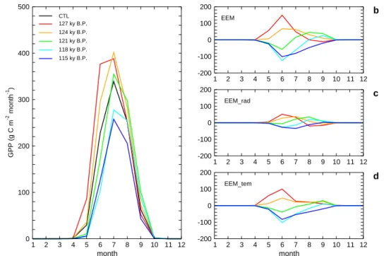
The influence of changes in the radiation on photosynthesis is shown in Fig. 10a. From 127 ky B.P. onwards, the maximum rate of photosynthesis decreased, and the peak in photosynthesis shifted later in summer. The anomalies of gross primary pro-10

duction (GPP) compared to the control run (Fig.10b) are a result of radiation and tem-perature changes (Fig.10c and d). The positive temperature anomaly both in summer and in winter for the beginning of the Eemian experiment (Fig.6) causes the growth and development of the vegetation to start earlier in the season, resulting in an increase of radiation absorption due to a faster leaf development and thereby in an increase of pho-15

tosynthesis, especially in the first two months of the growing season (Fig.10d). This effect is enhanced by a positive radiation anomaly for the summer months (Fig. 9), which results in additional photosynthesis (Fig.10c). After 122 ky B.P. the temperature anomaly became negative for the region north of 60◦N, and the development of veg-etation in spring becomes slower than in the control run. Due to the high radiation 20

anomaly, the EEM rad experiment had initially a slightly positive anomaly in GPP later in the season for 121 ky B.P. (Fig.10c), but this vanished afterwards, when the radiation anomaly decreased.

3.3.4 CO₂

Total terrestrial carbon storage in the experiments with CO₂ as varying forcing show 25

most clearly a first-order reaction to the atmospheric CO₂ concentration (Fig. 3). In these experiments, the amplitude of global net primary production (NPP) is roughly 4.5 Pg C y−1(EEM co2) and 2 Pg C y−1(HOL co2), compared to a standard deviation of

(17)

CPD

Full Screen / Esc

EGU 1.7 Pg C y−1 for the control run (CTL). These changes are small compared to changes

from other factors, and work in the opposite direction of the CO₂signal of the coupled experiments (Fig.11).

The effect of changes in the atmospheric CO₂ concentration are small on primary production and small on carbon storage, which was to be expected because the ter-5

restrial biosphere was the driver of these atmospheric CO₂changes. A terrestrial bio-sphere very sensitive to these changes would inevitably have led to a much smaller signal in the atmospheric CO₂concentration.

4 Conclusions and discussion

An earth system model was used to study terrestrial carbon storage during two inter-10

glacials, the Holocene and the Eemian. Under pre-industrial conditions, the model gives a reasonable distribution of the major vegetation zones, with some remarkable exceptions. In the Amazon region, large areas are covered with savanna type vegeta-tion, because the simulated climate is too dry here. The border between temperate and boreal forests was situated too far south, due to too cold temperatures in the Northern 15

Hemisphere mid and high latitudes.

For the beginning of the Eemian and Holocene simulations, enhanced vegetation growth in north Africa and Asia around India caused a decrease of the desert area and an increase in savanna and temperate grassland. This is in agreement with proxy data and reconstructions (e.g.Prentice et al.,2000). The cover of forests in the high lati-20

tudes of the northern hemisphere decreased during both experiments due to a gradual cooling. This causes a southward retreat of the treeline, which agrees with reconstruc-tions (Adams and Faure,1997;Prentice et al.,2000).

The changes in the distribution of vegetation, together with changes in photosyn-thesis rates, and changes in climatic circumstances, cause changes in the storage of 25

carbon in the terrestrial biosphere. These were the main cause for a gradual increase of the atmospheric CO₂ concentration during both interglacial experiments. For both

(18)

CPD

Full Screen / Esc

EGU the Eemian and the Holocene, terrestrial carbon storage was high in the beginning

of the experiments, and gradually decreased from 125 ky B.P. and 8 ky B.P. onwards. These changes can be explained by the following relations between climate and the terrestrial carbon cycle.

Temperature affected carbon storage dominantly, but its global net effect is small: 5

the increase in summer temperature of the mid and high latitudes around 125 ky B.P. and around 9 ky B.P. compared to the control run caused an increase in forest growth and in photosynthesis and thereby an increase in carbon storage for the high latitudes. Autotrophic and heterotrophic respiration increased as well due to the temperature in-crease, which in turn decreased carbon storage for the mid latitudes. Overall, these 10

two opposing processes caused the global temperature effect on terrestrial carbon storage to be small in the coupled experiments that were performed here. The anoma-lies become smaller and for the Eemian experiment the pattern swaps after 120 ky B.P. compared to the control run. From the size of the positive and negative anomalies, it is clear that the net outcome is sensitive to changes in the sensitivity of both photosyn-15

thesis and autotrophic and heterotrophic respiration to temperature.

Changes in the hydrological cycle were a main cause for increased carbon storage in the subtropics. The region between 10◦N and 40◦N showed an increase in stor-age from 128 to 121 ky B.P. and from 9 to 6 ky B.P. Although the local changes were much smaller than those caused by temperature effects, it caused a positive carbon 20

storage anomaly for all regions for the beginning of the experiment. The globally aver-aged maximum storage increase due to hydrological changes was around 200 Pg C for the Eemian and around 100 Pg C for the Holocene. Radiation changes were causing another important part of the increased carbon storage. Due to higher insolation in summer compared to the control run, photosynthesis increased for the land surface 25

between 40◦ and 70◦N for 128 to 119 ky B.P., resulting in more carbon storage. Maxi-mum anomalies due to radiation changes were roughly 150 Pg C for both the Eemian and the Holocene. The CO₂concentration had minor influence on the terrestrial carbon storage. Terrestrial carbon storage was a main driver of the changes in atmospheric

(19)

CPD

Full Screen / Esc

EGU CO₂. This indicates that the negative feedback between terrestrial carbon storage and

CO₂ concentration is rather weak, and that changes in the orbital forcing are of much larger importance for carbon storage.

An estimate of terrestrial carbon storage for the Holocene for 8 ky B.P., based on a reconstructions of the vegetation distribution combined with estimates of carbon stor-5

age in selected ecosystems was derived byAdams and Faure(1998). They calculate a negative anomaly of terrestrial carbon storage compared to present-day of 170 Pg C. Somewhat smaller estimates are simulated with the LPJ model byKaplan et al.(2002) and Joos et al. (2004), both show an increase in terrestrial carbon storage for the Holocene from the last glacial maximum onwards, with a small increase (∼100 Pg C) 10

during the last 8000 years. Oceanic release of carbon is supposed to be responsible for the increasing atmospheric CO₂concentration in these studies.

In the study presented here, the opposite effect was observed: for the last 8000 years it showed a decrease in terrestrial carbon storage of 200 Pg C. This is in agreement with the estimate byInderm ¨uhle et al. (1999) of 260 Pg C for 7–1 ky B.P. A decrease 15

was simulated byBrovkin et al.(2002) as well, with a magnitude of 90 Pg C for 8 ky B.P. – present. Differences between these estimates, as well as uncertainties about the ter-restrial biosphere being a source or a sink of carbon during the last 8000 years, could occur from uncertainties in the temperature effect. The simulations showed that tem-perature changes has two opposing effects, of which the net outcome might be climate-20

and model-dependent. Besides that, Kaplan et al. (2002) state that they might have underestimated the carbon loss due to changes in the monsoon. In our simulations, hydrological changes were responsible for a decrease of 100 Pg C during the last 8000 years. The effect of peat buildup during the interglacials (Gajewski et al., 2001) was not taken into account in the model simulations presented here.

25

The changes in the CO₂concentration for the interglacials was shown to be caused by changes in terrestrial carbon storage in these simulations. However, this is not at all indicative for carbon storage during glacials, or for interglacial-to-glacial transitions. During glacials, terrestrial carbon storage is supposed to be rather low due to low

(20)

CPD

Full Screen / Esc

EGU temperatures and a weak hydrological cycle. The CO₂ concentrations were relatively

low during glacials (Petit et al.,1999), the explanation for this does not come from the mechanisms described here. Moreover, most likely carbon storage in other sinks will have to compensate another few hundred petagrams of carbon that are lost by the terrestrial biosphere.

5

Acknowledgements. This study was performed within the CLIMCYC project, funded by the

DEKLIM program of the German Ministry of Education and Research (BMBF). We thank M. Claussen for helpful remarks.

(21)

CPD

Full Screen / Esc

EGU References

Adams, J. and Faure, H.: Preliminary vegetation maps of the world since the last glacial max-imum: an aid to archaeological understanding, J. Archaeological Science, 24, 623–647, 1997. 451,457,464

Adams, J. and Faure, H.: A new estimate of changing carbon storage on land since the last

5

glacial maximum, based on global land ecosystem reconstruction, Global Planet. Change, 16–17, 3–24, 1998. 466

Berger, A.: Long-term variations of daily insolation and Quaternary climate changes, J. Atmos. Sci., 35, 2362–2367, 1978. 454,459

Braconnot, P., Joussaume, S., Marti, O., and de Noblet, N.: Synergistic feedbacks from ocean

10

and vegetation on the African monsoon response to mid-Holocene insolation, Geophys. Res. Lett., 26, 2481–2484, 1999. 461

Broecker, W. and Clark, E.: Holocene atmospheric CO₂increase as viewed from the seafloor, Global Biogeochem. Cy., 17, 1052, doi:10.1029/2002GB001985, 2003. 451

Brovkin, V., Bendtsen, J., Claussen, M., Ganopolski, A., Kubatzki, C., Petoukhov, V., and

An-15

dreev, A.: Carbon cycle, vegetation, and climate dynamics in the Holocene: Experiments with the CLIMBER-2 model, Global Biogeochem. Cy., 16, 1139, doi:10.1029/2001GB001662, 2002. 451,466

Claussen, M.: Modelling bio-geophysical feedback in the African and Indian monsoon region, Clim. Dynam., 13, 247–257, 1997. 461

20

Gajewski, K., Viau, A., Sawada, M., Atkinson, D., and Wilson, S.: Sphagnum peatland distri-bution in North America and Eurasia during the past 21 000 years, Global Biogeochem. Cy., 15, 297–310, 2001. 466

Grichuk, V.: Vegetation during the last interglacial, in: Atlas of paleoclimates and paleoenvi-ronments of the Northern Hemisphere, edited by: Frenzel, B., P ´ecsi, M., and Velichko, A.,

25

Gustav Fischer Verlag, Stuttgart, 1992. 456

Harrison, S. and Prentice, C.: Climate and CO₂ controls on global vegetation distribution at the Last Glacial Maximum: analysis based on paleovegetation data, biome modelling and paleoclimate simulations, Glob. Change Biol. , 9, 983–1004, 2003. 457

Hoelzmann, P., Jolly, D., Harrison, S., Laarif, F., Bonnefille, R., and Pachur, H.-J.: Mid-Holocene

30

land-surface conditions in northern Africa and the Arabian peninsula: A data set for the analysis of biogephysical feedbacks in the climate system, Global Biogeochem. Cy., 12, 35–

(22)

CPD

Full Screen / Esc

EGU 51, 1998. 457

Inderm ¨uhle, A., Stocker, T., Joos, F., Fischer, H., Smith, H., Wahlen, M., Deck, B., Mastroianni, D., Tschumi, J., Blunier, T., Meyer, R., and Stauffer, B.: Holocene carbon-cycle dynamics based on CO₂trapped in ice at Taylor Dome, Antarctica, Nature, 398, 121–126, 1999. 450,

451,466,475 5

Joos, F., Gerber, S., Prentice, I., Otto-Bliesner, B., and Valdes, P.: Transient simulations of Holocene atmospheric carbon dioxide and terrestrial carbon since the Last Glacial Maximum, Global Biogeochem. Cy., 18, doi:10.1029/2003GB002156, 2004. 451,466

Kaplan, J., Prentice, I., Knorr, W., and Valdes, P.: Modeling the dynamics of terres-trial carbon storage since the Last Glacial Maximum, Geophys. Res. Lett., 29, 2074,

10

doi:10.1029/2002GL015230, 2002. 451,466

Kaplan, J., Bigelow, N., Prentice, I., Harisson, S., Bartlein, P., Christensen, T., Cramer, W., Matveyeva, N., McGuire, A., Murray, D., Razzhivin, V., Smith, B., Walker, D., Anderson, P., Andreev, A., Brubaker, L., Edwards, M., and Lozhkin, A.: Climate change and Arctic ecosys-tems: 2.Modelling, paleodata-model comparisons, and future projections, J. Geophys. Res.,

15

108, doi:10.1029/2002JD002559, 2003. 457

Maier-Reimer, E.: Geochemical cycles in an ocean general circulation model. Preindustrial tracer distributions, Global Biogeochem. Cy., 7, 645–677, 1993. 452

Mikolajewicz, U., Scholze, M., and Voss, R.: Simulating near-equilibrium climate and vegetation for 6000 cal. years BP., The Holocene, 13, 319–326, 2003. 452

20

Petit, J., Jouzel, J., Raynaud, D., Barkov, N., Barnola, J.-M., Basile, I., Bender, M., Chappelaz, J., Davis, M., Delaygue, G., Delmotte, M., Kotlyakov, V., Legrand, M., Lipenkov, V., Lorius, C., P ´epin, L., Ritz, C., Saltzman, E., and Stievenard, M.: Climate and atmospheric history of the past 420 000 years from the Vostok ice core, Antarctica, Nature, 399, 429–436, 1999.

467 25

Prentice, I. and Webb III, T.: BIOME 6000: reconstructing global mid-Holocene vegetation patterns from palaeoecological records, J. Biogeography, 25, 997–1005, 1998. 451

Prentice, I., Jolly, D., and BIOME 6000 participants: Mid-Holocene and glacial-maximum vege-tation geography of the northern continents and Africa, J. Biogeography, 27, 507–519, 2000.

451,457,464 30

Ruddiman, W.: The anthropogenic greenhouse era began thousands of years ago, Climate Change, 61, 261–293, 2003. 451

(23)

cou-CPD

Full Screen / Esc

EGU pling of atmosphere and ocean models. Part I: general strategy and application to the

cyclo-stationary case, Clim. Dynam., 12, 313–323, 1996. 453

Sitch, S., Smith, B., Prentice, I., Arneth, A., Bondeau, A., Cramer, W., Kaplan, J., Levis, S., Lucht, W., Sykes, M., Thonicke, K., and Venevsky, S.: Evaluation of ecosystem dynamics, plant geography and terrestrial carbon cycling in the LPJ Dynamic Global Vegetation Model,

5

Global Change Biology, 9, 161–185, 2003. 452

Tarasov, P., Granoszweski, W., Bezrukova, E., Brewer, S., Nita, M., Abzaeva, A., and Oberh ¨ansli, H.: Quantitative reconstruction of the last interglacial vegetation and cli-mate based on pollen record from Lake Baikal, Russia, Clim. Dynam., 25, 625–637, doi:10.1007/s00382-005-0045-0, 2005. 456

10

Voss, R. and Mikolajewicz, U.: Long-term climate changes due to increased CO₂concentration in the coupled atmosphere-ocean general circulation model ECHAM3/LSG, Clim. Dynam., 17, 45–60, 2001. 452

Winguth, A., Mikolajewicz, U., Gr ¨oger, M., Maier-Reimer, E., Schurgers, G., and Vizca´ıno, M.: CO₂ uptake of the marine biosphere: Feedbacks between the carbon cycle

15

and climate change using a dynamic earth system model, Geophys. Res. Lett., 32, doi:10.1029/2005GL023681, 2005. 452,453

(24)

CPD

Full Screen / Esc

EGU Table 1. Conditions used to distinguish biomes.Schurgers et al.: Terrestrial carbon storage during interglacials 3

Table 1. Conditions used to distinguish biomes.

cf,trop> cf,temp Tropical forest

cf,trop> cf,bor

cf> 0.8 cf,temp≥ cf,trop Temperate forest

cf,temp> cf,bor

cf,bor≥ cf,trop Boreal forest

cf,bor≥ cf,temp

cv≤ 0.2 Desert

cf≤ 0.8 nT <273K< 8 cv> 0.2 cv,C4≥ cv,C3 Savanna

cv,C3> cv,C4 Temperate grassland

nT <273K≥ 8 Tundra

cfforest fraction (sum of cover of all tree PFTs); cf,troptropical forest fraction (sum of cover of all tropical tree PFTs); cf,temptemperate

forest fraction; cf,borboreal forest fraction; cvvegetation fraction (sum of cover of all PFTs); nT <273Knumber of months with average soil

temperature below 273 K; cv,C4C4herbs fraction; cv,C3C3herbs fraction.

distribution and carbon storage of vegetation most. An overview of the experiments is given in table 2.

3 Results

A general overview of climate change in the experiments will be given. It will be discussed how changes in the climate af-fect variations in the carbon storage. The shifts in the distrib-ution of vegetation will be discussed using the classification described above, and will be compared to observations and reconstructions. The influence of these shifts and of changed climate on terrestrial carbon storage will be discussed. 3.1 Climate change

Due to changes in the incoming solar radiation, climate changes both in its annual cycle, and in its yearly mean state. For the beginning of both the Eemian and the Holocene ex-periment, global temperatures were higher than the control experiment by 0.5 K for 128 ky B.P. and 0.2 K for 9 ky B.P. (fig. 1a). During the two interglacials, global temperature decreased towards the pre-industrial control run average. For the Eemian from 117 ky B.P. onwards, global temperature was lower than for the control run. The increased tempera-tures are accompanied by increased evaporation, with a max-imum of 0.015 × 106_km3_y−1_{for the Eemian and 0.006} × 106_km3_y−1_{for the Holocene over the control run value}

(fig. 1b). Global sea ice cover shows a course consistent with the global temperature: for the beginning of the insolation experiments sea ice cover is lower than for the control run by 2 to 3 × 106_km2_{, and ice cover increases during the}

experi-ments (fig. 1c).

3.2 Vegetation distribution 3.2.1 Simulated changes

The distribution of vegetation for selected time slices in these periods is shown in figure 2, using the biome description presented in paragraph 2.2. For present-day (fig. 2d), the

pattern matches quite well with what is considered as ’po-tential’ vegetation for most parts of the world. Remarkable deviations were simulated for the Amazon region, which is dominated by savanna in the simulation, Europe, which is too much dominated by boreal forest rather than temperate forest, and Australia, which lacks large desert areas. These deviations were caused by the control run climate: the high latitudes are in general too cold, and the Amazon region is too dry.

For 6 ky B.P. (fig. 2c), both at the northern and the south-ern boundary of the Sahara desert, as well as of the South Asian deserts, vegetation expands compared to the control run, thereby decreasing the deserted area. At the high lati-tudes of North America, and to a lesser extent the high lat-itudes of east Asia, boreal forest expands compared to the control run. For 126 ky B.P. (fig. 2a), these effects are even larger. The western part of the Sahara is covered with tem-perate grassland in the simulation, tropical forests in northern Africa and southeast Asia expand, and the boreal forests ex-pand northward up to the Arctic Ocean in many places. In the southern hemisphere a slight retreat of forests was simulated for Africa. For 115 ky B.P. (fig. 2b), the opposite can be seen: boreal forests in the northern hemisphere show a clear south-ward retreat and the vegetation cover in the monsoon areas decreases slightly, in most other regions vegetation patterns are very similar to simulated present-day conditions. 3.2.2 Comparison with vegetation data

Global data sets of vegetation for paleoclimatic times are rare, and provided only for selected time slices. The Holocene has been studied more often than the Eemian, which is related with the obtainability of pollen data.

For the last interglacial optimum, a reconstruction of northern hemisphere vegetation was provided by Grichuk (1992). For the high latitudes it shows a decreased tundra area, coniferous forests expand northward up to the Arctic Ocean. Some tundra areas remain in northeast Asia and the northeastern part of North America. This is consistent with the simulated distribution of tundra from the Eemian

(25)

CPD

Full Screen / Esc

EGU Table 2. Overview of the experiments.

CTL coupled control run with present-day insolation

EEM coupled run with transient Eemian insolation (128–113 ky B.P.)

HOL coupled run with transient Holocene insolation (9 ky B.P.–present)

EEM tem vegetation run with control run climate and Eemian temperatures (air, surface and soil temperatures) EEM hyd vegetation run with control run climate and Eemian hydrological parameters (soil moisture, precipitation) EEM rad vegetation run with control run climate and Eemian radiation

EEM co2 vegetation run with control run climate and Eemian atmospheric CO2concentration

HOL tem vegetation run with control run climate and Holocene temperatures (air, surface and soil temperatures) HOL hyd vegetation run with control run climate and Holocene hydrological parameters (soil moisture, precipitation) HOL rad vegetation run with control run climate and Holocene radiation

(26)

CPD

Full Screen / Esc

Printer-friendly Version Interactive Discussion EGU 114 116 118 120 122 124 126 128 286 286.2 286.4 286.6 286.8 287 temperature (K) CTL EEM 0 2 4 6 8 286 286.2 286.4 286.6 286.8 287 CTL HOL 114 116 118 120 122 124 126 128 0.5 0.505 0.51 0.515 0.52 evaporation (10 6 km 3 y -1 ) 0 2 4 6 8 0.5 0.505 0.51 0.515 0.52 114 116 118 120 122 124 126 128 26 28 30 32 34

sea ice cover (10

6 km 2 ) 0 2 4 6 8 26 28 30 32 34 Eemian Holocene time (ky B.P.) c b a a

Fig. 1. Time series of (a) globally averaged near-surface air temperature (b) global evaporation, and(c) global sea ice cover for the Eemian and the Holocene experiments (EEM and HOL) and the control run (CTL). Shown are 2 ky running means.

(27)

CPD

Full Screen / Esc

EGU

(a) (b)

(c) (d)

Fig. 2. Global distribution of biomes as calculated from LPJ, for (a) 126 ky B.P. (EEM), (b) 115 ky B.P. (EEM),(c) 6 ky B.P. (HOL), and (d) present (CTL). All plots show an average over 1000 years around the indicated time (present is an average over the complete CTL experiment, 10 000 years), for description of the biome calculation, see text and Table1.

(28)

CPD

Full Screen / Esc

EGU

6 Schurgers et al.: Terrestrial carbon storage during interglacials

114 116 118 120 122 124 126 128 250 260 270 280 290 300 p CO 2 (ppm) 0 2 4 6 8 250 260 270 280 290 300 Taylor Dome coupled experiment 114 116 118 120 122 124 126 128 -200 -100 0 100 200 300

terr. carbon anomaly (Pg C)

hyd rad 0 2 4 6 8 -200 -100 0 100 200 300 co2 tem Holocene Eemian time (ky B.P.) (a) (b) Partial experiments

Fig. 3. Time series of (a) atmospheric CO2concentration for the HOL and EEM experiment, with average of the CTL experiments, and (b)

total carbon storage anomaly in the terrestrial biosphere for all experiments. Shown are 1000 year running means, the grey areas indicate ± 2 standard deviations of the CTL experiment. For the Holocene, proxy data from Taylor Dome CO2concentration (Inderm¨uhle et al., 1999)

are shown.

128 to 120 ky B.P., an increase was simulated for 60◦_–75◦_N,

a decrease for 40◦_–60◦_{N, and again an increase for 0}◦_–30◦_N.

After 120 ky B.P. the pattern shifts: a decrease was simulated for 55◦_{–65◦N, and an increase is seen for 45}◦_–55◦_N.

3.3.1 Temperature

Temperature changes during the interglacials (fig. 6) are a direct effect of changes in the earth’s orbit. Due to a sum-mer perihelion at 127 ky B.P., combined with a large eccen-tricity of the earth orbit, summer insolation for the northern hemisphere is enhanced compared to present-day for the first half of the Eemian experiment. This causes positive temper-ature anomalies in summer (fig. 6). For the second half of the Eemian experiment, the perihelion occurs in winter for 116 ky B.P., causing a relatively low incoming radiation in summer, and an increase in insolation in winter (fig. 6). For the Holocene, the effect is slightly less: although perihelion occurs in summer as well, the eccentricity is roughly half of the Eemian eccentricity, thereby reducing the differences be-tween summer and winter (Berger, 1978).

For the beginning of both Eemian and Holocene, the Northern Hemisphere summer is warmer, with a larger anomaly for the Eemian than for the Holocene. For the Eemian, warming occurs as well around the equator, the monsoon areas in the Northern Hemisphere are relatively

cool due to increased evaporation and increased cloud cover, related to an enhancement of the monsoon precipitation. For the Eemian, a cooling up to 4 K occurs after 120 ky B.P. for the Northern Hemisphere north of 20◦_{N. A slight}

cool-ing (up to 1.5 K) was simulated for the last 2000 years of the Holocene as well, which is remarkable, and which shows that a steady-state control run does not necessarily provide the state that would be reached at the end of a transient run. For the Northern Hemisphere winter, the latitudes north of 60◦_N

show a clear positive temperature anomaly for the beginning of both experiments. This positive anomaly changes to a neg-ative anomaly after 120 ky B.P. A similar pattern can be seen for the Holocene, although the magnitude is slightly smaller. Again a cooling was simulated for the last 2000 years of the Holocene. The tropics and subtropics show a clear warm-ing for winters between 122 and 114 ky B.P. In the Southern Ocean, variability is high, and positive and negative temper-ature anomalies for summer and winter are mainly related to changes in the convection.

Temperature-induced changes in terrestrial carbon storage show the most prominent signal of all climate parameters for the mid- and high latitudes in the partial experiments (fig. 5). For the beginning of the Eemian and Holocene experiments, an increased storage of carbon is simulated in the latitudes north of 60◦_{N compared to the present-day situation, and a} Fig. 3. Time series of (a) atmospheric CO₂ concentration for the HOL and EEM experiment, with average of the CTL experiments, and(b) total carbon storage anomaly in the terrestrial biosphere for all experiments. Shown are 1000 year running means, the grey areas indicate ±2 standard deviations of the CTL experiment. For the Holocene proxy data from Taylor Dome CO₂concentration (Inderm ¨uhle et al.,1999) are shown.

(29)

CPD

Full Screen / Esc

Printer-friendly Version Interactive Discussion EGU (a) (b) (c)

Fig. 4. Total terrestrial carbon storage anomalies (kg C m−2) for selected periods from the interglacial experiments: (a) 126 ky B.P. (EEM), (b) 115 ky B.P. (EEM), and (c) 6 ky B.P. (HOL). Anomalies from the control run (CTL) are shown for 2000 year periods around the given time.

(30)

CPD

Full Screen / Esc

Printer-friendly Version Interactive Discussion EGU (a) (b) (c) (d) (e)

Fig. 5. Zonal anomalies of total carbon storage per latitude (Pg C perdegree latitude) for the Eemian and the Holocene with full climate forcing(a), as well as for the temperature only (b), hydrology only(c), radiation only (d) and CO₂only(e) experiments.

(31)

CPD

Full Screen / Esc

EGU Fig. 6. Zonal mean temperature anomalies for Northern Hemisphere summer (JJA) and winter

(32)

CPD

Full Screen / Esc

EGU

Schurgers et al.: Terrestrial carbon storage during interglacials 9

Fig. 6. Zonal mean temperature anomalies for Northern Hemisphere summer (JJA) and winter (DJF) for the insolation experiments (EEM and HOL). Shown are 1000 year running means.

114 116 118 120 122 124 126 128 0 0.2 0.4 0.6 0.8 cover fraction (-) control run (CTL) coupled experiment (EEM, HOL) temperature experiment (EEM_tem, HOL_tem) 0 2 4 6 8 0 0.2 0.4 0.6 0.8 Holocene Eemian time (ky B.P.)

Fig. 7. Fractions of the land area between 60◦_{N and 90}◦_{N covered with boreal trees (full line) and grasses (dashed line), for the control run}

(CTL), the coupled experiments (EEM and HOL) and the experiments forced with temperature only (EEM tem and HOL tem). Shown are 1000 year running means.

www.climate-of-the-past.net/cp/0000/0001/ Climate of the Past, 0000, 0001–15, 2006 Fig. 7. Fractions of the land area between 60◦N and 90◦ covered with boreal trees (full line)

and grasses (dashed line), for the control run (CTL), the coupled experiments (EEM and HOL) and the experiments forced with temperature only (EEM tem and HOL tem). Shown are 1000 year running means.

(33)

CPD

Full Screen / Esc

EGU Fig. 8. Meridional anomalies of (a) precipitation (mm y−1) from the fully coupled experiments

(EEM and HOL), and(b) vegetation cover (–) and (c) carbon storage (kg m−2) on land from the experiments with hydrological forcing only (EEM hyd and HOL hyd), all shown for the region 6◦–34◦N (see Fig.).

(34)

CPD

Full Screen / Esc

EGU Fig. 9. Anomaly of the annual cycle of incoming shortwave radiation (W m−2) at the top of the

(35)

CPD

Full Screen / Esc

EGU

12 Schurgers et al.: Terrestrial carbon storage during interglacials

Fig. 9. Anomaly of the annual cycle of incoming shortwave radiation (W m−2_{) at the top of the atmosphere for 60}◦_{N for the Eemian and}

Holocene. 1 2 3 4 5 6 7 8 9 10 11 12 month 0 100 200 300 400 500 GPP (g C m -2 month -1 ) CTL 127 ky B.P. 124 ky B.P. 121 ky B.P. 118 ky B.P. 115 ky B.P. 1 2 3 4 5 6 7 8 9 10 11 12 -200 -100 0 100 200 1 2 3 4 5 6 7 8 9 10 11 12 -200 -100 0 100 200 1 2 3 4 5 6 7 8 9 10 11 12 month -200 -100 0 100 200 EEM EEM_rad EEM_tem b c d a

Fig. 10. (a) Anual cycle of photosynthesis around 60◦_{N for selected periods (2000 year averages) from the Eemian coupled run (EEM)}

and the control run (CTL), and anomalies of the fully coupled experiment (b, EEM), the radiation only experiment (c, EEM rad), and the temperature only experiment (d, EEM tem), all compared to the control run (CTL).

Climate of the Past, 0000, 0001–15, 2006 www.climate-of-the-past.net/cp/0000/0001/

Fig. 10. (a) Anual cycle of photosynthesis around 60◦N for selected periods (2000 year aver-ages) from the Eemian coupled run (EEM) and the control run (CTL), and anomalies of the fully coupled experiment (b, EEM), the radiation only experiment (c, EEM rad), and the temperature only experiment (d, EEM tem), all compared to the control run (CTL).