Viscoplastic displacement flows in narrow channels

(1)

Viscoplastic displacement flows in narrow channels

Thèse

Ali Eslami

Doctorat en génie chimique

Philosophiæ doctor (Ph. D.)

(2)

Viscoplastic displacement flows in narrow channels

Thèse

Ali Eslami

Sous la direction de:

(3)

Résumé

Les écoulements à déplacement se produisent fréquemment dans les applications naturelles et industrielles. Bien que les déplacements Newtoniens aient été pris en considération dans une grande variété d’études théoriques et expérimentales dans les dernières décennies, un nombre considérable de fluides pratiques présentent des caractéristiques viscoplastiques, rendant la prévision du comportement des écoulements plus difficile. Les écoulement de déplacement viscoplastiques sont généralement contrôlés par un équilibre entre diverses forces, y compris la force visqueuse, la force de flottabilité, la force d’inertie, contrainte d’écoulement, etc., en plus de caractéristiques miscibles et non miscibles. Une compétition entre ces forces peut conduire à des comportements imprévisibles et exotiques de déplacement. Permettant une compréhension approfondie de ces écoulements, dans cette thèse de doctorat nous avons étudié l’écoulement à déplacement d’un fluide viscoplastique par un fluide Newtonien dans une géométrie simple, c.-à-d. un canal étroit et confiné.

Dans la première partie de cette thèse (chapitres 1 à 3), nous étudions expérimentalement les écoulements à déplacement non-miscibles d’un fluide viscoplastique par un fluide Newto-nien. En particulier, nous analysons le mouvement d’air dans un gel de Carbopol, dans une cellule de Hele-Shaw de section rectangulaire. Cette géométrie est composée de deux plaques parallèles rigides. Nous étudions les résultats en termes d’efficacité de déplacement et de mor-phologie des modèles d’écoulement. Nous démontrons que les comportements complexes du gel Carbopol, c.-à-d. les fortes propriétés viscoplastiques et les faibles propriétés viscoélastiques, affectent les caractéristiques d’écoulement de déplacement. Ensuite, nous étendons cette étude au déplacement d’un gel de Carbopol par une huile de silicone afin de considérer les effets de la mouillabilité sur l’écoulement. Nous observons qu’une combinaison de comportements vi-scoplastiques et de mouillabilité exerce un impact significatif sur les modèles d’écoulement à déplacement, pour lesquels quatre régimes d’écoulement différents sont identifiés : un régime capillaire, un régime de contrainte d’écoulement, un régime visqueux et un régime élasto-inertiel. Enfin, nous étudions les impacts du rapport d’aspect de la section transversale de la cellule sur les caractéristiques de déplacement viscoplastique.

Dans la deuxième partie de cette thèse (chapitres 4 à 5), nous étudions numériquement les écoulements à déplacement miscibles d’un fluide viscoplastique par un fluide Newtonien dans

(4)

un long canal plan 2D. Pour un déplacement «heavy-light», l’analyse des modèles d’écoulement en fonction de divers paramètres sans dimension nous permet d’identifier trois régimes d’écou-lement distincts : déplacements «center-type»/«slump- type», «back flow»/«no-back flow» et déplacement «stable/instable». Nous décrivons les effets du rapport de viscosité des fluides, de la flottabilité, de la contrainte d’écoulement et de l’inclinaison du canal sur les régimes d’écoulement susmentionnés.

(5)

Abstract

Displacement flows frequently occur in natural and industrial applications. Although New-tonian displacements have been considered in a wide range of theoretical and experimental studies in the recent decades, a considerable number of practical fluids exhibit viscoplastic features, making it hard to predict the flow behaviors. Viscoplastic displacement flows are generally controlled by a balance between a variety of forces, including viscous, buoyant, iner-tial, yield stress, etc., in addition to miscible and immiscible features. A competition between these forces may lead to exotic, unpredictable displacement flow behaviors. To provide a deep understanding of these flows, in this Ph.D. thesis we investigate the displacement flow of a viscoplastic fluid by a Newtonian fluid in a simple flow geometry, i.e., a narrow confined channel.

In the first part of this thesis (Chapters 1-3), we experimentally study immiscible displace-ment flows of a viscoplastic fluid by a Newtonian fluid. In particular, we analyze the invasion of air into a Carbopol gel in a rectangular cross-section Hele-Shaw cell. This flow geometry is composed of two rigid parallel plates with a small gap. We study the results in terms of the displacement efficiency and morphology of the flow patterns. We demonstrate that the com-plex behaviors of the Carbopol gel, i.e., strong viscoplastic properties and weak viscoelastic properties, affect the displacement flow features. We then extend this study to the displace-ment of a Carbopol gel by silicon oil in order to consider the effects of wettability on the flow. We observe that a combination of viscoplastic behaviors and wettability exerts a significant impact on the displacement flow patterns, for which four different flow regimes are identified∶ a capillary regime, a yield stress regime, a viscous regime and an elasto-inertial regime. Finally, we investigate the impacts of the cell cross-section aspect ratio on viscoplastic displacement flow features.

In the second part of this thesis (Chapters 4-5), we numerically study miscible displacement flows of a viscoplastic fluid by a Newtonian fluid in a long 2D plane channel. For a heavy-light displacement, analyzing the displacement flow patterns as a function of various dimensionless parameters allows us to identify three distinct flow regimes∶ center/slump-type, back/no-back-flow and stable/unstable displacements. We describe the effects of the viscosity ratio of fluids, buoyancy, yield stress and channel inclination on the aforementioned flow regimes.

(6)

List of tables

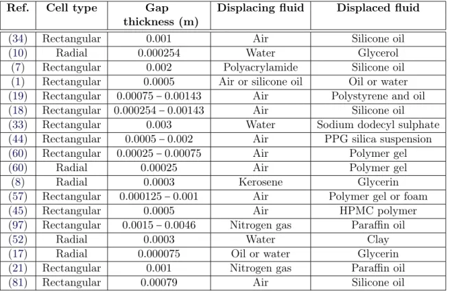
I The characteristics of Hele-Shaw cell and type of fluids in the literature.. . . . 2 1.1 The ranges and values of the dimensional parameters in our work. The reported

viscosity values correspond to the shear rates between0.12 and 518 (1/s). . . . 36 1.2 The ranges and values of the dimensionless parameters in our work. . . 36 1.3 Carbopol composition and determined parameters from rheological

measure-ments, assuming the Herschel-Bulkley model. . . 40 1.4 Important dimensionless groups that the present study has delivered. . . 61 2.1 The ranges and values of the dimensional parameters in our work. ∗_{A number}

of additional experiments have been also performed in a cell with a larger gap thickness, ˆb= 2.5 (mm), to enable the cell side-view visualization. ∗∗_For

conve-nience in this work, interfacial tension refers to both liquid-liquid interfacial

tension or liquid-air surface tension.. . . 73 2.2 The ranges and values of the dimensionless parameters in our work. . . 74 2.3 Carbopol composition, parameters determined from rheological measurements

(assuming the Herschel-Bulkley model), and static contact angles for a Carbopol drop in oil (θoc) and for a Carbopol drop in air (θac), in contact with an acrylic

plastic substrate. . . 77 2.4 The logic notations used in our work to present results. . . 84 2.5 B¯2 (i.e., the mean value of ¯B2 for different velocities) of for oil and air

displace-ments for given values of the channel thickness and the Carbopol concentration. 111 2.6 Important critical dimensionless groups for wetting (oil-Carbopol)

displace-ment that the present study has delivered, in comparison with non-wetting (air-Carbopol) displacements. Some dimensionless group values for non-wetting

(air-Carbopol) displacements are from (36). . . 114 4.1 Definitions and ranges of the dimensionless parameters used in this manuscript.

Here, ˆV0 is the mean imposed velocity. In the definition of the Reynolds number,

ˆ

ν = ˆηH/ˆρ with ˆηH being the viscosity of the heavy fluid and ρˆ= (ˆρL+ ˆρH)/2.

In the definition of the Péclet number, ˆDm is the molecular diffusivity. m is 1

everywhere, unless otherwise stated. Hereafter, the densimetric Froude number,

denoted byF r, is called the Froude number for convenience. . . 142 4.2 Summary of the main observations. . . 169

(10)

List of figures

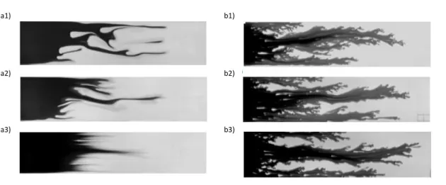
I Various viscous fingering patterns in Hele-Shaw cells. (a) Miscible Newtonian fluid in a radial geometry (10). (b) Immiscible Newtonian fluid in a vertical cell

(62). (c) Miscible non-Newtonian fluid in a horizontal rectangular cell (88). . . 4 II Miscible viscous fingering when dyed water displaces glycerin in a Hele-Shaw

cell. (a)q= 0.002 ml/s, (b) q = 0.00054 ml/s and (c) q = 0.00014 ml/s. Immiscible viscous fingering when dyed oil displaces glycerin in a Hele-Shaw cell. (d) q =

0.002 ml/s, (e) q= 0.00054 ml/s and (f) q = 0.00014 ml/s (16). . . 7 III Schematic view of the propagation of a single finger in a Hele-Shaw cell which

produces a film behind the finger (84). . . 8 IV Experimental snapshots of viscous fingering∶ (a) Uniform cell and (b)

Conver-ging cell (84). . . 10 V Response to stress relaxation test where a shear strain is suddenly applied on

materials (42). . . 13 VI Viscous fingering pattern in a Hele-Shaw cell. (a) Newtonian fluid at low

ve-locity. (b) Newtonian fluid at high veve-locity. (c) Non-Newtonian fluid at low

velocity (90). . . 14 VII Experimental snapshots of the viscous fingers∶ (a) low velocities and (b) high

velocity. (c) The variation of finger width versus finger velocity for yield stress

fluid (57; 58). . . 15 VIII Displacement of Alcoflood solutions by water for weakly shear-thinningn= 0.85

with injection rate of (a1) 0.431 ml/min, (a2) 2.168 ml/min and (a3) 10.790 ml/min. Displacement of Alcoflood solutions by water at flow rate rate 2.168 ml/min for strongly shear-thinning (b1)n= 0.59, (b2) n = 0.57 and (b3) n = 0.49

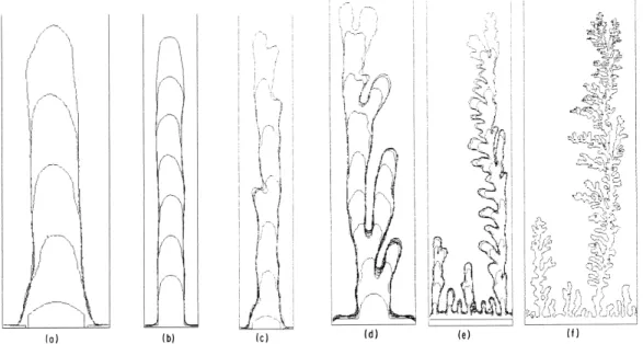
(53). . . 17 IX Example of typical patterns for viscoelastic fluids. For each row, the injection

rate increases from low value on the left to high value on the right. The first two rows are for the high molecular weight (concentrations are 0.3 wt% and 0.8 wt%, respectively). The last two rows are for the low molecular weight (concentrations are 5 wt% and 10 wt%, respectively). ˆb= 0.4 mm for all cases except for the first row where ˆb= 0.8 mm. The numbers in the graph indicate

the injection rates in (ml/min) (98). . . 18 X Concentration fields for differentRe∗ _(95). _{. . . .} ₂₁

XI The effect of the Bingham number on the shape of the finger shape atΓ= 0.002

(upper row) and at Γ= 0.0004 (lower row) (27). . . 21 XII The different pattern formations as a function of surface tension. (a) 1/B = 35,

(b)1/B = 46, (c) 1/B = 104, (d) 1/B = 208, (e) 1/B = 2083 and (f) 1/B = 16666

(11)

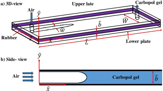
1.1 Schematic view of the experimental set-up (i.e., a rectangular Hele-Shaw cell).

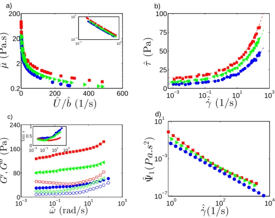
(a) A 3D-view of the geometry and the flow. (b) Side view.. . . 37 1.2 Various rheology results for experiments with LCC (●), MCC (▸) and HCC (∎).

(a) Viscosity (ˆµ) as a function of the shear rate ( ˆU/ˆb) based on equation (1.4). The inset shows the same data as in the main graph but with a logarithmic scale. (b) Flow curves of the shear stressτ versus the shear rate ˆ˙ˆ γ. The dashed lines correspond to the Herschel-Bulkley model parameters fitted to data. (c) The storage modulus (filled symbols) and the loss modulus (hollow symbols) as a function of frequency (ˆω). The inset shows the loss factor versus frequency.

(d) The first normal stress coefficient ( ˆΨ1) as a function of the shear rate.. . . 39

1.3 Experimental results of the displacement of an MCC gel by air in a Hele-Shaw cell geometry with ˆb = 0.9 (mm). (a) Experimental images of the displace-ment flow. The air flows from left to right. Effects of increasing the mean imposed velocity ( ˆV ) on the finger patterns can be seen. The mean impo-sed velocities are ˆV = 0.58, 6.3, 31.4 (mm/s) and the finger tip velocities are

ˆ

U = 2.4, 30.2, 147.5 (mm/s), from top to bottom. The field of view for each of these snapshots is4.7× 21.3 (cm2). (b) Variation of the finger width, w, versusˆ the finger tip velocity, ˆU . Three different flow regimes are marked by ∎ (yield stress regime), ▸ (viscous regime), and ☀ (elasto-inertial regime). The arrow indicates the transition point where inertial effects start to become important.

The inset shows the same data as in the main graph but with a linear scale. . 42 1.4 Variation of the finger width versus the finger tip velocity∶ (a) The results are

shown for three Carbopol concentrations and a fixed channel thickness (ˆb = 1.5 (mm)). The data correspond to experiments with LCC (◻), MCC (⊛) and HCC (☀). (b) The results for two different channel thicknesses and a fixed MCC. The data correspond to experiments with ˆb = 1.5 (mm) (⊛) and ˆb = 0.9 (mm) (◂). The insets are the same as the main graph but with a semi-log

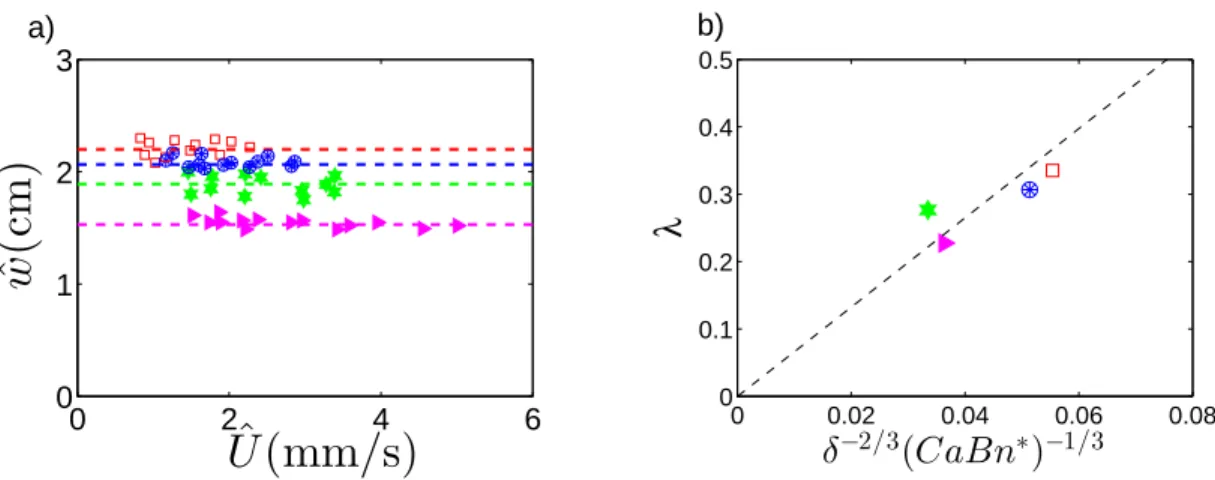
x-axis, where the three regimes are more visible. . . 43 1.5 Results for the yield stress regime with the following experimental parameters∶

ˆb = 1.5 (mm) & LCC (◻), ˆb= 1.5 (mm) & MCC (⊛), ˆb= 1.5 (mm) & HCC (☀), and ˆb= 0.9 (mm) & MCC (▸). (a) Variation of the finger width versus the finger tip velocity. The horizontal dashed lines show the mean values ofw for all ˆˆ U in this regime. These mean values are used for plotting the subfigure on the right. (b) The dimensionless mean value of finger width (λ= ˆw/ ˆW ) as a function of δ−2/3(CaBn∗)−1/3

. . . 44 1.6 Finger width versus various parameters for ˆb = 1.5 (mm) & LCC (▲), ˆb =

1.5 (mm) & MCC (●), ˆb= 1.5 (mm) & HCC (∎), and ˆb= 0.9 (mm) & MCC (☀). (a) w versus ˆˆ U . The dashed lines are fitted curves as eye guides. (b) λ versus Ca δ1+n_{, showing the collapse of two data sets (different channel thicknesses)}

onto a single curve. In the top & bottom insets, the exponents of δ are 1 and 2, respectively. (c) λ as a function Ca δ1+n, showing the collapse of 4 data sets (different Carpool concentrations) onto a single curve. (d) Values of the Bingham number Bn (indicated by size and by the color in the color bars),

(12)

1.7 (a) λ as a function of Ca δ1+n_{/Bn. The dashed lines are fitted curves as eye}

guides. The vertical solid lines indicate the transition points at which λ starts to decrease, for each experimental sequence of increasing velocity (on average Ca δ1+n_{/Bn ≈ 550). The data correspond to the experiments with ˆb = 1.5 (mm)}

& LCC (∎), ˆb = 1.5 (mm) & MCC (●), ˆb = 1.5 (mm) & HCC (☀), and ˆb = 0.9 (mm) & MCC (◂). (b) Different flow regimes observed in the plane of Ca δ1+n _and _{Bn. The symbols correspond to the yield stress regime (}_∎_),

the viscous regime (●), and the elasto-inertial regime (☀). The oblique da-shed line indicates the transition between the yield stress and viscous regimes (Ca δ1+n/Bn = 550). The vertical dashed line at Bn = 0.5 separates the data corresponding to the viscous and elasto-inertial regimes. The yield stress and viscous regime data points from the literature are also superposed. The symbols correspond to the yield stress regime (hollow symbols) and the viscous regime

(filled symbols). The data are from (43) (▼,▽), (21) (▸,▷) and (46) (▲,△).. . 47 1.8 Results for the elasto-inertial regime with the following experimental parameters∶

ˆb = 1.5 (mm) & LCC (◻), ˆb= 1.5 (mm) & MCC (⊛), ˆb= 1.5 (mm) & HCC (☀), and ˆb= 0.9 (mm) & MCC (◂). (a) The finger width as a function of the finger tip velocity. (b) Superposition of the experimental data when 1/λδ1+n _{is used.}

The dashed line shows a plateau value of1/λδ1+n_{= 0.026.} _{. . . .} ₄₈

1.9 The dimensionless finger width as a function different dimensionless groups for data at different aspect ratios and Carpool concentrations∶ (a) λ as a function W e∗_{. (b)}_{λ as a function Ca δ}1+n_{. (c)}_{λ as a function Ca}∗_{. The data correspond}

to experiments with ˆb = 1.5 (mm) & LCC (▲), ˆb = 1.5 (mm) & MCC (●),

ˆb = 1.5 (mm) & HCC (∎) and ˆb = 0.9 (mm) & MCC (☀). . . 50 1.10 The regimes classification based on elastic properties. Viscoelastic regime (☀)

and inelastic regime (▲). The vertical dashed line shows W i= 0.13, which is

roughly the transition to elasto-inertial regime. . . 51 1.11 An experimental snapshot showing the movement of the finger side due to an

elastic response. The right image is zoomed-in on the indicated box of the left image. The red color indicates the displacing fluid (air) and the black color shows the displaced fluid (Carbopol). The dark red color shows the oscillation of the Carbopol layer within ˆt= 0.358 − 0.4 (ms). The images show the field of

view of5.8× 17.5 (cm2_{) (left) and of}_4.3_{× 1.25 (cm}2_{) (right).}_{. . . .} ₅₂

1.12 The oscillation in the local finger width due to elastic response at different times with respect to the beginning of the experiment. The dashed line is smoothing

spline fitted curve. . . 52 1.13 Results for experimental data corresponding to ˆb = 1.5 (mm) &LCC (▸), ˆb =

1.5 (mm) & MCC (●), ˆb= 1.5 (mm) and HCC (∎), and ˆb= 0.9 (mm) & MCC (☀). (a) Thickness of wetting film (t) as a function of Ca. (b) Variation of Bn in the plane oft and Ca. The colors/symbol sizes illustrate the magnitude of Bn. (c) Variation oft versus Bn. The dash-dot line shows hcirc from equation (1.11),

i.e., when Ca→ ∞. (d) Comparison between the experimental and theoretical prediction (equation (1.14)) of the wall layer thickness. The dashed line shows

(13)

1.14 An experimental snapshot (top view) showing 4 sequential steps of the process of the network structure formation within the finger domain. The experimental times are 1326, 1353, 1393, 1473 (ms), from top to bottom. The mean imposed velocity is ˆV = 34.6 (mm/s) (the finger tip velocity is ˆU = 315.3 (mm/s)). The images correspond to the experiment with ˆb= 0.9 (mm) & LCC. The field of

view for these snapshot is22.8× 5.6 (cm2_). _{. . . .} ₅₆

1.15 (a) Schematic view of a probable 4-stage process of the formation of network structure regime (side channel view). (b) Schematic view of the intermediate stage of the network structure formation, as the residual layer breaks up into

several pieces. . . 57 1.16 (a) Variation in the total number of cavities (∎) and the mean characteristic

diameter of cavities (▲) versus time, in the network structure regime, for the same experiment as in Fig. 1.14. (b) Variation in relative mean light intensity versus length of cell for 4 sequential images of Fig. 1.14. (c) Variation in mean

light intensity of cavities (●) and Carbopol pieces (▲) versus time. . . 59 1.17 Image sequence showing the finger evolution in the network structure regime.

Different areas are explained in the text. . . 60 1.18 A secondary flow regime classification based on the formation of a network

structure inside the finger domain. The data correspond to the experiments for the network structure regime are marked by☀and the ones without by●. The

black dashed line indicates transition between the two regimes∶ Ca = 0.86Bn−2.82. 60 2.1 (a) A 3D schematic view of the experimental set-up, showing our rectangular

Hele-Shaw cell and the flow within. (b) A schematic side-view of oil displacing Carbopol (with a concave interface). (c) A schematic side-view of air displacing

Carbopol (with a convex interface). Note the film of Carbopol left on the walls. 76 2.2 (a) Flow curves of shear stress, τ , versus shear rate, ˆ˙ˆ γ. The lines correspond

to the Herschel-Bulkley model parameters fitted to data. (b) First normal stress difference ( ˆN1) as a function of ˆ˙γ. The solid lines show the power-law fit corresponding to HCC ( ˆN1 = 1.35ˆ˙γ 0.55 ), MCC ( ˆN1 = 1.09ˆ˙γ 0.52 ) and LCC ( ˆN1= 0.58ˆ˙γ 0.51

). The inset presents the same data as in the main graph but in a logarithmic scale. The dash-dot line shows the variation of ˆN1 as a function of ˆ˙γ based on equation (2.8). (c) Relaxation time, ˆΛ, as a function of the cha-racteristic shear rate ( ˆU/ˆb) based on equation (2.11). The data correspond to

HCC (●), MCC (∎) and LCC (▲). . . 79 2.3 Wall contact angle of a small drop of Carbopol (MCC) placed on an acrylic

plastic plate submerged in an oil-filed reservoir (left) and in an air-filled reservoir

(right). The field of view for each snapshot is5.5× 3.4 (mm2). . . 80 2.4 Variation of the wall contact angle of a small drop versus time. The data

corres-pond to experiments with oil-Carbopol (HCC) (●), oil-Carbopol (LCC) (●), air-Carbopol (HCC) (◻) and air-Carbopol (LCC)(◻). MCC results are not shown

(14)

2.5 Experimental results of the displacement of an LCC gel by (a) oil and by (b) air, in a Hele-Shaw cell geometry with ˆb = 1.5 (mm). The oil/air flows from left to right. In both (a) and (b), the mean imposed velocities are ˆV = 0.09, 0.3, 5.7, 29 (mm/s), from top to bottom. The field of view for each snap-shot is6.12×22.05 (cm2). (c) Variation of the finger width,w, versus the fingerˆ tip velocity, ˆU . Different flow regimes are marked∶ capillary (☀); yield stress (●,○); viscous (▲,△), and elasto-inertial (∎,◻). Note that the capillary regime is not observed for air-Carbopol displacements. The vertical solid (dashed) lines show transition boundaries for oil-Carbopol (air-Carbopol) displacements. The solid (dashed) arrow indicates the critical point where inertial effects start to

become important, for displacements of Carbopol gel by oil (air). . . 86 2.6 (a) Variation of w versus ˆˆ U , for different channel thicknesses and at a fixed

Carbopol concentration, MCC. The data correspond to experiments with ˆb= 0.9 (mm) (●, ○) and ˆb= 1.5 (mm) (☀, ☆). The channel thickness in wetting (non-wetting) displacement flows increases in the solid (dashed) arrow direction. (b) Variation ofw versus ˆˆ U , for different Carbopol concentrations and at a fixed channel thickness, ˆb= 1.5 (mm). The data correspond to experiments with LCC (◂, ◁), MCC (☀, ☆), HCC (⊛, ○). The Carbopol concentration in wetting

(non-wetting) displacement flows increases in the solid (dashed) arrow direction. 88 2.7 Experimental side-view snapshots showing the interface shape for HCC in a cell

with ˆb= 2.5 (mm) for air-Carbopol (left) and oil-Carbopol (right) displacements. The field of view in each snapshot is3.94× 18.63 (mm2_{). The oil/air flows from}

left to right. The mean imposed velocity is ˆV ≈ 0.04 (mm/s), in both cases. . . 89 2.8 Oil-Carbopol interface evolution, from side-view, versusCa at a given channel

thicknesses (ˆb = 2.5 (mm)) and a fixed Carbopol concentration, HCC. The capillary numbers are Ca = 0.78, 0.86, 0.92, 0.97, 1.04, from left to right. The

field of view in each snapshot is3.94× 12.93 (mm2_{). . . .} ₉₀ 2.9 Variation oftan θd versus (a)Ca and (b) Bn at a given channel thickness (ˆb=

2.5 (mm)) for oil-Carbopol displacements. The data correspond to experiments with HCC (●) and MCC (∎). In (a) the solid lines present the theoretical results

of equation (2.16) and equation (2.17) for Newtonian fluids. . . 92 2.10 (a) & (b) Variation of w versus ˆˆ U in the capillary regime, for oil-Carbopol

displacements. The data correspond to experiments at ˆb= 0.9 (mm) with LCC (∎), MCC (●) and HCC (▲) and at ˆb= 1.5 (mm) with LCC (◂), MCC (☀), HCC (⊛). The horizontal lines show the mean values ofw. Note that in air-Carbopolˆ

displacements, the capillary regime is not observed. . . 92 2.11 (a) & (b) Variation of w versus ˆˆ U in the yield stress regime, for oil (filled

symbols) and air (hollow symbols). The horizontal lines and dashed lines show the mean values ofw. The data correspond to experiments at ˆbˆ = 1.5 (mm) with LCC (◂, ◁), MCC (☀, ☆), HCC (⊛, ○) and at ˆb= 0.9 (mm) with LCC (∎), MCC (●,○) and HCC (▲). (c) Dimensionless mean finger width,λ, as a function of a dimensionless control parameter,λ= c_ˆ

W

√

ˆ σˆb ˆ

τy, withc being the coefficient of

the linear fit. Our wetting displacement results (∎) against non-wetting results

(15)

2.12 (a) Variation of λ versus Caδ1+n_{, at different Carbopol concentrations, with}

three data sets of oil-Carbopol and three data sets of air-Carbopol displacement results. The data correspond to experiments at ˆb= 1.5 (mm) with LCC (◂,◁), MCC (☀,☆), HCC (⊛,○). (b) λ as a function ̃Caδ1+n_{, with the same}

para-meters as in (a), showing a collapse of data for oil-Carbopol and air-Carbopol displacements. (c) λ as a function ̃Caδ1+n_{, with various Carbopol}

concentra-tions and channel thicknesses, for six data sets of wetting displacements (filled bullets) and four data sets of non-wetting displacements (hollow squares). The

change in Bn is illustrated by the size and color. . . 97 2.13 (a) & (b) Variation ofw versus ˆˆ U in the elasto-inertial regime in wetting

displa-cements. (c) Superposition of experimental data for wetting and non-wetting displacements at large ˆU when 1/λδ1+n _{is used. The line marks the plateau}

value (1/λδ1+n _{= 0.014) for oil and the dashed line marks the plateau value}

(1/λδ1+n= 0.026) for air. The data correspond to experiments at ˆb = 1.5 (mm) with LCC (◂, ◁), MCC (☀,☆), HCC (⊛,○) and at ˆb= 0.9 (mm) with LCC

(∎), MCC (●,○) and HCC (▲). . . 99 2.14 λ as a function of W e∗

. The data correspond to experiments at ˆb = 1.5 (mm) with LCC (◂, ◁), MCC (☀,☆), HCC (⊛,○) and at ˆb= 0.9 (mm) with LCC (∎), MCC (●,○) and HCC (▲). The solid (dashed) line shows the critical mo-dified Weber numberW e∗

c ≈ 1480 (We ∗

c ≈ 76.5) for oil-Carbopol (air-Carbopol)

displacement flows. . . 100 2.15 The dimensionless finger width as a function of different dimensionless groups

for data at different aspect ratios and Carpool concentrations∶ (a) λ as a function of ̃Caδ1+n. (b) λ as a function of ̃Ca∗. (c) λ as a function of At× ̃Ca∗. (d) λ as a function ofCaδ2_._{The inset shows the same data as in the main graph but} a logarithmic scale. The data correspond to experiments at ˆb= 1.5 (mm) with LCC (◂, ◁), MCC (☀, ☆), HCC (⊛, ○) and at ˆb= 0.9 (mm) with LCC (∎),

MCC (●,○) and HCC (▲). . . 101 2.16 (a) Four different flow regimes observed in wetting displacements, in the plane

of Caδ1+n and Bn. (b) The yield stress and capillary regimes in the plane of Ca and θd. The horizontal line at θd ≈ 90○ separates the data

correspon-ding to the capillary and yield stress regimes. Note that the capillary regime is not observed for non-wetting displacement flows. (c) The viscous and yield stress regimes, for wetting flows (filled symbols) and non-wetting flows (hollow symbols), in the plane of Caδ1+n _and _{Bn. The transition between the yield}

stress and viscous regimes is marked by the oblique solid (dashed) line for oil-Carbopol (air-oil-Carbopol) displacements, for which slope is Caδ1+n_{/Bn = −1050}

(Caδ1+n_{/Bn = 550). Neglecting the small dependency on Caδ}1+n_{, the transition}

for wetting flows (non-wetting flows) occurs roughly at Bnc≈ 1 (Bnc≈ 1.25).

The symbols correspond to the capillary (▲), yield stress (∎,◻), viscous (●,○), elasto-inertial (☀,☆) regimes. In (d), inelastic flows (including the capillary, yield stress and the viscous regimes) are marked by (⧫,◊). In (d), for wetting (non-wetting) displacements, the vertical solid (dashed) line marks W ic= 0.33

(16)

2.17 A schematic side-view of oil displacing Carbopol with (a) a concave interface and (b) a convex interface. A typical variation in the relative mean light intensity versus length of cell for (c) a concave interface and (d) a convex interface. The upper insets show the same data as in the main graphs but for a longer cell length. The corresponding experimental snapshots (as lower insets) show the displacement of HCC Carbopol gel by oil in a cell with ˆb= 0.9 (mm). The oil flows from left to right. The field of view in each snapshot is 6.03× 23.3 (cm2_). The solid line and dashed line passing in the middle of the cell mark where the

relative mean light intensities are calculated. . . 105 2.18 (a) Variation of tan θd versus Ca in the capillary regime, estimated using the

indirect approach (i.e., analyzing the variation of ¯I). The datapoints (☀) from the direct measurement (from Fig.2.9a) are also superposed. (b) Variation ofθd as a function ofCa. The symbols correspond to the yield stress regime (square symbols) and the capillary regime (triangle symbols). The data correspond to experiments at ˆb= 0.9 (mm) with LCC (▲,∎), MCC (▲,∎), HCC (▲,∎) and at ˆb= 1.5 (mm) with LCC (▲,∎), MCC (▲,∎) and HCC (▲, ∎). The lines in subfigure (b) are fitted curves (as eye guides) for each set of experiments. The

horizontal dashed line showsθd= 90○. . . 106 2.19 Experimental results of the displacement of (a) MCC Carbopol gel and (b)

Xanthan gum solution, by oil in a cell with ˆb= 1.5 (mm). The oil flows from left to right. The mean imposed velocity is ˆV ≈ 0.11 (mm/s), in both cases. The field of view in each snapshot is 6.6× 21.3 (cm2_{). (c) Flow curves of shear}

stress,τ , versus shear rate, ˆ˙ˆ γ for the MCC Carbopol gel (∎) in comparison with the Xanthan gum solution (☀). The lines correspond to the Herschel-Bulkley

model parameters fitted to data.. . . 107 2.20 Variation of λ as a function of Ca for the displacement of HCC Carbopol gel

and Glycerol solution, by oil in a cell with ˆb= 0.9 (mm). The data correspond

to experiments with HCC (▲) and Newtonian fluid (oil-Glycerol) (☀). . . 107 2.21 Experimental snapshots showing the oscillation of the finger side due to

secon-dary instabilities in the elasto-inertial regime (top view xˆˆz-plane). The finger upper half is shown. (a) Oil displaces Carbopol gel, from left to right. (b) Air displaces Carbopol gel, from left to right. The field of view of3.36×24.05 (cm2) in both images. The red solid (dashed) curve shows the result of applying equa-tion (2.27) for the oil (air) flow. Note that here the origin of thez-axis is shiftedˆ

to the cell middle. . . 109 2.22 (a) A2 versusW e∗ for oil-Carbopol displacements. (b) A2 versus W e∗ for

air-Carbopol displacements. In (a&b), the data correspond to experiments at ˆb= 1.5 (mm) with LCC (◂,◁), MCC (☀,☆), HCC (⊛, ○) and at ˆb= 0.9 (mm) with LCC (∎), MCC (●,○) and HCC (▲). (c&d)B2 in the plane ofW i, Bn and

Caδ1+n _{for (c) oil and (d) air displacements. The values of} _B

2 are marked by

the symbol size and colors. The lines in (a&b) are fitted curves (as eye guides)

(17)

2.23 Orientation of side branches for (a) wetting and (b) non-wetting displacements. The oil/air flows from left to right. For oil (air), the peak heights and the peak widths at half height are shown by the brown vertical solid (dashed) lines and the green horizontal solid (dashed) lines, respectively. For oil (air), each peak is marked by▼(▽) while the center of each peak width at half height is marked by ∎ (◻). For oil (air), each peak angle, β, is defined using the slope of the oblique solid (dashed) line, passing through the peak and the peak width at half height. Note that any peak whose height is smaller than 1 (mm) is filtered. Also note that here the origin of the z-axis is shifted to the cell middle. Bothˆ

images show a field of view of2.95× 21.53 (cm2_)._{. . . .} ₁₁₃

2.24 (a) Comparison among ¯βoiland ¯βairfor wetting and non-wetting displacements,

respectively, with the same experimental conditions (i.e., same channel thick-ness, imposed flow velocity, and Carbopol concentration). The values ofW i are marked by the symbol size and colors. Dashed line shows ¯βoil= ¯βair. (b) ¯β (the¯

mean value of ¯β for different imposed velocities) for oil and air displacements at (i) ˆb= 1.5 (mm) with HCC; (ii) ˆb = 1.5 (mm) with MCC; (iii) ˆb = 1.5 (mm)

with LCC; and (iv) ˆb= 0.9 (mm) with MCC. . . 114 3.1 A 3D schematic view of the experimental set-up∶ air is injected into Carbopol

gel. The imposed velocity is determined by an Alicat mass flow controller. Also for recording the finger behaviours, a Basler high speed camera mounted on top

of the cell is used. . . 126 3.2 Flow curves of shear stress, τ , versus shear rate, ˆ˙ˆ γ. The lines correspond to

the Herschel-Bulkley model parameters fitted to data. The data correspond to high Carbopol concentration (⧫)(ˆτ = 13.7 + 11.6 ˆ˙γ0.35_{) and low Carbopol}

concentration (▲)(ˆτ = 5.4 + 5.7 ˆ˙γ0.32_)._{. . . .} ₁₂₇

3.3 Diagram of the different flow patterns as a function of the gap thickness, the channel width and the imposed velocity at the low Carbopol concentration. The

air flows from left to right. . . 128 3.4 (a) Two different flow patterns observed, in the plane of Bo∗ _and _{ET . The}

symbols correspond to the branched fingering patterns (●) and the single finger patterns (○). The horizontal line (ab) at ET ≈ 0.45 and the vertical line (bc) at Bo∗ ≈ 0.02 separate the data corresponding to the two patterns. The single

and branched fingering flow data points from the literature are also superposed. The symbols correspond to the single finger (hollow symbols) and the branched fingering (filled symbols). The data are from (20) (▸,▷), (19) (⧫,◊), (24) (△) and (25) (◻). Several experimental snapshots corresponding to the branched fingering and single finger patterns are presented in (b) and (c). Subfigures (b) and (c) show the effect ofBo∗_{(above critical}_{ET ) and ET on the flow patterns,}

respectively. The lines (bc) and (ab) represent the same lines as the main graph

(18)

3.5 λ as a function Caδ1+n _{for data at different channel widths, gap thicknesses}

and Carpool concentrations. The data correspond to experiments with both low and high Carbopol concentrations at various δ= W (mm)ˆ_ˆ

b (mm) ∶ 4.5 3 (△), 6 3 (◻), 9 3 (☀), 12₃ (●), 15₃ (∗), 21₃ (▼), 30₃ (☀), 36₃ (●), 45₃ (◂), 60₃ (∎), 130₃ (☀), _0.260 (⧫), 60 0.3 (∗), 60 0.5 (◁), 60 1 (☆), 60 1.5 (▽), 60 2.1 (○), 60 4.33 (△), 60 5.5 (◊), 20 0.9 (☆), 25 0.9 (∗), 68 1.5

(◻) and _1.540(▼). The datapoints seem to follow a solid red curve indicated by λ= 2.82 (Caδ1+n₎−0.46_{. The inset shows Newtonian results from the literature}

in the plane ofλ and Caδ1+n(for Newtonian fluids the control parameter turns intoCaδ2_{). The results are from (12)(δ}_{= 65 (}_●_{)), (15) (δ}_{= 1 (}_▼_),_δ_{= 1.99 (}_▲_),

δ = 6 (⧫)). The theoretical results of (11) are shown using the black dashed

curve. The red solid line is the same as the one in the main graph. . . 131 4.1 Schematic view of the numerical domain (a) at the initial flow configuration

and (b) after the onset of displacement flow. . . 141 4.2 (a) Evolution of 1− ¯C(t)

1− ¯C(0)versus time for different mesh sizes forBn= 100, Re = 50

andF r= 1000. (b) Evolution of the position of the displacing front, xf ront,

ver-sus time for different mesh sizes for the same simulation. (c)&(d) Concentration colormaps at t= [0, 10, ..., 40] for Bn = 5, Re = 200 and Fr = 0.5 for the mesh

size (c)1500× 42 and d) 2100 × 34. The domain size shown is 1 × 100. . . 143 4.3 Code benchmarking∶ (a) The average static residual wall layer thickness, have=

(hu+ hl)/2, from our simulation (◻) at Re = 100 and Fr = 1000 against the

results of (61) (●) for Re = 100 and Fr = ∞. (b) Concentration colormaps of the displacement flow at timest= [0, 7, ..., 28] for Bn = 10, Re = 100, m = 2 and F r = 7.071. The last image at the bottom of the subfigure is the colorbar of the concentration values (here and elsewhere). The white broken lines display the position of the initial interface x = 0 (here and later). The domain size shown is 1× 100 (unless otherwise stated). The images in this subfigure can be qualitatively compared with Fig. 2 in (51). To validate the code against the results of Swain et al. (51), we have exceptionally considered a light-heavy

displacement flow. . . 144 4.4 Panorama of concentration colormaps at t= 16 and Re = 400 for (a) Fr = 0.5

and (b) F r= 100. The rows from top to bottom show Bn = 0, Bn = 2, Bn = 5,

Bn= 20, Bn = 50, Bn = 100, Bn = 200. The domain size shown is 1 × 60.. . . . 145 4.5 Computational results for Bn = 50, Re = 500 and Fr = 1; (a) Concentration

colormaps at times t = [0, 10, ..., 40]; (b) Shear stress colormaps at times t = [0, 10, ..., 40]; (c) Interface heights (lower and upper layers) at t = 40∶ hu and

hl show the thickness of upper and lower static layers, respectively. The red

arrows indicate the position at which uniform static layers appear, with xu

indicating the upper static distance andxl the lower static distance. (d) Speed

contours∶ V = √

Vx2+ Vy2. (e) Velocity vectors. (f) The image is zoomed-in on

(19)

4.6 Effects ofBn, F r and Re on static residual layer thicknesses∶ (a) hu and (b)hl.

The data correspond to Re= 50 (▸), Re= 100 (∎), Re= 200 (●),Re= 300 (◂), Re= 400 (⋆) andRe= 500 (▼). In this and the following figures, the error-bars (estimated through the standard deviation of the static layer thicknesses) are shown in one graph only, while the error-bars of the other data are more or less similar (not shown). The insets are zoomed at the variation of the lower static

thickness. . . 148 4.7 The upper row shows the variation ofhu(filled symbols) andhl(hollow symbols)

versusF r for different values of Bn at∶ (a) Re = 500; (b) Re = 100; (c) Re = 1. The lower row shows the variation of hu/hl versus F r for∶ (d) Re = 500; (e)

Re= 100; (f) Re = 1. The data correspond to Bn = 2 (▸),Bn= 5 (∎),Bn= 20

(●),Bn= 50 (◂),Bn= 100 (⋆), Bn= 200 (▼).. . . 149 4.8 Comparison among static layer thicknesses from our simulation results (filled

symbols), hcirc (dashed line) and hmax,u or hmax,ave (hollow symbols). The

upper row showshuand the bottom row shows the mean value of the lower and

upper static layer thicknesses (have= hu₂+hl). The data correspond to Re= 100

(∎) and Re = 500 (▲). The insets indicate the ratio of the simulation upper layer thickness to the upper maximal static layer thickness, hu/hmax, versus

Bn for the same datapoints as in the main graphs.. . . 150 4.9 Effects ofBn, F r and Re on (a) xu and (b)xl. The data correspond toRe= 50

(▸), Re= 100 (∎),Re= 200 (●),Re= 300 (◂),Re= 400 (⋆),Re= 500 (▼). The

insets display the same data as in the main graphs but with a linear scale. . . 153 4.10 The ratioxl/xu. In the upper row, the data correspond toRe= 50 (▸),Re= 100

(∎),Re= 200 (●),Re= 300 (◂),Re= 400 (⋆), Re= 500 (▼). In the lower row, the data correspond to F r = 0.5 (▸), F r = 1 (∎), F r = 2 (●), F r = 10 (◂),

F r= 100 (⋆),F r= 1000 (▼). . . 154 4.11 Regime classification based on the class of the slump-type (●) and center-type

(○) regimes. The dashed line represents Re/Fr = 60. Snapshot images belong to Bn = 20, Re = 500, and Fr = 1000 at t = 8.9 (center-type) and Bn = 50,

Re= 500, and Fr = 2 at t = 12.7 (slump-type). . . 154 4.12 Concentration colormaps at t = [0, 8, ..., 32] for (a) Bn = 200, Re = 100 and

F r= 0.5 (a case without a back flow) and (b) Bn = 2, Re = 500 and Fr = 0.5 (a case with a back flow). (c) & (d) Spatiotemporal diagrams of the depth-averaged concentration values for the same simulations as in (a) & (b). The size of the

domain shown is 1× 76, starting from before the gate valve at x = −12.. . . 156 4.13 Flow regime classification based on appearing back flows. The data

correspon-ding to the temporary-back-flow regime are marked by (●) and the no-back-flow regime by (○). Snapshot images belong to Bn= 2, Re = 400, and Fr = 0.5 at t= 7.3 (temporary-back-flow) and Bn = 50, Re = 500, and Fr = 1 at t = 10.6 (no-back-flow). The broken red arrow indicates the location of trailing front.

The domain size shown is 1× 60.. . . 157 4.14 Concentration colormaps and velocity vectors at t = [6.8, 13.85, ..., 35] for (a)

Bn= 5, Re = 200 and Fr = 0.5 and (b) Bn = 5, Re = 500 and Fr = 10, showing two types of unstable displacements. The domain size shown is1× 57, starting

(20)

4.15 Concentration colormaps and velocity vectors, at t = [4, 6, 8, 10, 14, 19, 26] for Bn= 100, Re = 300 and Fr = 0.2, showing 7 sequential steps in a displacement flow with periodic detachment. The domain size shown is 1× 50, starting from

the gate valve position atx= 0. . . 158 4.16 Colormaps of (a) concentration, (b) stress (second invariant of the deviatoric

stress) and (c) shear stress, as well as (d) velocity vectors, at t = [13] for Bn = 100, Re = 300 and Fr = 0.2, showing a displacement flow with periodic

detachment. The domain size shown is1× 18, starting from x = 25. . . 159 4.17 The mean characteristic diameter of detached segments ( ¯d) at F r = 0.1; (a)

versus Re with the data corresponding to Bn = 2 (▸), Bn = 5 (∎), Bn = 20 (●), Bn = 50 (◂), Bn = 100 (⋆), Bn = 200 (▼); (b) versus Bn with the data corresponding to Re = 50 (▷), Re = 100 (◻), Re = 200 (●), Re = 300 (◁), Re = 400(⋆), Re = 500 (▽). ¯d is calculated using ¯d = √4A_π , where A is the

segment area. . . 160 4.18 Flow regime classification based on stable/unstable flows. The stable datapoints

are marked by (○) and the unstable ones by (●). Two snapshots corresponding to a stable flow (Bn= 100, Re = 500, and Fr = 1 at t = 32) and an unstable flow (Bn = 5, Re = 50, and Fr = 0.35 at t = 40) are included. Within the unstable displacement flows, the ones with the periodic-detachment patterns are marked by (◻), the semi-detached patterns by (▽) and the sinusoidal shaped wave

patterns by (△). . . 161 4.19 Classification of front patterns∶ plug-like (○), inertial tip (●), semi-detached (◁)

and fully-detached (⋆). Four snapshots corresponding to a plug front pattern (Bn = 100, Re = 200, and Fr = 1 at t = 35), inertial tip pattern (Bn = 20, Re= 100, and Fr = 0.35 at t = 28), semi-detached pattern (Bn = 20, Re = 300, andF r= 0.5 at t = 20) and fully-detached front pattern (Bn = 2, Re = 300, and

F r= 0.35 at t = 16) are included. . . 162 4.20 (a) & (b) Concentration colormaps and velocity vectors at t= [3.5, 7.2, ..., 22]

for (a) Bn = 50, Re = 400 and Fr = 100 and (b) Bn = 200, Re = 500 and F r= 0.5, showing two examples of the plug-like front. The domain size shown

is1× 40, starting from the gate valve position at x = 0. . . 163 4.21 Concentration colormaps and velocity vectors att= [3, 6.25, ..., 16] for∶ (a) Bn =

20, Re= 100 and Fr = 0.5 and (b) Bn = 2, Re = 400 and Fr = 1, showing two examples with an inertial tip pattern. The domain size shown is1× 44, starting

from the gate valve position at x= 0. . . 164 4.22 (a) Concentration colormaps and velocity vectors, att= [0, 2.5, ..., 10] for Bn =

100, Re = 300 and Fr = 0.1, showing a front detachment configuration. The domain size shown is1× 60, starting from x = −25. (b) Evolution of the leading

(●) and trailing (∎) front velocities for the same simulation. . . 165 4.23 Simulation results at t = 10, for Bn = 50, Re = 200 and Fr = 0.2, showing

a detachment configuration∶ (a) Concentration colormaps; (b) Speed contours V = (√Vx2+ Vy2); (c) Vorticity contours (ω =∂V_∂xy −∂V_∂yx). The domain size

(21)

4.24 Effects of the dimensionless groups on the leading front velocity for at (a)&(c) Re= 100 and (b)&(d) Re = 300. In the top row the data correspond to Fr = 0.5 (▸), F r = 1 (∎), F r = 2 (●), F r = 10 (◂), F r = 100 (⋆), F r= 1000 (▼) and in the bottom row toBn= 2 (▸), Bn= 5 (∎), (●)Bn= 20, (◂) Bn= 50, Bn = 100

(⋆), Bn= 200 (▼). . . 167 4.25 Variation of Vf versus Re for (a) F r = 0.5; (b) Fr = 1; (c) Fr = 10; and (d)

F r = 100. The data correspond to Bn = 20 (●), Bn = 50 (◂), Bn = 100 (⋆),

Bn= 200 (▼). . . 168 4.26 Effects ofRe, Bn and F r on Vf, the values of which are marked by the symbol

size and colors. . . 168 5.1 Schematic of (a) the initial flow configuration and (b) the displacement flow

configuration. . . 179 5.2 Panorama of concentration colormaps atβ= 90○_,_{F r}= 1000 and Re = 500 for (a)

Bn= 0 and (b) Bn = 100. The rows from top to bottom show m = 0.01, 1, 100. The domain size shown is1×75. The last image, at the right hand side of (b), is the colorbar of the concentration values (here and elsewhere). The red broken

lines display the position of the initial interfacex= 0 (here and elsewhere). . . 182 5.3 Panorama of concentration colormaps at β = 90○_,_Bn= 5 and Re = 300 for (a)

F r = 0.5 and (b) Fr = 10. The rows from top to bottom show m = 0.01, 1, 50.

The domain size shown is 1× 100. . . 182 5.4 The mean wavelength of the interfacial waves (¯l) at t= 36 as a function of Bn.

(a) At Re = 200 and Fr = 0.2 with the data corresponding to m = 0.01 (◂), m= 0.1 (∎),m = 1 (●) and m= 20 (▲); (b) At Re = 500 and m = 40 with the

data corresponding to F r= 0.1 (○),F r= 0.2 (◻) andF r= 0.4 (△). . . 184 5.5 Computational results for β = 90○_, _Re = 500, Bn = 100 and Fr = 0.8 at (a,

b, c) m = 1 and at (d, e, f) m = 50; (a) & (d) Concentration colormaps at timest= [2, 6.5, ..., 20]; (b) & (e) Speed contours∶ V =√Vx2+ Vy2 at t= 20 (Vx

denotes the stream-wise velocity component and Vy is the depthwise velocity

component); (c) & (f) Velocity vectors and the interface heights at t= 20∶ huand

hlshow the thickness of upper and lower static residual wall layers, respectively.

The domain size shown is1× 50, starting from the gate valve position at x = 0. The bottom image in subfigures (a) & (d) is the colorbar of the concentration

values (here and elsewhere). . . 185 5.6 Flow regime classification based on the class of the slump-type (▲) and

centre-type (▽) regimes for different viscosity ratios. In each subfigure the horizontal dashed line represents (a) Re/Fr = 60, (b) Re/Fr = 60, (c) Re/Fr = 1200, and

(d)Re/Fr = 3000. . . 186 5.7 The variation of the critical values of Re/Fr versus m for the transition

bet-ween slump-type and centre-type displacements in a horizontal channel. Two illustrative snapshots corresponding to a slump-type flow and a centre-type flow

are included.. . . 187 5.8 The effect of Bn on the leading front velocity, Vf, for Re= 200 and Fr = 0.2.

The channel is horizontal in all cases. The data correspond to m= 0.003 (▼), m= 0.01 (∎),m= 1 (⧫),m= 100 (●),m= 400 (▲). The value ofm increases in

(22)

5.9 Variation of Vf versusm at Re= 500 for (a) Fr = 0.1; (b) Fr = 0.4; (c) Fr = 1;

and (d)F r= 10. The data correspond to Bn = 2 (⧫),Bn= 5 (●), Bn= 20 (◂), Bn= 100 (∎) andBn= 400 (☀). The value ofBn increases in the black arrow

direction.. . . 188 5.10 Variation of Vf versus m∗ at Re = 500 for (a) Fr = 0.1 and (b) Fr = 10. The

data correspond to Bn = 2 (⧫), Bn = 5 (●), Bn = 20 (◂), Bn = 100 (∎) and

Bn= 400 (☀). . . 189 5.11 Concentration colormaps at t = [0, 7, ..., 28] at β = 90○

, Re = 500, Bn = 2 and F r = 0.4 for (a) m = 0.01 (a case with a back-flow), (b) m = 1 (a case with a back-flow) and (c) m = 100 (a case without a back-flow). (d), (e) & (f) Spatiotemporal diagrams of the depth-averaged concentration values for the same simulations as in (a), (b) and (c). The size of the domain shown is1×100.

The red/white arrow marks the trailing/leading front position. . . 190 5.12 Panorama of concentration colormaps atβ= 90○

,m= 1 and Re = 500. The rows from left to right show F r = 0.1, 0.4, 1, 10, 1000. The rows from top to bottom

displayBn= 5, 20, 100. . . 190 5.13 Back-flow and no-back-flow regimes in the plane of F r and Re/Bn for (a)

m= 0.01 and (b) m = 400. The data corresponding to the no-back-flow regime are marked by (●) and the back-flow regime by (⧫). The red and blue colored areas mark the back-flow and no-back-flow regimes m = 1. Two illustrative

snapshots corresponding to a back-flow and a no-back-flow are included.. . . . 191 5.14 Concentration colormaps at Re= 300, Bn = 5 and Fr = 0.5 for (a) m = 0.01,

(b) m= 1 and (c) m = 50. The rows from top to bottom show β = 82, 88, 90○

.

The domain size shown is 1× 100. . . 192 5.15 Concentration colormaps at t= [0, 7.5, ..., 30] at Re = 300, Bn = 5, m = 1 and

F r= 0.5 for (a) β = 88○

and (b)β = 82○

, showing different types of back-flows.

(23)

(24)

Acknowledgement

I would like to convey my gratitude and appreciation to all people who have made this disser-tation possible. My deepest gratitude goes first and foremost to my supervisor, Professor Seyed Mohammad Taghavi, for giving me the opportunity to undertake this Ph.D. for his patience, continuous support, encouragement and immense knowledge. As his first student, it definitely was an honor for me to be a part of his research group. During my Ph.D., his guidance and mentoring helped me to significantly improve my skills and in learning the fundamentals of conducting scientific research.

I would like to thank Professor Denis Rodrigue for useful discussions and his invaluable com-ments about the rheology. I am deeply grateful to Professor Ian Frigaard for his generous support and helpful guidance particularly in the simulation part.

I acknowledge all the people at Laval University, especially Jérôme Nöel, Jean-Nicolas Ouellet and Yann Giroux for their outstanding help in the fabrication and modification of different experimental setups. I appreciate Dr. Roozbeh Molllaabbasi and Mr. Sooran Noroozi for their thoughtful remarks that helped me to improve my thesis considerably.

I would like to thank the Discovery Grant of the Natural Sciences and Engineering Research Council (NSERC) and Canada Foundation for Innovation for the financial supports. I am also indebted to Calcul Quebec and Compute Canada for the HPC platform which have made CFD simulation tests possible.

I would like to thank Prof. Kamran Alba and Prof. Ali Roustaei for their guidance in the simulation part at the early stage of this research. My sincere gratefulness to all my friends, an inspiring group of people especially Amin Amiri, Shan Lyu, Hossein Hasanzadeh, Soheil Akbari, Mahdi Izadi and Hossein Rahmani.

I would like to acknowledge the support of my brothers, Mohammad and Reza for their endless love and support during the time of this study. Moreover, I would like to acknowledge my kind parents, who stood by me and supported all my ideas and dreams, for strongly encouraging me to pursue my Ph.D. I love you dearly.

(25)

who with her helps, supports and kindness, encouragement, and constant love have always sustained me throughout my life journey. I am forever thankful to have you in my life.

(26)

Foreword

This thesis is composed of five chapters and presented as articles in the insertion form. Three chapters of this thesis have been already published (Chapters 1, 2, and 4). Chapter 5 is conditionally accepted by a journal.Chapter 3 is in preparation for a journal submission. The introduction and conclusion sections are originally written by Ali Eslami and they have never been published before. This project is supervised by Prof. Seyed Mohammad Taghavi. The articles are listed below∶

Chapter 1∶ A. Eslami, S.M. Taghavi. “Viscous fingering regimes in elasto-visco-plastic fluids”. Journal of Non-Newtonian Fluid Mechanics 243, 79-94 (2017).

Chapter 2∶ A. Eslami, S.M. Taghavi. “Viscous fingering of yield stress fluids∶ The effects of wettability”. Journal of Non-Newtonian Fluid Mechanics 264, (2019) 25–47.

Chapter 3∶ A. Eslami, S.M. Taghavi. “Controlling branched fingering patterns in viscous fingering of yield stress fluids”. Under preparation for submission as a Letter for a journal. Chapter 4∶ A. Eslami, I.A. Frigaard and S.M. Taghavi. “Viscoplastic fluid displacement flows in horizontal channels∶ Numerical simulations”. Journal of Non-Newtonian Fluid Mechanics 249, 79-96 (2017).

Chapter 5∶ A. Eslami, R. Mollaabbasi, A.Roustaei, S.M. Taghavi. “Pressure-driven displa-cement flows of yield stress fluids∶ Viscosity ratio effects”. Canadian Journal of Chemical Engineering (https∶//doi.org/10.1002/cjce.23597).

Moreover, fruitful collaboration occurred during the research for this thesis, and their results are presented as articles∶

(1) A. Amiri, A. Eslami, R. Mollaabbasi, F. Larachi, S.M. Taghavi. “Removal of a yield stress fluid by a heavier Newtonian fluid in a vertical pipe”. Journal of Non-Newtonian Fluid Mechanics 268, (2019) 81–100.

(2) J. Greener, M. Parvinzadeh Gashti, A. Eslami, M.P. Zarabadi, S.M. Taghavi. “A micro-fluidic method and custom model for continuous, non-intrusive biofilm viscosity measurements under different nutrient conditions”. Biomicrofluidics 10 (6), 064107 (2016).

(27)

Besides, some of the extracted results were presented in the following refereed conference proceedings∶

(1) A. Eslami, S.M. Taghavi. “Removal of yield stress fluids from rectangular channels”. 8th Viscoplastic Fluids∶ from Theory to Application (VPF8), Cambridge, London, United Kingdom, September 16-20, 2019.

(2) A. Eslami, R. Mollaabbasi, S.M. Taghavi. “Effects of viscosity ratio and channel in-clination on displacement of viscoplastic fluids∶ Numerical and analytical approaches”. 29th Interamerican Congress of Chemical Engineering Incorporating the 68th Canadian Chemical Engineering Conference (CSCHE), Toronto, Canada, October 28-31, 2018.

(3) A. Eslami, S.M. Taghavi. “Effects of wetting on the viscous fingering of non-Newtonian fluids”. 29th Interamerican Congress of Chemical Engineering Incorporating the 68th Canadian Chemical Engineering Conference (CSCHE), Toronto, Canada, October 28-31, 2018.

(4) A. Eslami, R. Mollaabbasi, S.M. Taghavi. “Effects of a channel inclination on displace-ments of viscoplastic fluids”. Canadian Society for Mechanical Engineers (CSME) International Congress, Toronto, Canada, May 27-30, 2018.

(5) A. Eslami, A. Shevelly, N. Podduturi, K. Alba, I. Frigaard, S.M. Taghavi. “Buoyant displacement flows of viscoplastic fluids in horizontal channels”. 23rd Annual Conference of the CFD Society of Canada (CFDSC), Waterloo, Canada, June 7-10, 2015.

(6) A. Shevelly, N. Podduturi, A. Eslami, S.M. Taghavi, K. Alba. “High density difference buoyant displacement flows in an inclined 2D channel”. 23rd Annual Conference of the CFD Society of Canada (CFDSC), Waterloo, Canada, June 7-10, 2015.

(7) A. Eslami, K. Alba, I. Frigaard, S.M. Taghavi. “Numerical simulation of a displacement flow of a viscoplastic fluid’. 25th Canadian Congress of Applied Mechanics (CANCAM) Lon-don, Ontario, Canada, May 31 - June 4, 2015.

(28)

Introduction

Displacement flows through confined geometries are one of the most fascinating interfacial flows, from both practical and physical points of view. These flows are observed in numerous industrial applications such as removal of drilling mud by cement slurry in oil and gas well completion processes, cleaning of paraffin of waxy crude oil from pipelines, cleaning of food processing equipment, biofilm removal and cleaning of processing machinery, etc. The fluids involved in the aforementioned fluid flow systems can have various properties, e.g., different viscosities, densities, rheology behaviours; also, they appear in various flow geometries, inclu-ding channels, pipes, annuli, ducts, etc. In many displacement processes, the removal of a gel material (i.e., typically viscoplastic) from interior geometries (e.g., pipes and channels) is of interest. This Ph.D. thesis studies the displacement of viscoplastic fluids in confined narrow channels.

The outline of this Ph.D. thesis is as follows. The relevant literature, the problem state-ment, the objectives and the general methodology are explained in the Introduction section. Chapter 1 experimentally looks into the effects of the complex rheology on the displace-ment fluids in narrow channels. Chapter 2 is closely related to Chapter 1 by considering impacts of wettability on viscoplastic displacement flows. The influences of the flow geome-try on viscoplastic displacements are discussed experimentally in Chapter 3. In Chapter 4, the displacement of a viscoplastic fluid by a Newtonian fluid in a 2D channel is investigated numerically. Chapter 5 numerically presents the impacts of a viscosity ratio on displacement flows in a 2D channel. The thesis is wrapped up in theConclusion section by highlighting the novel contributions of the thesis and the future perspectives.

I. Newtonian displacement flows

Even the displacement of simple fluids, i.e., Newtonian fluids, includes a considerable number of phenomena and forces. Expectedly, this number increases for viscoplastic displacement systems. Therefore, before moving onto analyzing viscoplastic displacements, it is useful to initially analyze Newtonian displacement flows, as carried out in this section.

(29)

gas is injected into a reservoir to displace oil and drive it towards the production well. During this displacement process, some fingers are formed at the interface of the fluids. Development of these fingers leads to a decrease in the sweep efficiency, i.e., the oil recovery efficiency. These fingers occur due to a fluid flow instability and they are formed when a less viscous fluid displaces a more viscous fluid. Therefore, they are called the viscous fingering instability. Since such fingers have a significant role on the efficiency of the displacement/removal of the displaced fluid, our focus in this section is mainly on various parameters which affect the viscous fingering features.

The viscous fingering phenomenon generally refers to the evolution of instabilities that take place during the displacement of fluids through a traditional Hele-Shaw cell or a porous me-dium, when a less viscous fluid pushes a more viscous one. This instability is noticed as a representative of interfacial pattern formations, for which the interface between the fluids be-comes unstable and consequently a variety of finger-like interfacial patterns are formed. The Hele-Shaw cell is a suitable simple setup to analyze the interfacial instabilities which can pro-vide significant insights into the fundamental aspects of flow pattern morphologies (78;41). The Hele-Shaw cell is usually made of two parallel flat plates with a small gap thickness. There exists two very common types of Hele-Shaw cells, i.e., the rectangular cross-section cell and the radial cell (see Table I).

Ref. Cell type Gap Displacing fluid Displaced fluid

thickness (m)

(34) Rectangular 0.001 Air Silicone oil

(10) Radial 0.000254 Water Glycerol

(7) Rectangular 0.002 Polyacrylamide Silicone oil

(1) Rectangular 0.0005 Air or silicone oil Oil or water

(19) Rectangular 0.00075− 0.00143 Air Polystyrene and oil

(18) Rectangular 0.000254− 0.00143 Air Silicone oil

(33) Rectangular 0.003 Water Sodium dodecyl sulphate

(44) Rectangular 0.0005− 0.002 Air PPG silica suspension

(60) Rectangular 0.00025− 0.00075 Air Polymer gel

(60) Radial 0.00025 Air Polymer gel

(8) Radial 0.0003 Kerosene Glycerin

(57) Rectangular 0.000125− 0.001 Air Polymer gel or foam

(45) Rectangular 0.0005 Air HPMC polymer

(97) Rectangular 0.0015− 0.0046 Nitrogen gas Paraffin oil

(52) Radial 0.0003 Water Clay

(17) Radial 0.000075 Oil or water Glycerin

(21) Rectangular 0.001 Nitrogen gas Paraffin oil

(81) Rectangular 0.00079 Air Silicone oil

(30)

The viscous fingering instability has been initially studied by Hill et al. (40) in a vertical rectangular Hele-Shaw cell. The fluids involved in their experimental studies had different vis-cosities and densities, for which both the gravity force and the viscosity contrast result in the formation of the interfacial instabilities. They observed three different flow configurations ba-sed on the interface between two fluids∶ an inherently stable, an inherently unstable and finally a stable flow. These flow configurations are influenced by the velocity value. In 1958, Saffman and Taylor (77), experimentally and theoretically, studied the immiscible displacements of a viscous fluid (glycerin or oil) by another fluid (air, water) in a horizontal rectangular Hele-Shaw cell wherein the two fluids were immiscible. They found that the interface between the fluids is unstable and accordingly the fingering pattern is formed. They also proposed that the flow of two fluids in the Hele-Shaw cell is two-dimensional and the interface between two fluids is a line. They assumed that the pressure of the displacing fluid, air, is uniform and the viscous fluid flow follows Darcy’s law (as explained below) and the nonlinearities of the system arise from the boundary conditions of the interface. They mentioned that when the surface tension value is zero, the interface is unstable for a wide range of velocities (9). Chuoke et al. (20) extended the work of Hill et al. (40) by considering the surface tension and indicated that the instability can occur for all the velocities larger than a critical velocity. They succeeded to decompose the perturbed interface into fundamental Fourier perturbation modes. Note that as Saffman and Taylor were one of the first researchers who experimentally and theoretically studied the viscous fingering instability, the term Saffman-Taylor instability is also frequently used to describe the phenomena explained.

As mentioned above, the investigation of the viscous fingering instability has initially focused on the immiscible Newtonian fluid flows in the uniform rectangular Hele-Shaw cells. However, due to its large number of industrial applications, analyzing the viscous fingering instability has been extended to include various conditions, e.g., non-Newtonian fluids, miscible fluids, radial Hele-Shaw cells, etc. The aforementioned parameters have remarkable impacts on the flow patterns, which we will explain in the following sections in more detail. For instance, Fig. Ishows three examples of viscous fingering instability patterns at different conditions.

I.1 Darcy’s Law

For Newtonian flows in confined geometries, the relation between the average velocity (i.e., averaged over the gap thickness) and the applied pressure gradient can be explained by the Hele-Shaw flow theory (41). Here, the gap thickness between the solid walls is very small. In the case of Newtonian fluids, the fluid motion in the Hele-Shaw cell (quasi-two-dimensional cell) is described by Darcy’s law, which relates the two-dimensional averaged velocity across

(31)

a)

b)

c)

Figure I – Various viscous fingering patterns in Hele-Shaw cells. (a) Miscible Newtonian fluid in a radial geometry (10). (b) Immiscible Newtonian fluid in a vertical cell (62). (c) Miscible non-Newtonian fluid in a horizontal rectangular cell (88).

the gap vˆ1 to the local pressure pˆ∶

ˆ v= − ˆb

2

12ˆµ∇ˆp, (1)

where ˆb and ˆµ are the gap thickness and shear viscosity, respectively. The other governing equation is∶

∇.ˆv = 0. (2)

Since the two fluids are incompressible, the pressure field satisfies Laplace’s equation∶

∇2_p_ˆ_{= 0.} ₍₃₎

The Young-Laplace equation can be employed to consider the pressure jump across the interface∶

∆ˆp= ˆσ (1/ ˆR1+ 1/ ˆR2) , (4)

where σ, ˆˆ R1 and ˆR2 denote the surface tension, the radius of the interface curvature in the direction perpendicular to the parallel plates and in the plane of motion, respectively. In addition, Mclean and Saffman (63) showed that by considering1/ ˆR1≈ 2/ˆb, the pressure drop at the finger interface turns into∶

∆ˆp= σˆ ˆ R2

+2ˆσ

ˆb cos θ, (5)

where θ is the contact angle of the meniscus. As the gap thickness of the cell (ˆb) is much smaller than the cell width ( ˆW ), the larger radius of curvature ( ˆR2) has a negligible impact on the flow (9;92). Therefore, the pressure jump over the interface can be simplified to∆ˆp= 2ˆσ/ˆb.

(32)

dimen-Several studies have been carried out on the applicability of Darcy’s law for various flow features in Newtonian fluids by considering the inertial effects (36;76), the wall wetting film thickness (67) and the interface shape (81). For example, Park and Homsy (67) derived an expression for the Young-Laplace equation, for the pressure drop across the interface, in which the impact of a wetting film thickness was taken into account. They proposed that when the displaced fluid wets the cell, the pressure drop depends also on the local capillary number (Ca= µ ˆˆ_σ_ˆU). This equation can be expressed as∶

∆ˆp= 2ˆσ ˆb (1 + 3.8Ca 2/3_{) +} σˆ ˆ R2 (π 4 + O(Ca 2/3_)). ₍₆₎

I.2 Displacement efficiency and finger width

The fluid displacement efficiency is one of the most important parameters with regard to displacement applications. The fluid displacement efficiency or sweep recovery is defined as the fractional surface (or volume) of the displaced fluid pushed by the displacing fluid. The efficiency of such displacement depends on many flow parameters, including the physical pro-perties of the fluids, the injection velocity, the geometry condition, etc. For analyzing the sweep recovery in the Saffman-Taylor instability, the finger width (w) or the relative fingerˆ width (λ= ˆw/ ˆW ) has been used. The finger width value is changed by various conditions. For example, Saffman and Taylor (77) have shown that w is inversely proportional to the displa-ˆ cing finger tip velocity ( ˆU ). Furthermore, they and other researchers have demonstrated that the relative finger width (λ) reaches a plateau value of ∼ 1/2 at higher velocities (41;46;77). The capillary number (Ca= µ ˆˆ_σ_ˆU), representing the viscous force to the capillary force, is an important dimensionless parameter affecting the width of a displacing finger. The finger width is a result of the competition between viscous forces and capillary forces in a way that the viscous forces narrow the finger, while capillary forces enhance the finger width (12; 58). In the Newtonian viscous fingering instability, using 1/B as a control parameter results in the collapse of all finger widths onto the same universal curve (87; 77; 9). 1/B is expressed as a function of the capillary number and the aspect ratio of the cell∶

1/B = Caδ2, (7)

whereδ= ˆW/ˆb is the aspect ratio of the Hele-Shaw cell.

It has been shown that all the relative finger width versus 1/B for different aspect ratios and viscosities collapse onto a master curve andλ monotonically decreases by Caδ2_{. Nevertheless,} Moore et al. (66) showed that, for larger aspect ratios,λ displays a maximum as the capillary number is decreased. Also, unlike the previous studies, they indicated that the data points do not fall into the master curve when δ≥ 250.

Recently, de Lozar et al. (23) experimentally studied the effects of the aspect ratio on the finger width for non-negligible gravitational effects. In their experiments air was injected into