Active bacterial suspensions : from microhydrodynamics to transport properties in microfluidic channels

HAL Id: tel-01599348

https://tel.archives-ouvertes.fr/tel-01599348

HAL is a multi-disciplinary open access

archive for the deposit and dissemination of sci-entific research documents, whether they are pub-lished or not. The documents may come from teaching and research institutions in France or abroad, or from public or private research centers.

L’archive ouverte pluridisciplinaire HAL, est destinée au dépôt et à la diffusion de documents scientifiques de niveau recherche, publiés ou non, émanant des établissements d’enseignement et de recherche français ou étrangers, des laboratoires publics ou privés.

to transport properties in microfluidic channels

Nuris Figueroa Morales

To cite this version:

Nuris Figueroa Morales. Active bacterial suspensions : from microhydrodynamics to transport prop-erties in microfluidic channels. Mechanics of the fluids [physics.class-ph]. Université Pierre et Marie Curie - Paris VI, 2016. English. �NNT : 2016PA066693�. �tel-01599348�

M I C R O H Y D R O D Y N A M I C S T O T R A N S P O R T P R O P E R T I E S I N M I C R O F L U I D I C C H A N N E L S

présentée au

l a b o r at o i r e d e p h y s i q u e e t m é c a n i q u e d e s m i l i e u x h é t é r o g è n e s e s p c i pa r i s

par

N U R I S F I G U E R O A M O R A L E S

pour obtenir le grade de

d o c t e u r d e l’université pierre et marie curie Spécialité : Physique

A C T I V E B A C T E R I A L S U S P E N S I O N S : F R O M

M I C R O H Y D R O D Y N A M I C S T O T R A N S P O R T P R O P E R T I E S I N M I C R O F L U I D I C C H A N N E L S

soutenue le 12 décembre 2016 devant le jury composé de :

Mme COTTIN BIZONNE Cecile Examinateur

M PERUANI Fernando Examinateur

M VIOT Pascal Examinateur

M GOMPPER Gerhard Rapporteur

M PLOURABOUÉ Franck Rapporteur

M CLÉMENT Eric Directeur de thèse

A study of the swimming dynamics of Escherichia coli bacteria in dif-ferent physical conditions presented. Their 3D motion is assessed by means of a device for automated 3D Lagrangian tracking of fluores-cent objects, developed for that purpose. The main working principle of the instrument is described in detail and its performance is tested. Bacteria studied in that way display consistently large dispersion of the rotational diffusion coefficient, contradicting the standard vision of run-and-tumble dynamics established for an adapted bacterium like a wild-type E. coli . The result is interpreted as a consequence of the power law distribution of run times experimentally found for individual flagella, that up to now has remained uncoupled with the motility description.

Bacterial swimming is modified in polymeric solutions. Magnitudes as velocity distribution and wobbling angle are affected as the poly-meric concentration increases. The trajectories eventually become very persistent, although tumbles are not suppressed. This increased “di-rectionality” can be explained by considering only the shear thinning properties of the suspending solution.

Bacteria swimming in more concentrated active suspensions show persistence times that grow with the environment concentration. In addition, a dependence between the superdiffusive exponent of the ballistic regime and the individual bacterial activity is identified.

In confined flows, upstream migration of E. coli takes place at the edges and remains possible at much larger flow rates compared to the motion at the flat surfaces. The bacteria speed at the edges mainly re-sults from collisions between bacteria moving along this single line, not influenced by the advective flow. Upstream motion not only takes place at the edges but also in an “edge boundary layer” whose size varies with the applied flow rate. The bacterial fluxes along the bot-tom walls and the edges are here quantified and shown to be the result from the bacterial transport and the decrease of surface concen-tration with increasing flow rate due to erosion processes.

Upstream migration under flow and direction persistence combine during contamination processes. Here it is shown that bacteria can contaminate initially clean regions by upstream swimming in con-fined environments. A simple model considering the motor rotation statistics describes well the main features of the contamination pro-cess, assuming a power law distribution of run times. However, the model fails to reproduce the qualitative dynamics when the classical run-and-tumble distribution is considered. It is then concluded that

tation statistics.

i g e n e r a l i t i e s a b o u t e. coli swimming 1 1 i n t r o d u c t i o n 3

1.1 Motivation 3 1.2 Generalities 4

1.2.1 Run and Tumble statistics 5

1.2.2 The biological origins of Run and Tumble 7 1.2.3 Swimming at low Reynolds numbers 9 1.2.4 Swimming in sheared flows 10

1.3 Organization 13

ii s w i m m i n g i n t h r e e d i m e n s i o n s 15

2 3 d l a g r a n g i a n t r a c k e r 17 2.1 Experimental set-up 18

2.1.1 General algorithm 20

2.1.2 Assessment of tracking performances 27 3 t h r e e-dimensional motion of bacteria 33

3.1 Experimental set-up and methods 33 3.1.1 Data processing 35

3.2 Results and discussion 36 3.2.1 Velocity analysis 37

3.2.2 Persistence of swimming direction 42 3.2.3 Tethered cells and CW/CCW statistics 51 3.2.4 Swimming in polymeric solutions 55 3.2.5 Swimming in more concentrated active

suspen-sions 61

3.2.6 Summarizing the motility results 64

iii c o n f i n e m e n t a n d t r a n s p o r t 67

4 t r a n s f e r a n d t r a f f i c i n a c o n f i n e d f l o w 69 4.1 Experimental set-up and methods 69

4.2 Velocity and shear profiles 71 4.3 Results and discussion 74

4.3.1 Experimental observations 74 4.3.2 Surface vs. edge erosion 75

4.3.3 Transport of bacteria by the flow 79 4.3.4 Edge boundary layer 84

4.4 Summarizing results 85

5 u p s t r e a m c o n ta m i nat i o n i n na r r o w c h a n n e l s 89 5.1 Experimental set-up and methods 89

5.2 Experimental observations 91

5.3 Modeling the contamination problem 96 6 c o n c l u s i o n s a n d p e r s p e c t i v e s 107

1

I N T R O D U C T I O N

1.1 m o t i vat i o n

Microorganisms are found in environments of very different scales in nature. They are part of the plankton transported in the oceans and forming part of the water cycle by initiating rain in the clouds at very large spatial scales. They are also present in very confined struc-tures like porous media as rocks and soils or transported in biological networks.

They are special particles in many aspects. They are motile because they can transform chemical energy into mechanical energy and they transfer momentum to the liquid in which they swim. They interact with surfaces and flows differently than passive particles and there-fore they present a different phenomenology.

The question of motility and transfer of microorganisms in their environment is at the center of numerous issues. In many practical situations as in porous or fractured media, the pore size or the gap left for the microorganisms to move can be very small and in these confined situations surfaces become predominant. In addition, inter-nal walls of porous media, as well as biological conducts like blood vessels, lymphatic ducts, urinary and reproductive tracks, are not sim-ply perfect cylinders, but their surfaces have irregularities, as grooves and crevices, where bacteria move differently than close to simple regular surfaces. In these cases the presence of flow imposes addi-tional complexity to the transport dynamics. The understanding of bacteria motion along complex surfaces in the presence of flows is thus of strong importance for the control of microorganism transport in underground water resources, catheters or biological conducts.

The main objective of this thesis is to establish a quantitative link between the microscopic fundamental aspects of bacterial swimming and the transport properties under flow in confined irregular struc-tures.

The multiflagellated bacterium Escherichia coli (E. coli) is the best understood microorganism today, and also the optimal environmen-tal conditions for its development and use in the laboratory are well known. E. coli is often the model of choice for understanding molecu-lar biological processes. The genomic sequences of thousands of dif-ferent E. coli strains have been determined, which makes its genetic manipulation possible to achieve specific “unnatural” behaviors suit-able to specific experiments. It is therefore, a “well controlled”

ical object very convenient for the study of micro swimmers from a physical point of view.

1.2 g e n e r a l i t i e s

Escherichia coli is commonly found in the lower intestine of warm-blooded organisms. They are facultatively anaerobic. Most E. coli strains are harmless and form part of the normal flora of the gut. They can benefit their hosts by producing vitamin K2 and preventing coloniza-tion of the intestine with pathogenic bacteria, although they can cause serious health problems if they are present in organs where they are not normally living, like the blood stream, the renal or reproductive systems. Some serotypes can cause serious food poisoning in their hosts.

The E. coli bacterium (Fig. 1) is a ∼ 2µm body-length swimmer that has two to six ∼ 10µm length flagella, i.e, long thin helical fila-ments, each driven at its base by a reversible rotary motor [71]. When rotating synchronized and counterclockwise (CCW), flagella form a bundle (left-handed helix with a pitch of 2.3µm and a diameter of 0.4µm [16]) that propels the cell forward for a while. This is named “a run”.

a b

Figure 1: (a) Sketch of a swimming E. coli bacterium. (b) Visualization of both body and flagella bundle of swimming E. coli (From Schwarz-Linek et al. [69])

During a run, the flagellar rotation is counterbalanced by the clock-wise (CW) body rotation of the cell. The propulsive force of flagella competes with the drag viscous force, keeping the bacterium moving at an almost constant speed until it “tumbles” [4]. Since the motion occurs in a fluid, runs are not entirely straight but are subjected to rotational diffusion.

During a tumble, one or more filaments change their rotation direc-tion for a short time, enough to disassemble the bundle and change the bacterium’s swimming direction to a more or less random new direction [7]. Then, flagella re-synchronize and another run begins. In this way, they execute random walks, while alternating sequences of runs for long times, and tumbles for relatively short time intervals during which the bacterium reorients. If successive sensing of the

en-vironment return an increasing concentration of a "chemoattractant", the rate of CCW  CW switching (i.e. the tumble rate) is reduced, resulting in a biased random walk which constitutes chemotaxis [7, 67].

1.2.1 Run and Tumble statistics

In a 1972 seminal work, Berg and Brown [7] have tracked individual microorganisms in three dimensions. It was a determinant step to understand bacterial motility and chemotactic response to chemical gradients. At that time the device built by Berg [6] suited to perform the Lagrangian tracking and 3D trajectory reconstruction, was con-ceptually and technically outstanding [5]. For four decades the set-up was not reproduced but other techniques of Eulerian 3D tracking have emerged, accessing to the third dimension by out-of-focus im-age analysis of fluorescent [79], dark field [23], or phase contrast [75] images. Other techniques use holographic video microscopy [12, 63]. Recently a new Lagrangian tracking by piezo-driven displacement of the microscope objective combined with a motorized xy stage has been developed [44]. These are all techniques allowing the tracking of the cell body, but recently the group of Berg has extended the track-ing microscope with the original detection principle, to visualize both body and fluorescently labeled flagella [78].

The run and tumble time distributions, as well as the tumble an-gle distribution have been established in 1972 by Berg and Brown [7] (Fig. 2). The run times and tumble times are reported to follow a Poissonian distribution with mean times of approximately 1s and 0.1s respectively in a basic homogeneous environment, although this values change in the presence of chemoatractants.

Saragosti, Silberzan, and Buguin [65] have modeled the reorienta-tion process during tumbles as a random walk of the bacterium ori-entation on the unitary sphere. The probability density distribution p(θ, φ, t) for the particle to have an orientation of polar angle θ and azimuthal angle φ at a given time t, follows the equation

∂p

∂t = Dr∆p, (1)

where Dris the rotational diffusion of the bacterium during tumbles. For initial conditions p(θ, φ, 0) = δ(θ) where the particle is aligned with the polar axis, the solution to equation (1) is given by the expan-sion in spherical harmonics

p(θ, t) = ∞ X l=0 2l + 1 2 e −Drl(l+1)_P l(cos θ) sin θ, (2)

a

b

Figure 2: (a) Cumulative tumble (line a) and run (line b) times distributions. From Berg and Brown [7]. (b) Distribution of reorientation angles

during tumbles. Figure of Saragosti, Silberzan, and Buguin [65]

where Plis the Legendre’s polynomial of order l. This leads to an av-erage reorientation angle during tumbles that follows the expression

hcos θi (t) = exp(−2Drt). (3)

The model of Saragosti, Silberzan, and Buguin [65] reproduces well the experimental measurements of Berg and Brown (Fig. 2 (b)), esti-mating this way a value Dr= 3.5rad2/s.

1.2.2 The biological origins of Run and Tumble

The E. coli motor is driven by an ion gradient acting across the cell membrane [71]. The flow of protons through the motor induces con-formational changes in the stator proteins, which generate a torque on the rotor. The motor switches direction stochastically, with the switching rates controlled by a network of sensory and signaling pro-teins. The binding of a protein molecule CheYp to the cell motor in-duces a conformational change of the motor, promoting the switch-ing of the direction from CCW to CW and initiatswitch-ing a tumblswitch-ing event. When CheYp molecules unbind, the motor regains its original con-formation and reverses direction again. This is, however, a simplified picture, since due to the complexity of the motor much remains to be discovered, in particular structural details of the torque-generating mechanisms [71].

Many studies converge in modeling the switch process of the mo-tor as a two-state (CW or CCW) model with each state sitting in a potential well. The transitions between the states are governed by ter-mal fluctuations over an energy barrier ∆G and the switching rate is proportional to e−∆G/kT [37,71]. The binding of CheYp molecules to the motor lowers the free energy barrier. Then the energy barrier ∆G depends on the CheYp concentration.

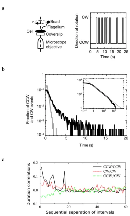
In 2004, single-cell experiments were performed by Korobkova et al. [38] on RP437, a widely used wild type (WT) strain of E. coli cells. They were able to attach a small bead (0.5µm) to one flagellum of a bacterium tethered to a surface and study the sequence of CW (tum-bles) and CCW (runs) events performed by the bead during 170 min-utes. (See diagram on Fig.3(a)).

From the analysis of the sequence they obtain a power law distri-bution for the times of run, instead of the exponential distridistri-bution expected from the work of Berg and Brown [7]. This can be seen in Fig. 3 (b). The tumble times stay exponentially distributed. The run and tumble times are temporally correlated (panel (c)) and the tumble biasing changes along the experiment. The corresponding time series of the binary switching pattern CCW  CW appears to show a power spectrum with 1/f-type behavior at low frequency [76]. It is unclear,

a b c 0 20 40 60 -0.1 0.0 0.1 0.2 CCW/CCW CW/CW

Sequential separation of intervals CCW/CW

Duration

cor

relations

Figure 3: Single motor statistics. (a) Schematic view of the experiment and binary time series indicating the direction of rotation. (b) Distri-bution of CW (tumbles, grey) and CCW (runs, black) intervals from a cell. Inset, cumulative distribution of the same CCW in-tervals (black line), corresponding to a power law with an expo-nent approximately −1.2 (gray straight line). From Korobkova et al. [38]. (c) Duration correlation and autocorrelation of CCW and

CW events. Figure from Tu and Grinstein [76] using the

however, if all the bacteria have the same power law exponent or if the exponent was part of a distribution.

The original idea of Khan and Macnab [37] about an energy bar-rier description for the CCW  CW transitions have been considered by Tu and Grinstein [76]. They have shown that white noise coming from the intrinsic stochastic nature of the signaling pathway kinetics and the reduced number of molecules inside the cell lead to a power-law regime in the CCW times distribution. Correlations between the duration times of nearby CCW (CW) intervals arise from the slow temporal dynamics of the mean CheYp level. Some other more so-phisticated models involving various molecular species composing the chemotactic pathway also predict power law CCW distributions due to low molecule numbers fluctuations [51].

In 2006 Wu et al. [79] have developed a method for three-dimensional tracking of bacteria from the unfocused images of bacteria. An anal-ysis of the accessed trajectories revealed a crossover to diffusion for times as large as 3.6 seconds, a value larger the standard Berg’s mea-surement (∼ 1s).

Based on the works by Korobkova et al. and Wu et al. some authors have predicted the existence of Lévy walks-type individual bacterial trajectories. However, there is no experimental confirmation of this or other consequences of the power law run time distribution.

Lévy walks in bacterial trajectories have recently be found by Ariel et al. [2], but for swarming bacteria. The mechanism underlying this superdiffusive behavior is fundamentally different than those hypoth-esized for swimming bacteria. Swarming bacteria do not behave like Lévy walker as a result of their run-and-tumble dynamics. Instead, it is the collective flow that induces the motion.

1.2.3 Swimming at low Reynolds numbers

Microorganisms move autonomously, free from any external force or torque in relatively viscous environments. The typical Reynolds num-ber for bacteria like E. coli is around 10−4 and essentially Stokes’ hy-drodynamics equation applies. Therefore, far from the swimmer, the velocity field can be model in leading approximation as a force dipole [41]. Then, two classes of swimmers can be distinguished: the “push-ers”, with the motor on the back as in the case of bacteria or sperm cells; and the “pullers” with the propulsive mechanism in the front, swimming with a breaststroke as algae. The corresponding velocity fields are shown in Fig. 4.

The velocity fields of pushers and pullers look similar, but with an inversion of velocity directions. This causes significant differences in their interactions with surfaces and other swimmers, and also the constitutive relations for the suspension [45].

a b

Figure 4: Velocity fields of (a) Echerichia coli and (b) Chlamydomonas rein-hardtii (from Drescher et al. [20] and [21]).

The presence of walls modifies the velocity field and bacteria are known to be attracted by flat surfaces. Several studies have shown that the concentration of bacteria is significantly larger at the top and bottom walls of square microchannels compared to the concentration in the bulk [8,20,28].

Bacteria described as pushers [20] are attracted to their specular hydrodynamic image close to a solid wall [8,14,18,42]. Furthermore, near a surface the rate of tumble has been observed to decrease with respect to the bulk [56], also contributing to the long time bacteria spend very close to solid surfaces [20,66]. On the other hand, a purely kinetic approach [25,43], not taking hydrodynamic interactions with walls into account, also predicts increased bacteria concentrations at walls in confined geometries.

Bacteria motion at the surface is also modified compared to motion in the bulk due to lubrication forces between swimmers and walls. The viscous drag acting on bacteria slows them down [18] and leads to the existence of circular trajectories due to their body rotation [4, 28, 40] . Moreover, the orientation (clockwise or counterclockwise) depends on surface properties [32].

1.2.4 Swimming in sheared flows

1.2.4.1 Bulk

In a shear flow, solid objects undergo periodic rotations known as Jeffery orbits [33]. A sphere rotates with constant angular velocity, whereas for an elongated body, such as a helix, the velocity depends on the orientation. The more elongated a body, the longer its resi-dence time when aligned with streamlines.

In addition, as underlined by Zöttl and Stark [82], in confined flows displaying a shear-gradient such as Poiseuille flows, families of quasi-periodic trajectories appear as a result of the shear gradient experi-enced by the swimmers. This result indicates that the transport and

dispersion properties of active suspensions are in this case non-trivial. This is currently a very open problem which outcome turns out to be qualitatively different from the standard hydrodynamic transport of passive colloidal particles [25].

Marcos et al. [48] have recently seen that bacteria drift perpendicu-lar to the shear plane in Poiseuille flows. The drift has been explained as a consequence of the interaction between the swimming bacterium (composed of chiral flagella attached to a body) and the shear flow [47,48]. As a consequence bacteria drift in opposite directions in the upper and lower half of a Poiseuille flow, induced by the opposite signs of the shear rate component.

The origin of chirality-dependent drift at low Reynolds number can be simply understood for the case of a helix. Consider the following example from Marcos et al. [47] of a right-handed helix aligned with a simple shear flow (Fig.5), and decompose the velocity at a segment of the helix into components perpendicular and parallel to the segment. The red and black solid lines in the inset represent the top and bottom halves of the helix. Drag on a thin rod in low Reynolds number flow is anisotropic, with a greater resistance when oriented perpendicular rather than parallel to the flow [13]. The perpendicular components of drag will add to produce a drift in the − ˆy direction. Changing the sign of the shear or reversing the chirality of the helix will result in a drift in the opposite direction. Furthermore, the drift depends on the orientation of the helix.

a b c

Vorticity direction

x y

Figure 5: (a) Sketch of a left-handed helix in simple shear flow. (b) Top view. The inset shows the net force acting on one pitch of the helix is along − ˆy (adapted from Marcos et al. [47]). (c) Sketch indicating

forces and torques acting on a bacterium in a shear flow (adapted from Marcos et al. [48]).

In addition to rotating in a Jeffery orbit, a helix drifts across stream-lines. The combination of a helix and a body attached to it in a shear flow results in a different phenomenology, as it has been explained by Marcos et al. [48]. A helix is subjected to a net chirality-induced

lateral force pulling it to the − ˆy direction, while the body will have a big hydrodynamic drag opposing the helix drift. The result is a torque aligning the bacterium to head the ˆy direction, which is the vorticity direction (see Fig. 5 (c)). Since the object is self-propelled, it will mi-grate in the vorticity direction. This phenomenon is purely physical, not as the case of fish and aquatic invertebrates’ rheotaxis, that are able to sense the shear and behaviorally respond to it [3,57,61].

1.2.4.2 Surfaces

Recent studies suggest that when swimming in the vicinity of a sur-face, upstream swimming takes place above a given threshold in shear rate for any front-back asymmetric microswimmer [77]. In the presence of the flow (but no cell propulsion), the swimmer’s head and flagellum are carried downstream by the flow, but the head expe-riences a larger resistive force, due to the hydrodynamic interaction with the wall, than does the flagellum. This larger resistance leads to a torque orienting the cell upstream. This mechanism is independent of flagella chirality and below a given threshold of fluid velocity, the swimmers can overcome the flow and migrate upstream [36], which is named “positive rheotaxis”.

Upstream swimming have been reported for mammalian sperm by Bretherton and Rothschild [9], Miki et al. [53] and Kanstler et al. [35], and for E. coli bacteria by Kaya and Koser [36] and our group [27]. However, while rheotaxis has been observed for bacteria navigation in the bulk of a flow (i.e., far from surfaces and edges) [48], there is no report of continuous upstream motion in such environment.

In addition, the coupling with the chirality-induced torque on bac-teria result in a diagonal orientation of the swimmer, with a compo-nent facing upstream and a transversal compocompo-nent facing the local vorticity direction. This angle against the flow is function of the ap-plied shear rate and at high shear rates bacteria orient perpendicular to the flow direction. Although this is qualitatively understood, to our knowledge there is not yet a model explaining the angular distri-bution of bacteria orientation under flow close to surfaces.

The combination of bacteria swimming at a given angle and bac-teria transport by the flow leads to diagonal trajectories in the flow. Since the transversal orientation depends on the vorticity direction, bacteria trajectories are thus oriented in opposite directions at top and bottom surfaces of a microchannel.

Concentration profiles stay flat in the bulk with a strong increase of concentration at the surfaces for small applied shear rates [29], but for higher shear rates more complex concentration profiles have been observed and predicted in the direction of the channel height [14,25, 62]. Ezhilan and Saintillan [25] and Chilukuri, Collins, and Underhill [14] predict a decrease of the surface concentration with increasing shear rate, but to our knowledge no experimental investigation of

this phenomenon, previous than ours [27], has been performed so far.

Less work has been devoted to the study of bacteria motion at wall interceptions. Bacteria concentration have been found to be even higher at these edges compared to flat surfaces [1] and under flow bacteria motion at the edges is observed in a predominantly upstream way [1,30] over long distances. This upstream motion is at the origin of anomalous reconcentrations observed to be closely linked to the specific details of the confining structure [1,26].

The rich phenomenology exposed up to here is nothing but a small part of the known bacterial behavior in diluted suspensions. It is, how-ever, almost the minimal knowledge necessary for the understanding of the rest of this work and the results that will be presented.

1.3 o r g a n i z at i o n

In the rest of the thesis we will focus first, on the development of a Lagrangian tracking technique for accessing the three spatial coor-dinates of bacterial trajectories. Using this tool we study some fea-tures of individual bacterial behavior in the bulk of Newtonian and non-Newtonian fluids, as well as in more concentrated active suspen-sions. Later, we study the properties of the bacterial transport under flow close to the surfaces and edges of confined channels. Finally, we tackle the practical case of upstream bacterial contamination in very confined structures.

A synthesis of every chapter is exposed below.

Chapter2 3d lagrangian tracker – We present a technique of Lagrangian 3D tracking of fluorescent microscopic objects. It provides the 3D object trajectory and a direct image of the particle in its close environment. We test its performance by tracking fluorescent beads undergoing Brownian motion, as well as under flow.

Chapter3 three-dimensional motion of bacteria – Using the developed instrument from the previous chapter, we study the three-dimensional trajectories of E. coli bacteria in motion and find a different behavior from the globally accepted run-and-tumble picture with exponentially distributed run and tumble times. We find a great diversity between bacteria from the same bath, which manifests as variability in the magnitude and fluctuations of velocity and persis-tence of trajectories. This is in agreement with the scientific literature regarding individual cell’s behavior in tethered conditions.

We measure the rotational diffusion coefficient from 3D tracks and report values that are widely dispersed. We compare the results for various strains of run-and-tumble bacteria and a strain of smooth swimmers. This large distribution is found to be robust to changes in concentration, to chemical environment and also to changes of E. coli

strains. We relate the large distribution of orientation persistence to the motor rotation statistics.

We track bacteria in polymeric suspensions, presenting shear thin-ning and viscoelasticity. We find a rectification of the trajectories for the higher polymer concentrations, that we are able to explain only considering the shear thinning effects.

From the tracking of fluorescent cells in a more crowded suspen-sion of non-fluorescent bacteria, we have identified a dependence between the bacterium’s activity and the exponent displayed by its superdiffusive behavior.

Chapter4 transfer and traffic in a confined flow – We quantitatively study the transport of E. coli near the walls of confined microfluidic channels, and in more detail along the edges formed by the interception of two perpendicular walls. Our experiments estab-lish the connection between bacteria motion at the flat surface and at the edges and demonstrate the robustness of the upstream motion at the edges. Upstream migration of E. coli at the edges is possible at much larger flow rates compared to motion at the flat surfaces. Interestingly, the bacteria speed at the edges mainly results from col-lisions between bacteria moving along this single line. We show that upstream motion not only takes place at the edge but also in an “edge boundary layer” whose size varies with the applied flow rate. We quantify the bacteria fluxes along the bottom walls and the edges and show that they result from both the transport velocity of bacteria and the decrease of surface concentration with increasing flow rate due to erosion processes. We rationalize our findings as a function of the local variations of the shear rate in the rectangular channels and hydrodynamic attractive forces between bacteria and walls.

Chapter5 upstream contamination in narrow channels – At the end we study the upstream migration of bacteria in extremely confined environments. This comprises swimming in the bulk and on the surfaces and edges of the confining structures. We demonstrate the possibility of a net transport of bacteria established against the flow for specific flow and confinement conditions. We study the up-stream invasion of bacteria from a reservoir towards a source of clean liquid as a function of the bacterial velocity and imposed perfusion flow. We have found that the persistence in individual trajectories, previously identified in chapter3, is at the origin of supercontamina-tion processes, therefore, influencing the macroscopic transport prop-erties. We explain quantitatively our observations based on a simple model, which makes the link between the motor statistics and the macroscopic transport of bacteria.

2

3D L A G R A N G I A N T R A C K E R

In a 1972 seminal work, Berg and Brown have shown that tracking individual micro-organisms in 3D was a determinant step to under-stand bacterial motility and chemotactic response to chemical gradi-ents [7]. At that time the device built by Berg and suited to perform the tracking and 3D trajectory reconstruction, was conceptually and technically outstanding [5].

Since then, other techniques of 3D tracking have emerged For exam-ple, the development of fast piezo scanning has allowed high speed image stack acquisition techniques. This was used to reconstruct by post analysis micro-organisms swimming trajectories [15]. This method though very potent to obtain multiple object trajectories finds its lim-itation, if the object speed is high. Also, it turns out to be strongly de-pendent on free computer memory capacities limiting the long time tracking possibilities. Interestingly, there are alternative techniques using the defocussing rings of fluorescent particles to access the XYZ position and a large number of tracks at the same time [79]. The lim-itation here is the complexity of the post-analysis, increasing with the particle concentration and also the limited range in Z exploration. Past the year 2000, there was a surge in the development of holo-graphic 3D particle reconstruction techniques (see for example a re-view by Memmolo et al. [52] and refs inside). This tracking method allows by post-analysis, the 3D reconstruction of few simple objects trajectories such as the Brownian motion of spherical colloids [11] and bacteria [63]. This method has led recently to important advances in the understanding of sperm swimming trajectories [34,73].

However, these recent 3D tracking methods are of Eulerian type, meaning that the volume of observation is fixed in the laboratory ref-erence frame. It is important to notice that inherently, such Eulerian methods may lead to a systematic statistical bias as, for trajectories displaying large persistent speed, the particles are likely to leave the volume of observation faster than for other trajectories undergoing for example, a diffusive motion.

Lately, increasing interest into the swimming dynamics of micro-organisms made the development of reliable Lagrangian tracking techniques using modern tools [44] particularly important again. Here we present a technique of Lagrangian 3D tracking extending the work of Berg with modern tools of visualization which allow for a time resolved refocusing of a fluorescent object (Fig. 6). The fluorescent particle can be studied in a quiescent fluid as well as in an imposed flow. It has the advantage of providing, besides the full 3D object

jectory, a direct image of the particle in its close environment. The same system can also be used to track fluorescent passive objects like silica or latex tracers, to be used, for example, for an accurate deter-mination of the flow velocity profiles in microfluidic devices (Fig.16). In addition, a unique feature of this technique is the possibility to track only the bright spots in a crowded environment of opaque ob-jects, such as specific fluorescent bacteria in a suspension of normal bacteria displaying collective motion.

Microfluidic chamber XY mechanical stage Camera Objective lens I/O Labview program Z piezo stage Z X Y Trapping area X Y

Figure 6: Experimental set-up. The tracking systems consists of two super-posed stages mounted on an inverted microscope. The horizon-tal xy position is controlled mechanically and the z-position via a piezoelectric positioner. The targeted fluorescent particle position is visualized in a given so-called “trapping area” by a CCD cam-era. The image is transferred to a Labview program processing the information. The program assesses the current xy and z positions and commands the mechanical and the piezo stages to move to a new position such as to keep the particle in focus and close to the trap center. The outputs are the xyz position and a video of the particle surrounding.

2.1 e x p e r i m e n ta l s e t-up

The set-up is sketched in Fig.6. It is composed of an inverted micro-scope (Zeiss-Observer, Z1) with a high magnification objective (100 × /0.9DIC Zeiss EC Epiplan-Neofluar), an xy mechanically controllable stage with a z piezo-mover from ASI and a digital camera ANDOR iXon 897 EMCCD. The camera output and the stage input/output signals are connected to a multi-threaded Labview software capable of reassigning, by a real-time feedback loop, the stage position and to keep one particle in focus in the central visualization field region (see Fig. 6). The ANDOR camera is very sensitive (pixel size 16 microns)

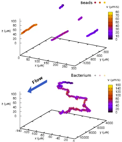
Figure 7: 3D track of latex beads (top) and a bacterium (bottom) under flow in the same experiment. The color code stands for local velocities in micrometers per second. The michochannel spans from z = 0µm to 110µm in height, and the width from x = −300µm to x = 300µm. The length is approximately 150mm. The bacterium here is a wild-type strain of E. coli (RP 437), transfected with a Yellow fluorescent plasmid.

and suited to visualize weak fluorescent signals. It is thus relatively slow, working nominally at 30 fps on a 512 × 512 pix2 matrix. Here, we present the performances achieved at a faster tracking speed of 80Hzreducing the spatial resolution to 128 × 128 pix2. The tracking limitations come essentially from the z exploration limits. The z-piezo module used here, has a range of exploration of 500µm, however in the present case, the vertical exploration limitation stems essentially from the 100× objective working distance which is of 150µm.

From the coordinates of the stage in the laboratory reference frame and the position of the target object in the images, we obtain the three-dimensional trajectories and also a video recording of the fluorescent targeted object. In Fig.16, we present some tracking results obtained with this technique, for passive tracers and for a bacterium in a Hele-Shaw microfluidic cell under flow.

Note that the same technique can also be adapted to an objective of lesser magnification or to a much faster (though less sensitive) SC-MOS technology. The rate of transfer of visual information, its pro-cessing and the reaction of the mechanical and piezo-components of the XY and Z stages have in all cases to be adapted to the current ma-terial possibilities. Nevertheless, the method described here remains valid despite possible changes of visualization technology.

2.1.1 General algorithm

In the following, we detail the general detection algorithm. First, when a fluorescent particle reaches the trapping area, the user can decide by clicking on the mouse to start the tracking process. The first action of the detector is to determine the XY position of the targeted object, put it in the center by moving the XY mechanical stage. Then the system proceeds by scanning very rapidly in Z to get a defocussing refocus-ing video that will immediately be analyzed. This first step allows to determine several initialization parameters that will be used subse-quently to specify the detection functions. Then, the algorithm starts to work in the nominal mode. At every iteration step of the detection algorithm, an image (Image(t)) is obtained as well as the current stage coordinates and transferred to the labview program. The target position in the image reference frame, is determined and a move is performed by the stages before the next image exposure in t + dt, in order to keep the object in focus. For each iteration the determined object position and the image are recorded. In the following , we de-tail the principles of XY and of Z detection and thereafter, the XY and Z stage motions. Finally, we address the question of tracking perfor-mances.

2.1.1.1 XY detection

To track the targeted object in two-dimensions, we use a standard im-age processing method. The object xyC coordinates in the microflu-idic chamber reference frame, are composed of the xyS coordinates of the stage in the laboratory reference frame when the image was exposed, and the xyI coordinates of the object in the image:

xy_C(t) = xy_I(t) − xy_S(t). (4)

Note that the object does not need to be in the center of the image to determine its xylposition, keeping it in the image bound is enough. To determine xyC(t + dt), knowing xyI(t) and xyS(t + dt), we de-fine in Image(t + dt) a search area (extracted Region Of Interest, ROI) around the position xyI(t)where the object is expected to be in the new image. This ROI is pre-processed (Gaussian filter and lo-cal threshold) to get a binary image with background correction and

to obtain a set of binarized objects. The objects are filtered to keep the ones of a predefined size and the positions of their geometrical centers are determined. We keep as xyC(t + dt) the closest object to the former position xyC(t). Note that we could easily introduce some memory (as we did for z) to handle for example, a collisional interac-tion of two similar particles such as to decipher the trajectory continu-ity of both objects. Also, for the object detection other methods could be used, like the maximum correlation with a mask. However, the present one turns out to be quite efficient yielding a computational time under 5ms, which allows a margin of 5ms for the z computing and the stage motion, compatible -in principle- with a tracking at 100 frames per second.

2.1.1.2 Z detection

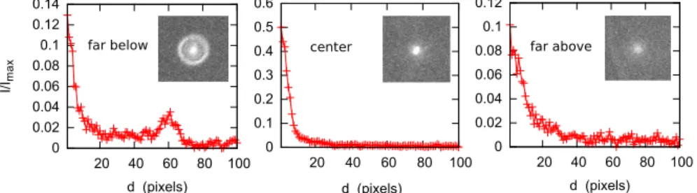
The principle for the z detection differs significantly from the hori-zontal xy coordinates assessment. It is based on an optimized search for a vertical position suited to keep the moving object in focus. The algorithm keeps the object in focus by minimizing the apparent ob-ject width w. The obob-ject width is minimal when it is in focus and grows as it is far from the focal plane both above or below as shown in Fig. 9. We could also have used the maximum of light intensity as a determinant for the focus value, but the width minimum allows us to account for the photo-bleaching of the target and it turns out to be a more robust criterion, since it is less sensitive to the noise induced by the presence of other bright objects that may temporally appear in the background. 0 0.1 0.2 0.3 0.4 0.5 0.6 20 40 60 80 100 0 0.02 0.04 0.06 0.08 0.1 0.12 20 40 60 80 100 d (pixels) far below center far above

0 0.02 0.04 0.06 0.08 0.1 0.12 0.14 20 40 60 80 100 I/Im a x d (pixels) d (pixels)

Figure 8: Normalized intensity profile as a function of the distance d to the

center of the particle. Imax is the absolute intensity maximum

when the particle is in focus.

Once the xy object position on the image has been determined, the mean radial profile around xyI(t)is computed , i.e. the average inten-sity (I) as a function of the distance to the center (d). As a convention, we compute the width of the object (w) as twice the distance to the center at which the intensity has dropped to one half of the central maximum. Fig.8shows the radial intensity profile for three positions of the focal plane, below, close and above the particle.

0 2 4 6 8 10 12 14 -10 -5 0 5 10 w/2 (pixels) Δz µm) w₊/2 =1.5+0.4*z+0.02z2 w-/2 =1.8-0.4*z+0.11z2 ( far below far above center

Figure 9: Half width of the particle as a function of the distance between object and focal plane. The particle is in focus at ∆z = 0.

All along the tracking process, the minimum detected width wmin and the central intensity Imaxat the moment of the minimum width detection, are kept in memory. Whenever a smaller width is encoun-tered through the tracking process, its value becomes the new wmin and the maximum intensity replaces the Imax. The regular update of these parameters allow to keep track of the photo-bleaching that produces a drastic intensity decrease and a reduction in the object ap-parent size on the long run. The initial values of wmin and Imax are set at the beginning of the track by a procedure that we will described later.

The vertical coordinate zC of the object is defined as the sum of the coordinate of the stage zS in the laboratory reference, plus a cor-rection ∆z representing its distance to the focal plane. In this way, z_C = z_S− ∆zwhere ∆z can be positive or negative and is zero when the object is in focus (see Fig. 9). For the computation of ∆z we de-fined several criteria depending on the image of the object. The fea-tures of this function, allow to define three main possible regions for the position of the focal plane zS: (i) The far region below the object, when the focal plane is below the object (∆z < 0) , (ii) the far region above the object, when the focal plane is far above (∆z > 0) and (iii) the close central region as depicted in Fig.10.

Far below - The far region below the object (z position above the focal plane) is characterized by the presence of rings around the parti-cle (Fig.10). Typically, the rings appear when the object is more than 6µmabove the focal plane position. By measuring the radius R of the first ring one can estimate ∆z. The ring size as a function of the dis-tance to the object is approximately linear up to 20µm from the object. This relation allows the reaching of the close central region out of a calibration which is particle and system dependent. Then ∆z = cR.

Far above - In the far region above the object, the particle appears as a wide and fuzzy white dot of low intensity with no ring. If the maximum object intensity I(t) is lower than a given fraction of the

cur-objective

Δ

z

z

z

z

Figure 10: Sketch illustrating the regions of detection for an E.coli fluores-cent bacterium : the bacterium position and possible stage posi-tion.

rently stored Imaxvalue (this coefficient is typically set to 0.4 but can be adjusted), the algorithm recognizes that the focal plane is in the far region above the object. We have a calibrated function for the width of the particle as a function of its distance to the focus value w+(z). The correction will be calculated as ∆z(w, wmin) = (w − wmin) _dwdz₊

w.

It is a second order polynomial represented in Fig.9by the solid line on the right side of the curve.

The detection of this region takes place closer to the object than in the former case of the rings, this implies that a descending bac-terium is better followed, i.e. with less noise, than a bacbac-terium with an increasing z coordinate.

Central region - When the focal plane is in the central region of Fig. 10, from the scanning of a fixed “standard” fluorescent object (here a bacterium), two piece-wise curves for the object’s width were fitted as a function to the distance to its center (Fig. 9). One curve for ∆z < 0 (w−(|∆z|), below the object) and the other one for ∆z > 0 (w+(|∆z|), above the object). The center ∆z = 0 is a local minimum and close enough to it, the two curves are almost symmetric.

From the image, one cannot know whether the focal plane is slightly above or below the object, therefore we have chosen the right branch w₊(|∆z|) that works reasonably good in both cases. We relate the ob-ject’s position to the measured width w by means of the inverse func-tion. The absolute value will be|∆z|(w, wmin) = (w − wmin) _dwdz

 _w.

and the sign depends on whether the last stage move was suc-cessful (corresponding to width decrease) or not (corresponding to a width increase). If the last step was successful, we keep its direction and if not we invert it. As a result, the stage fluctuates around the zC object position. Start detec�on Compute Mean radial profile Ring detect Object Image Radial profile Yes No detected No Yes Compute d Below Above Center Δ z=c R Δ z = (w−wmin) ∂z ∂ w

|

|

Figure 11: Flow diagram of the z detection indicating in details the proce-dure for the coordinate determination starting from the object image. R = 0 means that no ring was detected.

2.1.1.3 XYand Z stage displacement

During the tracking initiation procedure, the fast z-scan yields a se-quence of images typically separated 0.5µm around the object. For every image, the object width (w) is determined and thereafter the minimum width wmin. From the image giving wmin we also get and store the maximum intensity Imax and position zC. At the end of this sweep, the stages goes to the best z coordinate and the tracking variables are fully initialized.

For the xy stage motion, a proportional integrative derivative (PID) algorithm is used and empirically tuned, to perform a progressive motion. This avoids to couple directly the detection and displace-ment, that would keep the object strictly centered in the image and which may introduce spurious mechanical perturbations and

instabil-ities due to abrupt movements. This is possible since for xy detection we just need to keep the object in trapping zone and determined the true position from the particle center analysis.

For the z stage displacement, when the detected region is far below or above, the stage is moved with a value ∆zS(w, wmin) = ∆z(w, wmin) and reaches the central region in one step.

In the central region, the stage is moved at a displacement mag-nitude ∆zS(w, wmin,~vz) where we take into account a second or-der contribution to the position, incorporating in the computation the object displacement between two consecutive images. This way, ∆z_S(w, wmin, vz) = ∆z(w, wmin) − k(w, wmin)vz∆t, where vz is the object velocity along z, computed in real time from the previous dis-placement. The coefficient k(w, wmin) is positive between 0 and 1, being 0 when w is close to wmin and 1 for low values of the ratio wmin/w. We use the empirical extrapolation function k(w, wmin) =

1 2 h tanh(0.95−wmin/w 0.05 ) + 1 i .

As said previously, the sign of ∆z(w) depends on the improvement (minimization) of w when compared to the previous step. Due to the buffer of the camera, we obtain the images with a delay of two periods of sampling, then, the more recent captured image is not a direct consequence of the last order given to the stage. To avoid taking bad decisions due to this lack of synchronization we have lowered the frequency of sampling and actuating in z to one third of the one in xy.

Importantly, the xy motion is performed using two lead screws, one for each axis. An inherent feature of such mechanical displacement stage is the existence of a backlash, i.e. the screws need some finite back-rotation to restart a reverse motion. For our system the backlash is of the order of 1µm. Since our stage controller uses rotary encoders, this repetitive error is not visible from the recorded stage data. So, we use a correction algorithm in the post-processing to remove this error from the track data. An improvement for the setup would be to replace the rotary encoder with an optical linear encoder which returns the real position of the stage, thus processing the backlash in real time.

2.1.1.4 Backlash correction

Now we describe how to correct the mechanical backlash inherent to mechanical systems as soon as there is an amount of clearance between mated mechanical components, like gear teeth. The backlash manifests itself when the motion direction is reversed and the slack or lost motion is taken up before the reversal of motion is completed. In the case of our tracking microscope, the mechanism for the xy displacement is mechanical, therefore, not exempt of backlash. The zdisplacement is a piezoelectric displacement, allowing essentially a high precision positioning at the nanometer scale.

In general, for many high precision microscopic devices, the stages allow to perform very precise displacements by following an algo-rithm for motion allowing to work around the backlash. Before a move, the stage goes to an intermediate position far away allowing to always come from the same direction to the targeted position. This is certainly not suitable for bacteria tracking, where the stages have to “follow” the swimmer as it moves. Here we compensate for the stage backlash in a post-processing treatment of the trajectories. Note that this step is crucial and special care needs to be taken when building a 3D tracking device to avoid false data recording due to backlash problems.

The first step is to characterize the backlash magnitude along the x and y directions. To this purpose, we tracked a fluorescent latex bead stuck on a glass plate, switching off the moving capability of the stage. In this condition, the software recognizes the particle po-sition but does not move the stage to have it in focus. We start the tracking with the bead in focus in the center of the image and man-ually displace the stage in xy by means of the joystick while always keeping the particle in the image. In this case the bead displacement in the image should be equal to the stage displacement, and the sum should compensate at every time since the particle did not move with respect to the microfluidic chamber (see equation (4)). The apparent displacements with respect to the chamber are due to the backlash error. Fig.12shows with black circles in the top the y_S stage position as we move it, and using the same scale in the bottom the resultant position of the object yC in the chamber is shown. We can then see that the later is not of constant value, but it is shifted by an quasi con-stant value of 2µm every time the direction of the stage is reversed and the stage displaces more than this distance.

To compensate for the backlash, we have analyzed independently the xS and yS stage coordinates’ response to a motion reversal. As the stage moves and changes direction along one or both x or y, xS or yS will inverse displacement direction and the indicated stage po-sition will be false. The stage may still be in the same place until the backlash is overcome. As a consequence, a wrong displacement information is introduced in the stage coordinates. To correct for the stage position, we assume that a real displacement does not take place until it is bigger than a certain distance dx in the case of motion in-version along x (or dy for backward motion along y). Once this gap is overcome, the rest of the trajectory is shifted to match the previous position where the stage was clutched. This correction can be seen in Fig. 12(top). It results in a delay every time the direction is inverted with a subsequent reduction of stage displacement. The final particle position in the channel is affected following equation (4). We repeat this procedure for different values of dx and dy independently and determine the values dx∗ and dy∗that minimize the standard

424 426 428 430 432 434 436 438 440 yS ( µ m) raw corrected 430 432 434 2495 2500 2505 2510 2515 2520 yC ( µ m) Frames

Figure 12: y coordinates of the stage (top) and particle position (bottom). Black circles are the raw measurements and the red line the same magnitudes after backlash correction.

tion of the corrected positions xC and yC. These turn the step func-tion in Fig. 12 (bottom) into an almost constant red line that better reflects the fixed position with respect to the chamber. The optimal values dx∗ = 0.45µm and dy∗ = 2.0µm turn out to be the same for independent realizations of the stage displacements.

2.1.2 Assessment of tracking performances

To assess the quality of the tracking method we follow latex beads performing Brownian motion. Due to the intrinsic difference in the tracking principles in XY and Z we separate the analysis. The motion in X and Y stemming from an endless screw machinery, the main source of uncertainty comes from the presence of backlash. Random Brownian motion is indeed a severe test. On the other hand, the main source of uncertainty for the Z position is not the backlash (piezo device), but the quality of the Z detection algorithm. Note that for the present fluorescent objects the Z detection algorithm is not a zero-crossing but a minimum detection method much less accurate to fix precisely a position.

For the X and Y coordinates, we first followed a diffusive latex bead in a quiescent suspension by switching off the moving capability of the stage. The position of the particle is determined in real time solely by the image analysis part of the algorithm, as long as the particle remains in the region of visualization. The hence obtained trajectories are typical of a thermal Brownian of diffusion coefficient D_E = kBT

6πµa according to Einstein’s relation, where a is the particle radius and µ the fluid viscosity. For the particle of Fig. 13 (a) which

is a round latex particle of diameter 1.75µm from Beckman Coulter (std = 0.02µm), the theoretical diffusion coefficient in water at 26oC would be DE = 0.29µm2/s. Its mean squared displacement (MSD) is defined as(~r(t + ∆t) −~r(t))2

t = 4D∆tin two dimensions, where the brackets denote the average along the time length of the trajectory. From the slope of the MSD we extract the diffusion coefficient D = 0.3215 ± 0.0004µm2_{/s. See thick line in Fig.13(b).}

a b -2 0 2 4 x ( µm) -1 0 1 2 3 4 5 y ( µ m) 0 2 4 6 time lag ∆ t (s) 0 2 4 6 8 10 12 MSD ( µ m 2 ) fixed stage moving stage corrected backlash

Figure 13: Tracking of Brownian particles. (a) 2D trajectory of Brownian mo-tion of a latex bead obtained with no moving stage. Depicted length 20s starting from (0,0) coordinates. The beginning and end of the trajectory segment are marked with red spots. (b) Mean squared displacement for a trajectory of the same bead obtained with no moving stage (solid thick line), and for a moving stage with no backlash correction (thin solid line) and same track after backlash correction (thick dashed line).

To avoid the lack of statistics affecting the measurement for this cal-culation we have only considered time lags smaller than one-tenth of the track length. Nevertheless, the MSD of the different components X and Y have different slopes for different realizations, where the difference can be as large as 15 percent. This asymmetry evidences the shortness of the trajectory. The differences between the theoreti-cal and experimental diffusion coefficient found can also arise from the uncertainty in the absolute determination of the colloid radius.

Now we track the same particle as before, but with a moving stage. The tracking procedure will keep the particle in the trapping area (see Fig.6). In this case, the obtained trajectory is affected by all the issues associated with the mechanical response of the stage. The signature of an uncorrected backlash in a Brownian object tracking is an offset and oscillations in the mean squared displacement plot as in Fig. 13 (a) (thin black solid line). When the obtained trajectory is corrected with the above explained method, using the found values of dx∗ and dy∗ independently for each horizontal axis, the MSD curve becomes a straight line (thin red dashed line) and the diffusion coefficient

mea-sured from this corrected track is 0.3085 ± 0.0005µm2_{/s. This value is} 96 percent close to the previously determined for a fixed stage, the difference is in the margin of the previously found asymmetry in the individual components.

Now we address the question of the Z component.

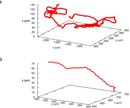
We performed a 3D tracking of a bead undergoing slow sedimen-tation (carboxylate particle from Polysciences of diameter 1.62µm, std = 1.65µm, ρ = 1.05g/cm3) that we represent in Fig. 14 (a). The sedimentation speed is about 0.02µm/s which is close to the theo-retically expected value. The diffusion coefficients for each of the three spacial directions agree withing 10 percent. The global diffu-sion coefficient keeps within the error margin of the expected value D_E = 0.311µm2_{/s. We have experimentally found D = 0.309µm}2_/s. The MSD versus time lag for the three directions, after backlash cor-rection in x and y, are represented in Fig. 14 (b). From this test we conclude that the Z tracking method is reliable for this kind of prob-lems. a b -5 -10 -8 -6 -4 -2 z ( µ m) 0 -10 2 x ( µm) 0 y ( µm) -5 5 0 0 5 10 15 time lag "t(s) 0 2 4 6 8 10 MSD ( 7 m 2 ) Theory X Y Z

Figure 14: Tracking of a Brownian particle during sedimentation. (a) 3D tra-jectory corresponding to 31s. (b) MSD by components. The X and

Y components have had backlash correction. We have subtracted

the drift velocity and found agreement between the three spatial coordinates.

Note that tracking Brownian particles is the most difficult situation for a stage in terms of backlash. The tracking of swimmers or objects under flow will introduce this error much less often, since their tra-jectories will be more persistent. As our method of correcting for the backlash works well for Brownian motion we are thus confident that is correctly treats swimming bacteria or objects transported under flow.

The captured trajectories contain the mark of the backlash as well as additional noise introduced by the tracking device. This noise can occur at various stages of the tracking process: in the detection phase when applying a local threshold to the image, during the stage

mo-tion due to the mechanical response of the stage or due to temporal delays concerning computer time and data transfer between the cam-era, the computer and the stage.

The uncertainties in x and y coordinates have different values in the case of one direction motion or when direction reverses often, since bigger uncertainties are introduced during the backlash correction. From the noise in detection of the fixed bead used for the backlash correction we determine standard deviations of 0.02µm when there is not backlash at play. The backlash correction introduces an extra uncertainty of 0.17µm.

For determining the uncertainties in z detection we analyze our bead during sedimentation in Fig. 14. The displacements between two consecutive images in x and y will be due to Brownian motion plus the horizontal backlash and noise in horizontal detection. These variations are normally distributed with standard deviation 0.09µm around zero. The displacements along z, after subtraction of the sed-imentation contribution, are due to Brownian motion plus detection uncertainties in z. These have a more flat distribution, also centered in zero with standard deviation 0.3µm. Since this latter distribution is wider than the expected one for Brownian motion comprised in the ones of x and y, we conclude that it is a consequence and a measure of the less precise position determination in z.

To address the time resolution of the device, the spectral response of the Brownian particle of diameter 1.62µm of Fig. 14 is shown on Fig. 15. We can see the 1/f2 decay expected for Brownian motion. The spectrum of y has a peak at around 1Hz. It was introduced by the backlash correction since the raw data do not present this feature. For the z coordinate, the noise increases starting from a few Hertz, and has a cut off at the effective sampling frequency 80/3 ≈ 26.7Hz which corresponds to the sampling frequency in Z.

The sampling frequency being 80Hz in X and Y and of 26.6 in Z, should allow us to track bacteria with resolution high enough to study the tumbling events (0.1s∼ 8 frames). We can even study peri-odic phenomena up to 40Hz in X and Y, like the wobbling dynamics of bacteria [44,58].

Moreover, we have also tested this device for tracking under flow and we have been able to follow bright objects moving at the high speeds of 160µm/s in XY and at around 40µm/s along the Z direction.

In the following chapter we will use the tracking device to study fundamental questions about the motility of bacteria in different phys-ical and chemphys-ical environments.

10-3 10-2 10-1 100 101 102 f (Hz) 10-10 10-5 100 105 Power Spectrum X Y slope -2 10-3 10-2 10-1 100 101 102 f (Hz) 10-10 10-5 100 105 Power Spectrum Z slope -2

3

T H R E E - D I M E N S I O N A L M O T I O N O F B A C T E R I A

Escherichia coli bacteria has become the paradigmatic example for the run-and-tumble particle realization. It has promoted the recent devel-opment of a statistical mechanics of active fluids of run-and-tumble particles [46,67] in parallel with active-Brownian particles [10].

Here we study the three-dimensional trajectories of E. coli bacte-ria in motion in different chemical and physical environments and at different concentrations. We find that the swimming dynamics is different from the globally accepted behavior described by Berg and Brown in their famous paper of 1972 [7].

3.1 e x p e r i m e n ta l s e t-up and methods

We study a drop of a very diluted suspension of bacteria, placed be-tween two microscope’s slides separated a distance H = 250µm. Ini-tially the concentration is extremely low, typically 105_bact/mL, corre-sponding to a volume fraction φ = 10−7_{. For computing the volume} fraction we have assumed the volume of the cells to be 1µm3. We use the same setup for experiments varying the viscosity and rheology conditions of the surrounding fluid.

The very diluted suspensions are used in all but one experiment, where we mix fluorescent and non-fluorescent bacteria up to a vol-ume fraction φ = 6 × 10−3_{. Otherwise, the great dilution guarantees} enough oxygen in the medium for very long times, even when the boundaries are not permeable to gases.

The system is put on the stage of our tracking microscope and the cells are tracked at 80 frames per second while swimming in the lower 150µm of the chamber. The chamber is closed on the sides, so the advective flows are limited and bacteria swim in no-flow condi-tions. As we will mainly be interested in studying the 3D swimming of bacteria, we have chosen a measurement chamber higher than the maximal Z-span distance of the tracking device. This way we maxi-mize the measurement length in the bulk.

Typically, bacteria describe circles on the bottom surface and even-tually take off to swim in the bulk, where they have a different dy-namics (Fig.16). We analyze independently the bulk and surface seg-ments of individual trajectories, defining by bulk the region 10µm farther from the solid surface.

Bacteria suspension – We use different strains of E. coli (RP437, AB1157, CR20) transfected with a fluorescent plasmid and prepared by the following protocol: 10µL of bacteria are grown overnight in 2.5

-710 -700 -690 -680 -670 -660 -650 -640 -450 -420 -390 -360 0 20 40 60 80 100 120 140 z (µm) x (µm) y (µm) z (µm) v (µm/s) 10 15 20 25 30 35 40 45 50

Figure 16: 3D trajectory of an E. coli RP437 bacterium. It starts describing circles on the bottom surface and later it abandons the bottom for the bulk. The color code represents the velocity in microns per second. Bulk part for 10µm < z < 150µm.

mL of the rich culture medium (M9G) plus antibiotics1

. This is placed in the incubator at 30°C and shaking at 250rpm until the culture reach optical density 0.5 for a wavelength of 595nm that we measure using an spectrophotometer. We have a calibration curve allowing the de-termination of the bacterial concentration by the measurement of the optical density of the suspension.

This culture is centrifuged, the supernatant removed and the pellet re-suspended in 2.5mL of water. After centrifugation the new super-natant is retired and the pellet is re-suspended into Motility Buffer, mixed with polyvinylpyrrolidone (PVP-360 kDa: 0.002%) and L-Serine (0.04g/mL). We will refer to this medium as MB+LS. After incubating for 30 minutes in MB+LS to obtain a maximal activity, a reduced num-ber of bacteria are transferred to the cell of measurements, containing the same solution that the reservoir but in which the swimmers will be in very low concentration. Other procedures, like re-suspending in Motility Buffer without L-Serine, in M9G medium, in polymeric solutions or in solutions with crowded non-fluorescent bacteria have also been used and whenever it will be the case it will be clarified through the text.

The three strains used are run-and-tumble cells in the case of RP437 and AB1157, and a strain of non tumbler mutants CR20 to which we refer as smooth swimmers , that almost never tumble. CR20 is a mu-tant strain derived from RP437 and it keeps most of its characteristics.

1 The antibiotics is used to impose a selection pressure on the culture. Bacteria carry in the same circular DNA sequence the gene for being resistant to the specific an-tibiotics and the gene to be fluorescent. The expression of fluoresce represents an energetic cost for bacteria and some of them manage to lose the fluoresce. At the same time they lose the resistance to antibiotics and die, resulting in a culture of only fluorescent bacteria.

3.1.1 Data processing

The data coming from the 3D tracker will be first subjected to back-lash correction in the x and y coordinates, as explained in 2.1.1.4.

It may happen, during the tracking process, that some image fail to be saved or that the tracker get “confused” and follow for a moment a different object and we decide to manually eliminate a few bad points from the trajectory. In these cases there will be holes in the track that we will fill with a linear interpolation, in the three spatial coordinates and the time, between the separated pieces of trajectory. This is cer-tainly not taking place very often and depends on how bright the bacteria are. The brighter the bacterium, the lower the probability to have this problem. It typically happens one or two times in a forty-minute set of tracks.

As the sampling frequency in z is one-third of the frame rate (see Chapter 2), the z values change only every three points. We filter these performing the average on a moving window over ten points, equivalent to 0.125s.

The next step is the correction of bad points in z. Sometimes dur-ing the trackdur-ing process for a window of points the detected values of z are very different to their neighbors. This may happen, for exam-ple, when another bacterium crosses the targeted-one and the signal is affected. We detect these points when their local velocity in z is unusually large, i.e. larger than twice the mean velocity for the tra-jectory. In this cases we replace the wrong z coordinates by a linear interpolation between the neighboring good points.

The samples that we put in the tracking device are, in general, not perfectly horizontal. In this case the xy plane of the microscope will not be absolutely parallel to the bottom of the microfluidic cell. Now we proceed to a rotation of coordinates to have the new xy coordi-nates parallel to the bottom. Later on we do a translation to have the zero in z coincide with the bottom of the cell.

At this point, the three coordinates are similarly treated. For de-termining the local velocity ~v and acceleration ~aof the swimmer we analyze independently x, y and z. For simplicity in the explanation let’s use x as example. To determine the local component the of veloc-ity vx(i)in the i − th position inside the trajectory, we get the sublist of coordinates around this point [x(i − n), . . . , x(i), . . . , x(i + n)] and perform a polynomial fitting of order 2. The first derivative of the polynomial, evaluated in the center, gives the local velocity and the second derivative gives the local acceleration ax(i). We have tried several combinations of smoothing parameters and finally adopted n = 13 for our typical tracking at 80Hz. Finally, we discard the first and last n points of the track to avoid undesirable border effects due to filtering.