Arctic ozone loss in threshold conditions: Match observations in 1997/1998 and 1998/1999

HAL Id: insu-03097721

https://hal-insu.archives-ouvertes.fr/insu-03097721

Submitted on 5 Jan 2021

HAL is a multi-disciplinary open access

archive for the deposit and dissemination of

sci-entific research documents, whether they are

pub-lished or not. The documents may come from

teaching and research institutions in France or

abroad, or from public or private research centers.

L’archive ouverte pluridisciplinaire HAL, est

destinée au dépôt et à la diffusion de documents

scientifiques de niveau recherche, publiés ou non,

émanant des établissements d’enseignement et de

recherche français ou étrangers, des laboratoires

publics ou privés.

Arctic ozone loss in threshold conditions: Match

observations in 1997/1998 and 1998/1999

A. Schulz, M. Rex, N. Harris, G. Braathen, E. Reimer, R. Alfier, I.

Kilbane-Dawe, S. Eckermann, M. Allaart, M. Alpers, et al.

To cite this version:

A. Schulz, M. Rex, N. Harris, G. Braathen, E. Reimer, et al.. Arctic ozone loss in threshold

con-ditions: Match observations in 1997/1998 and 1998/1999. Journal of Geophysical Research:

At-mospheres, American Geophysical Union, 2001, 106 (D7), pp.7495-7503. �10.1029/2000JD900653�.

�insu-03097721�

Arctic

ozone

loss in threshold

conditions'

Match

observations in 1997/1998 and 1998/1999

A. Schulz,

• M. Rex,

• N. R. P. Harris 2 G. O. Braathen

3 E Reimer,

4 R.

• M Allaart • M Alpers 7 B

Alfier,

4 I. Kilbane-Dawe,

2 S. Eckermann, .

,

.

,

.

Bojkov,

3 J. Cisneros,

8 H. Claude,

• E. Cuevas,

•ø J. Davies,

TM

H. De Backer,

•2

•4 H Fast • S. Godin • B Johnson, .

,

H. Dier, •3 V. Dorokhov, .

,

,

.

Kondo,

•8 E. Kosmidis,

• E. Kyr6, 2ø Z. Litynska,

•7 I. S. Mikkelsen

2• M J

Molyneux,

22 G. Murphy,

23 T. Nagai 24 H Nakane,

2• F O'Connor,

2• C

Parrondo

27 F J Schmidlin

28 p. Skrivankova,2•

C Varotsos,

3ø C Vialle 3• P.

Viatte 32 V. Yushkov,

t4 C Zerefos

t9 and ?. yon der Gathen

t

Abstract. Chemical ozone loss rates inside the Arctic polar vortex were determined

in early 1998 and early 1999 by using the Match technique based on coordinated

ozonesonde measurements. These two winters provide the only opportunities in

recent years to investigate chemical ozone loss in a warm Arctic vortex under threshold conditions, i.e., where the preconditions for chlorine activation, and hence ozone destruction, only occurred occasionally. In 1998, results were obtained in January and February between 410 and 520 K. The overall ozone loss was observed to be largely insignificant, with the exception of late February, when those air

parcels exposed to temperatures below 195 K were affected by chemical ozone loss.

In 1999, results are confined to the 475 K isentropic level, where no significant ozone loss was observed. Average temperatures were some 8 ø - 10 ø higher than those in 1995, 1996, and 1997, when substantial chemical ozone loss occurred. The results underline the strong dependence of the chemical ozone loss on the stratospheric temperatures. This study shows that enhanced chlorine alone does not provide

a su•cient condition for ozone loss. The evolution of stratospheric temperatures

over the next decade will be the determining factor for the amount of wintertime

chemical ozone loss in the Arctic stratosphere. •Alfred Wegener Institute for Polar and Marine Re- search, Potsdam, Germany.

2European Ozone Research Coordinating Unit, Cam- bridge, United Kingdom.

3Norwegian Institute for Air Research, Kjeller, Norway. 4Meteorological Institute, FU Berlin, Germany. 5Naval Research Laboratory, Washington D.C.

6Royal Netherlands Meteorological Institute, De Bilt, Netherlands.

7Leibniz-Institute of Atmospheric Physics, Kiihlungsborn, Germany.

SInstituto Nacional de Meteorologia, Madrid, Spain. 9Deutscher Wetterdienst, HohenpeilJenberg, Germany. •øInstituto Nacional de Meteorologia, Tenerife, Spain. •Atmospheric Environment Service, Downsview, On- tario, Canada.

•2Royal Meteorological Institute, Brussels, Belgium. •3Meteorologisches Observatorium Lindenberg, Linden- berg, Germany.

•4Central Aerological Observatory, Dolgoprudny, Russia. •SService d'A•ronomie, CNRS, Paris France.

Copyright 2001 by the American Geophysical Union. Paper number 2000JD900653.

0148-0227/01 / 2000JD 900653 $ 09.00

•6National Oceanic and Atmospheric Administration, Boulder, Colorado.

•7Institute of Meteorology and Water Management, Cen- tre of Aerology, Legionowo, Poland.

•SUniversity of Tokyo, Tokyo, Japan.

•gLabmarory of Atmospheric Physics, University of Thessaloniki, Thessaloniki, Greece.

2øSodankyl/5 Meteorological Observatory, Sodankyl•, Finland.

21Danish Meteorological Institute, Copenhagen, Den- mark.

22The Meteorology Office, Berkshire, United Kingdom. 23Irish Meteorological Service, Cahirciveen, Ireland. 24Meteorological Research Institute, Tsukuba, Japan. 2sNational Institute for Environmental Studies, Tsukuba, Japan.

26Now at Centre for Atmospheric Science, Cambridge University, Cambridge, United Kingdom.

27Instituto Nacional de T•cnica Aerospacial, Madrid, Spain.

2SNASA Goddard Space Flight Center/Wallops Flight

Facility, Wallops Island, Virginia.

29Czech Hydrometeorological Institute, Prague, Czech Republic.

3øUniversity of Athens, Athens, Greece.

3•Institut Pierre Simon Laplace/Service d'Observation, Verri•res le Buisson Cedex, France.

32Swiss Meteorological Institute, Payerne, Switzerland. 7495

7496 SCHULZ ET AL.' ARCTIC OZONE LOSS, 1997/1998 AND 1998/1999

1. Introduction

In the winter of 1994/1995, 1995/1996, and 1996/

1997, the Arctic stratosphere experienced a series of unusually cold winters. Substantial chemical ozone loss

was observed in these winters [Manney et al., 1997;

Miiller et al., 1997; Rex et al., 1997, 1999; Schulz et

al., 2000a, and references therein], which was connected

with large areas of synoptic scale temperatures that

were low enough for polar stratospheric clouds (PSC)

to exist. In contrast to this, the winter 1997/1998 was

dynamically active, which led to higher stratospheric temperatures that only occasionally dropped below the threshold temperatures for PSC existence in small parts

of the polar vortex [Pawson and Naujakat, 1999]. At the

same time the polar vortex was much smaller than that in previous winters. Compared with preceding years,

measured ozone values in winter 1997/1998 were higher

and were much higher in the following Arctic strato-

spheric winter 1998/1999, which was even warmer. In

both winters, the Match approach [van der Gathen et

al., 1995]

which

uses

air parcels

that are probed

twice or

more by ozonesondes was applied to determine chemi-

cal ozone destruction. These two warm winters pro- vided the first opportunity to investigate Arctic chemi- cal ozone loss with the Match technique under threshold conditions, where preconditions for chlorine activation and hence ozone destruction existed only intermittently.

2. Measurement Strategy and Analysis

The first passive Match analysis was made for the

Arctic winter 1991/1992, where a large number of ozone-

sondes had been launched inside the polar vortex. Back-

ward trajectories were calculated from these soundings

in order to identify air parcels that had already been

probed

by an ozonesonde

[van der Gathen

et al., 1995].

Since the winter 1994/1995, coordinated Match cam-

paigns have been carried out each winter. During these

campaigns, individual air parcels in different vertical

levels are probed by an ozonesonde and then are tracked

by means of forward trajectories. These near real time

trajectories are calculated from European Centre for

Medium-Range

Weather Forecasts

(ECMWF) horizon-

tal wind field analyses and up to 3-day forecasts, and estimated diabatic cooling rates are used. If a trajectory

passes over one of the participating stations, a second

sonde is launched and a possible change in ozone mix-

ing ratio within the air parcel can be detected. Each

pair of soundings within the same air parcel is called

a "match". In this way, chemical ozone loss is sepa-

rated from dynamically induced ozone variations in the

stratosphere.

In winter 1997/1998, a coordinated Match campaign

was carried out in January and February. In total, 348 sondes were launched, with about 200 being inside the

polar vortex. The stations that participated in the cam-

paign are shown in Figure I (solid circles). The vortex

Figure 1. Map of all participating ozonesonde stations

in the 1997/1998 and 1998/1999 Match campaigns.

The solid circles mark the stations that participated

in 1997/1998. In 1998/1999, the stations marked with

open circles were also involved.

edge

is chosen

at 36 s -• normalized

potential

vorticity

(PV) (see

Rex et al. [1999]

for a definition)

correspond-

ing to a value

of 36.10 -6 K m 2 s -• kg -• for Ertel's PV

on the 475 K isentropic level for the winter 1997/1998,

which is the same value as in former Match analyses.

In winter 1998/1999, the vortex was much weaker

than in preceding years; so a vortex edge chosen at

36s -• would be wrong by excluding large parts of the

vortex. At 475 K, the highest gradient of PV in equiva- lent latitudes, averaged for January and February 1999,

was determined to be 29.7 + 1.1s-•; so the vortex

edge was chosen

at 30s -•. This agrees

with a study

of Kyr5 et al. [2000], who derived a vortex edge at 31 •-3.8 (31.9 •-3.5) potential vorticity units (PVU) in 475 K for January (February) 1999. The 1998/1999

campaign was carried out both inside and outside the polar vortex, with more than 900 sondes launched in total. All stations shown in Figure 1 participated in the campaign. Here only the results for inside the polar vortex are presented.

After the campaigns, the trajectories are recalculated from the analyzed wind fields, and diabatic descent

rates from the SLIMCAT model [Chipperfield, 1999] are

applied. For the final analysis, only matches that fulfill

certain quality criteria are used [Rex et al., 1999]. The

present theory of polar stratopheric ozone loss indicates that chemical ozone loss occurs exclusively in sunlight; this was shown in former Match analyses. As a result, the loss rates are calculated by linear regression of the change of ozone mixing ratio versus the time the air parcel spent in the sunlight. Vortex-averaged loss rates

per day are obtained by multiplication of the loss rates per sunlit hour with the mean sunlit time per day inside the vortex. The error bars of the ozone loss rates given in Figures 2-6 represent the 1 rr uncertainties of the re- gression coe•cients and are purely statistical. They do not consider any possible systematic effects. A more detailed description of the method can be found in the

work of Rex et al. [1999].

3. Results and Discussion

3.1. Winter 1997/1998

In Plate I the observed vortex-averaged ozone loss per day during January and February 1998 is shown. The thin lines are isonlines for A•A•, the area with temper- atures below T•A• as calculated from ECMWF anal- yses. T•A• was calculated after Hanson and Mauers-

berger [19881, using a HNO• profile as measured by the

Limb Infrared Monitor of the Stratophere (LIMS) in January 1978 and assuming a constant H•O mixing ra- tio of 4.6ppmv. The results cover the vertical region from 410 K to 520 K between mid January and the end of February. Owing to a limited number of available ozonesondes in 1997/1998, the number of matches per day in the lower levels is less than that in former years, which makes it necessary for this analysis to include matches of a 20-day period for each regression instead of 14 days as was used in former Match analyses. Time resolution is therefore reduced, which might blur peak values. While little ozone loss was detected up to the end of January, loss rates at around 490 K increased at the beginning of February, and at the lower levels, toward the end of February. The maximum loss rate per day was 28 + $ ppbv/d at 450 K and 490 K at the end of February. This is lower than vortex-averaged values of previous Match campaigns, with maximum

values between 40 ppbv/d and 60 ppbv/d at compara-

ble vertical levels. The accumulated loss of ozone for

the time period and vertical region shown in Plate I is 13+7 Dobson units (DU). Even taking into account that the analysis is limited in time and vertical extent, this value is still low in comparison with accumulated ozone loss values determined in former years of 120-160 DU in 1994/1995 and 1995/1996 and 43 DU in 1996/1997

[Schulz et al., 2000a, and references therein].

The highest vortex-averaged ozone loss rates per sun- lit hour were observed in the third week of February

on the 450 K and the 490 K levels with 2.8 + 0.8

and 2.9 + 1.1 ppbv/sunlit hour, respectively. These loss rates are also smaller than those in the preced- ing years, when maximum loss rates were found to be

10+1 ppbv/h in 1994/1995, 10+3 ppbv/h in 1995/1996, and 3.9 + 0.8ppbv/h in 1996/1997 [Rex et al., 1997,

1999; Schulz et al., 2000a 1.

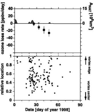
In Figure 2 (top panel) the temporal evolution of

the vortex-averaged ozone loss rate per day in the 475 K isentropic level is shown. Each data point includes

'• 20

ß

0

_o -40

Date [day of year 1998]

o

o

Figure 2. (top) Ozone depletion rates per day on the 475 + 10 K potential temperature level as a function of time. Each data point represents a linear regres- sion between ozone change and sunlit time of matches in a 14-day period around the given date. The shaded curve represents ANAT, the area with temperatures be-

low TNAT. (bottom) Relative position of the corre-

sponding match events inside the polar vortex. Zero

refers to the vortex center (highest PV value), while 1

represents the vortex edge. On a given day, equal inter- vals on the scale correspond to equal area fractions of the vortex, while decreasing numbers represent increas- ing PV (e.g., 0.3 represents the PV isoline enclosing

30% of the vortex area).

matches of a +7-day period around the given value. The shaded curve represents ANAT. The bottom panel shows the relative location of the contributing match events inside the polar vortex. Between mid January and the end of February, matches at 475 K cover the

polar vortex homogeneously (except for the innermost

20%); so the calculated loss rates can reasonably be

regarded as vortex averages. At this level, the vortex-

averaged loss rates do not exceed 10 4. 6 ppbv/d, which

is barely statistically significant. For comparison, the same analysis for the 490K isentropic level is shown

in Figure 3. Here loss rates reach clearly statistically

significant values in February.

Langer et al. [1999] deduced chemical ozone deple-

tion from ground-based millimeter wave observations of

ozone with a vertical resolution of $ kin, which at 475 K

roughly corresponds to 150 K vertical resolution. Loss

rates on the 475 K level were found to be not significant in December and the beginning of February. For the end

of February they give a loss rate of 32 4. 10ppbv/d or

7498 SCHULZ ET AL.' ARCTIC OZONE LOSS, 1997/1998 AND 1998/1999

E 550_

• 450

' '

[ppbv/day]

Date [day of the year 1998]

Plate 1. Ozone loss rates per day as a function of time and potential temperature. The thin solid lines indi-

cate the 0.3, 0.7, 1.5, 4.0, and 8.0.106 km 2 isolines for

the area with temperatures below TNA T as derived from ECMWF analysis. The dashed lines show the diabatic

descent (vortex average) of the air masses during the

winter as determined by the SLIMCAT model.

180øE

{;,

't,•,

8 :"

Plate 2. Synoptic temperatures at 475 K on February 18, 1998, from ECMWF analysis. The white line is the TNAT isoline, and the black line marks the isoline

of 36s -• normed potential vorticity, representing

the

vortex edge.

0

>8

• PEAK

[K]

..::

...

i

...

.-" :.,

...

.,"'

i ' -...:

, -..•,,__••

'"'""

.

...

.,,.

.

.• ."" ..-'" .'•;.'

2.,'•

'" ,•••.'•

•':•. .;.%%o

; :.,•

.... . , ;'...•..

7.0,:

.N_•.:,•.• .... '; ;:,{-,,,-•

i ...

...

....

:.;_:

... ...

: •.,.,. •.;- - . ,, ;..; .,,...'..;

•'•,.• •.•-"•.• -...,•

•,•:N

• ' ....:<'

;;"t,4:•

- .,.T'--•.-•

...t-./

...

_'..o;.

_{"•._.:}

_{. ---}

_{.-•'• .. •}

...

.•...':. . -

Plate 3. Map of the peak temperature amplitudes

of mountain

lee waves

•PEAK at 50 hPa on February

1998 at 1200 UT. The data are obtained by simulations

with a mountain wave forecast model [•c•e•ste•' et •.,

1994]. The blue contours are the synoptic temperature

= 40•

=o

0.8

•0.6

30

6'0

90

Date [day of year 1998]

15•

o;

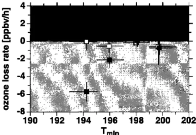
ary 10, and the solid squares include matches starting from February 10, which represent the same sample of matches as in Figure 4. Each match is assigned a min- imum temperature Tmi n as defined above. Here ozone loss rates per sunlit hour are calculated for ensembles of matches with a minimum temperature inside a 2 K wide bin. The horizontal lines mark the temperature bin; the horizontal position of the markers describe the average value of the individual minimum temperatures. A clear correlation between the minimum temperature and the ozone loss rate is observed for the February data, with a

maximum loss rate of 6 4- 1 ppbv/h for those air parcels

that experienced minimum temperatures between 193 and 195 K. It should be noted that these temperatures are synoptic temperatures. Owing to possible mesoscale temperature fluctuations, the temperatures given are upper limits of the lowest temperatures experienced by the air parcels.

Matches obtained in January and the beginning of

February (open squares) showed no ozone loss, includ-

ing those with minimum temperatures between 193 and

Figure 3. Same analysis as in Figure 2, but for the

490 4- 10 K potential temperature level.

the vortex-averaged rates we determine for the same period around 450 K and around 490 K.

To study the localization of the ozone depletion, the matches between February l0 and March 10 and be- tween 430 K and 500 K potential temperature (covering the region with significant loss rates) were chosen and binned according to their relative position inside the

vortex. In Figure 4 (top panel), the loss rates per sun-

lit hour calculated from this subset of match events are shown as a function of the relative location inside the vortex. The loss rates thus determined are small or zero

throughout most of the vortex but significant at the vor- tex edge, where ozone loss rates of 64-2 ppbv/sunlit hour

are reached. In Figure 4 (bottom panel), the minimum

temperatures (Train) in the history of the correspond- ing air parcels are shown. Tmi n iS defined as the low- est temperature found along a 10-day backward trajec- tory from the first sounding of the respective match and along the trajectory that links the two soundings. The averages of the minimum temperature are above

TNAT (dashed line) for all parts of the polar vortex, but

individual air parcels experienced lower temperatures, especially at the vortex edge. Since the higher loss rates observed in February 1998 are found at the vortex edge, where mountain wave activity is to be expected owing

to the geographical distribution of high mountains, the

influence of mesoscale temperature reductions leading

to PSC formation and hence ozone destruction as dis-

cussed by Carslaw et al. [1998] seems possible.

Figure 5 shows ozone loss rates for matches with dif-

ferent temperature histories. The open squares include matches from the beginning of January until Febru-

202- _ 2OO- _ 198- _ 196- 194- _ 192- _ 190 0 vortex center 0.2 I ' I 0.4 0.6 vortex edge I i O.8 I relative location

Figure 4. (top) Ozone loss rates per sunlit hour as

a function of relative location (see Figure 2 for an ex- planation) inside the vortex. The data symbolize linear regressions of matches between February l0 and March 10, 1998, and between 430 K and 500 K, each of them including matches of a 4-0.1 range around the given rel-

ative location. (bottom) Corresponding average of the

minimum temperatures Tmin for air parcels contribut- ing to loss rate calculations. For each matching pair of sondes, Tmin represents the lowest temperature on a 10-day backward trajectory from the first sounding and the trajectory which links the two soundings. Vertical lines indicate the range of the Tmin values.

7500 SCHULZ ET AL.' ARCTIC OZONE LOSS, 1997/1998 AND 1998/1999 o N 0 4 2 0 -2 _ -4 -6 -8 190 192 194 196 198 200 202 Tmin

Figure 5. Ozone loss rates for different minimum tem- peratures Tmi n in the air parcel histories as defined in Figure 4. Open squares include the data from January 1 until February 10; solid squares include those from February l0 until the end of the campaign in mid March 1998. The horizontal position of the markers is deter- mined by the average Tmin; the horizontal line marks the limits of the Tmi n values included in the data point.

195 K in the 10-day history. The average time spent below 195 K for the 43 trajectories in the earlier period

(open squares) with the lowest Tmi n is 12 hours, with 6

of those hours being between the two match soundings. This is comparable to the 13 trajectories in the later pe-

riod (solid squares), that on average encountered tem-

peratures below 195 K for 6 hours, 5 of them between the soundings. As was observed in other, colder Match winters, Tmi n values between 192 K and 195 K do not

necessarily lead to major ozone loss at 475 K [Schulz

et at., 2000b], suggesting that mesoscale temperature

fluctuations are needed to actually trigger ozone loss for Tmin values in this range. The possible influence of orographic lee waves on the observed ozone loss in February is discussed below.

Eleven of the 13 air parcels with considerable ozone loss experienced their lowest temperatures between 480 K and 500 K potential temperature above Scandinavia between February 17 and February 19, either between the two ozone soundings or shortly before the first sounding. None of these 11 encountered temperatures below 195 K in the rest of the 10-day backward trajec- tory. In Plate 2 the synoptic temperatures at 475 K are shown for February 18. The lowest temperatures are observed at the vortex edge above Scandinavia, where the white line indicates the TNA T isoline. In fact, PSCs

were observed by Lidar in Andoya (northern Norway)

on the night of February 16-17 (G. Hansen, private com-

munication, 2000), and none were observed at this loca-

tion on several other occasions in January and February. On February 17, PSCs were also observed at Sodankyl/i

(Finland) and were between 18.5- and 19.5-km altitude,

including a thin layer of solid PSC type I (R. Kivi, pri-

vate communication, 2000). This altitude range cor-

responds roughly to 440-465 K, as inferred from ra-

diosonde data, which is slightly lower than the ensem-

ble of matches discussed here (480-500 K). However,

the relation between geometrical height and potential temperature is highly variable within a lee wave event, which makes the comparison difficult.

It is therefore likely that this ensemble of air parcels experienced chlorine activation between February 17 and February 19 above Scandinavia. Model simulations

with a mountain wave forecast model [Bacmeister et at.,

1994] indicate that between February 17 and February

19 the lowest temperatures at 50 hPa coincided with high mountain wave activity above the Scandinavian mountains, which was not the case on the days before or after. Plate 3 shows the simulation for February 18, 1200 UT, at the 50-hPa pressure level. This indicates that the true minimum temperatures seen by these air parcels may have been significantly lower than that in- dicated in Figure 5, and that lee waves might have been responsible for this observed ozone loss.

The corresponding data point of the early period

(open squares) in Figure 5 showing no ozone loss in-

cludes 43 matches that are not confined to a small ver-

tical region but are distributed vertically between 430 K and 500 K. The air parcels experienced their lowest temperatures at different times and locations and there- fore cannot be brought in connection with any single lee wave event. However, mountain wave induced PSCs

have been observed in January 1998 [Behrendt et at.,

2000; R. Kivi, personal communication, 2000], and the

Match results at 475 K give indications for slight ozone

loss in January (Figure 2); so it is likely that small-

scale ozone loss confined to limited vertical regions also occurred in January.

3.2. Winter 1998/1999

The winter 1998/1999 was the warmest Arctic strato-

spheric winter examined with the Match technique so far. During most of the winter the stratospheric temper- atures were well above TNAT, and orographic lee wave activiy was weak and cannot be expected to have low- ered the temperatures enough for PSCs to form. To our knowledge, the only PSC measurements were made

on December 2 in Sodankylii [Kivi et al., 2000] be-

tween 545 K and 590 K. Visual observations were made

at Kiruna, Sweden during the December 1-3 period

[S. Kirkwood, private communication, 2000]. Figure 6

(top panel) shows the temporal evolution of the vortex-

averaged ozone loss rate per day in winter 1998/1999

at 475K. No statistically significant ozone loss was observed. There was only one short period in mid February when temperatures were below TNAT in the Northern Hemisphere. However, no Train values below 195 K are found among the matches used for this anal-

ysis (Figure 6, middle panel), indicating that the small

geographical region with synoptic temperatures below TNAT was not sampled with Match during the time of interest. Small-scale ozone loss induced by this colder

• -20 -40 -60 210 205

200

ß

'•

ß

Date [day of year 1999]

i

Figure 6. (top) Ozone loss rates per day in the 475-+-10 K potential temperature level as a function of time for early 1999. Each data point represents a linear regres- sion between ozone change and sunlit time of matches in a 14-day period around the given date. (middle) Corresponding Tmi n values of air parcels. The vertical position of the marker is the average Train, the verti- cal line represents the range of the individual Tmi n val-

ues. (bottom) relative position of corresponding match

events inside the polar vortex (see Figure 2 for an ex- planation).

event may have been missed by Match. Still, the obser- vation of no ozone loss stands out from the preceding winters with significant ozone loss and provides further experimental evidence that the present chlorine load- ing in the Arctic stratosphere does not necessarily lead to chemical ozone loss, provided the temperatures are high enough. At 475 K, the average temperature in the coldest 20% of the vortex during January, February and March 1999 was 2044-5 K, which is 6 K higher than that in 1998 and 8-10 K higher than that in 1995, 1996 and 1997. These temperature differences remain even when other quantities such as the minimum tempera- ture inside the vortex or the mean vortex temperature are compared.

Corresponding to the absence of major chemical ozone

loss, the observed ozone mixing ratios in winter 1998/

1999 were unusually high in comparison with recent preceding winters. The average mixing ratio in Febru- ary and March at 475 K inside the polar vortex was 3.7 4. 0.3 ppmv and 3.8 + 0.3 ppmv, as calculated from

all sondes with a normed P V value higher than 30 s -1

and PV _• 36s -1, respectively. For comparison, the

vortex-averaged

(PV _• 36 s -•) values

for February

and

March of former years were 3.1 4. 0.4 ppmv in 1997 and 3.0 4. 0.3 ppmv in 1998.

4. Conclusion

The 1997/1998 Match results give a detailed picture of chemical ozone loss ra•es in •he Arctic stratosphere with respect to time and altitude and •o relative lo- cation inside the vortex. In 1997/1998 stratospheric temperatures were relatively high. They were close to TNAT for a long period and occasionally dropped below TNAT for a couple of days. This situation offered the un- precedented opportunity to study the chemical ozone loss under •hreshold conditions. The vortex-averaged ozone loss rates were barely significant for most of the winter throughou• rnos• of the vortex. Some clearly significan• ozone loss occurred in February mainly con- fined to the vortex edge. This may have been connected •o local PSC formation in lee wave events. The high- es• loss ra•es in February were observed in •hose air parcels wi•h minimum •ernpera•ures below 195 K be- tween •he •wo soundings or in a 10-day history prior to the first ozonesonde. In 1998/1999, temperatures stayed well above TNAT and no significant ozone loss was observed. Compared with earlier winters during the 1990s, the absence of substantial ozone loss during these two relatively warm winters shows how sensitive the chemical ozone loss is to changes in stratospheric temperature. As a rough estimate, the Match results show that a mean stratospheric temperature increase of 2-4 K inside the polar vortex can account for the dif-

ference between severe ozone loss and ozone loss that

is confined to sporadic events such as those in winter

1997/1998, while a temperature increase of 8-10 K with

respect to a situation with substantial ozone loss led to no chemical ozone depletion. These observations sup- port the hypothesis that during the next decades, while

the chlorine loading is still expected to be high [World

Meteorological Organization, 1999], the evolution of the

stratospheric temperatures will be the determining fac-

tor for the amount of wintertime chemical ozone loss in

the Arctic stratosphere.

Acknowledgments. We are grateful to the operating staff of all participating stations for having made these cam- paigns possible. We thank H. Deckelmann, AWI Potsdam, for computer work, as well as the the European Centre for Medium-Range Weather Forecast (ECMWF) and the Ger- man Weather Ofiqce (DWD) for providing meteorological data. This work was supported by the European Commis-

7502 SCHULZ ET AL.: ARCTIC OZONE LOSS, 1997/1998 AND 1998/1999

sion

within the project

THESE(J-O31oss,

contract

ENV4-

References

Bacmeister, J. T., P. A. Newman, B. L. Gary, and K. R. Chan, An algorithm for forecasting mountain wave- related turbulence in the stratosphere, Weather Forecast- ing, 9, 241-253, 1994.

Behrendt, A., J. Reichardt, A. DSrnbrack, and C. Weitkamp,

Leewave PSCs on northern Scandinavia between 22 and

26 January 1998: Lidar measurements of temperature and optical particle properties above Esrange and mesoscale model analysis, in Proceedings of the Fifth European Work- shop on Stratospheric Ozone, St. Jean de Luz, France, 27 September to i October 1999, pp. 149-152, European Commission, Brussels, 2000.

Carslaw, K. S., M. Wirth, A. Tsias, B. P. Luo, A. DSrnbrack, M. Leutbecher, H. Volkert, W. Renger, J. T. Bacmeister, and E. Reimer, Increased stratospheric ozone depletion due to mountain-induced atmospheric waves, Nature, 391, 675-678, 1998.

Chipperfield, M.P., Multiannual simulations with a three- dimensional chemical transport model, J. Geophys. Res., 10J, 1781-1805, 1999.

Hanson, D., and K. Mauersberger, Laboratory studies of the nitric acid trihydrate: Implications for the south polar stratosphere, Geophys. Res. Lett., 15, 855-858, 1988. Kivi, R., et al., in Proceedings of the Fifth European Work-

shop on Stratospheric Ozone, St. Jean de Luz, France, 27 September to i October 1999, pp. 169-172, European Commission, Brussels, 2000.

KyrS, E., H. Aulamo, R. Kivi, and T. Turunen, Changes in Arctic polar vortex, in Proceedings of the Quadrennial Ozone Symposium, Sapporo, Japan, July 3-8, 2000, pp. 509-510, National Space Development Agency of Japan, Tokyo, 2000.

Langer, J., B. Barry, U. Klein, B.-M. Sinnhuber, I. Wohlt- mann, and K. F. Kiinzi, Chemical ozone depletion dur- ing Arctic winter 1997/98 derived from ground based millimeter-wave observations, Geophys. Res. Lett., 26, 599-602, 1999.

Manney, G. L., L. Froidevaux, M. L. Santee, R. W. Zurek, and J. W. Waters, MLS observations of Arctic ozone loss in 1996-97, Geophys. Res. Lett., 2J, 2697-2700, 1997. Mfiller, R., J.-U. Groofi, D. S. McKenna, P. J. Crutzen, C.

Briihl, J. M. Russell III, and A. F. Tuck, HALOE observa- tions of the vertical structure of chemical ozone depletion in the Arctic vortex during winter and early spring 1996- 97, Geophys. Res. Lett., 2J, 2717-2720, 1997.

Pawson, S., and B. Naujokat, The cold winters of the mid- dle 1990s in the northern lower stratosphere, J. Geophys. Res., 10•, 14209-14222, 1999.

Rex, M., et al., Prolonged stratospheric ozone loss in the 1995-96 Arctic winter, Nature, 389, 835-838, 1997. Rex, M., et al., Chemical ozone loss in the Arctic winter

1994/95 as determined by the Match technique, J. Atmos. Chem., 2•, 35-59, 1999.

Schulz, A., et al., Match observations in the Arctic win- ter 1996/97: High stratospheric ozone loss rates correlate with low temperatures deep inside the polar vortex, Geo- phys. Res. Left., 27, 205-208, 2000a.

Schulz, A., et al., Chemical ozone loss rates in the Arctic stratosphere and their dependence on temperatures as de- termined with Match, in Proceedings of the Quadrennial Ozone Symposium, Sapporo, Japan, July 3-8, 2000, pp. 103-104, National Space Development Agency of Japan, Tokyo, 2000b.

von der Gathen, P., et al., Observational evidence for chem- ical ozone depletion over the Arctic in winter 1991-92, Nature, 375, 131-134, 1995.

World Meteorological Organization, Scientific assessment of ozone depletion: 1998, Rep. 44, Geneva, 1999.

R. Alfier and E. Reimer, Meteorological Institute, FU Berlin, C.-H.-Becker Weg 6-10, D-12165 Berlin, Germany. (alfier@strat04.met.fu-berlin. de; reimer@fub46.zedat.fu- berlin.de)

M. Allaart, KNMI, P.O. Box 201, 3730 AE De Bilt, Netherlands. (allaart@knmi.nl)

M. Alpers, IAP, Schlofistr. 6, 18221 Kfihlungsborn, Germany. (alpers@iap-kborn. de)

B. Bojkov and G. O. Braathen, NILU, P.O. Box 100, Instituttveien 18, N-2007 Kjeller, Norway.

(bojan.bojkov@nilu.no; geir@nilu.no)

J. Cisneros, Instituto Nacional de Meteorologia, Apdo. 285, 28071 Madrid, Spain. (Juan. Cisneros@inm.es)

H. Claude, DWD, Observatory Hohenpeifienberg, Albin- Schwaiger-Weg 10, 82383 Hohenpeifienberg, Germany. (h ans. clau de@ dwd. de)

E. Cuevas, Instituto Nacional de Meteorologia, Tenerife, Spain. (ecuevas@inm.es)

J. Davies and H. Fast, Atmospheric Environment Service, 4905 Dufferin Street, Downsview, Ontario, M3H 5T4, Canada. (Jonathan. Davies@ec.gc.ca; Hans. Fast@ec.gc.ca)

H. De Backer, Royal Meteorological Institute, Ringlaan 3, B-1180 Brussels, Belgium. (Hugo. DeBacker@oma.be)

H. Dier, Meteorologisches Observatorium Lindenberg, 15864 Lindenberg, Germany. (dier@mol.dwd.d400.de)

V. Dorokhov and V. Yushkov, CAO, Pervomajskaya Street 3, Dolgoprudny, Moscow Region, 141700, Russia.

(vdor@ozone.mipt.ru; vladimir@ozone.mipt.ru)

S. Eckermann, E. O. Hulburt Center for Space Research, Code 7641, Naval Research Laboratory, Washington DC • 20375-5352. (eckerman@ismap4.nrl.navy. mil)

S. Godin, Universit• Paris 6 Service d'A•ronomie du CNRS, 4 Place Jussieu Paris Cedex 05, 75230 France. (sg@aero.jussieu.fr)

N. R. P. Harris and I. Kilbane-Dawe, EORCU, 14 Union Road, Cambridge, CB2 1EW, United Kingdom. (Neil'Harris@øzøne-sec'ch'cam'ac'uk; Iarla. Kilbane-Dawe@ ozo n e-sec. ch. cam. ac. uk)

B. Johnson, NOAA/CMDL Ozone and Water Vapor Group, 325 Boulder, CO 80303-3328. (bjohnson@cmdl.noaa.gov)

B. Kois and Z. Litynska, Institute of Meteorology and Water Management, Centre of Aerology, Zegrzynska Str.38, 95-119 Legionowo, Poland. (kois@pol.pl; zenoblit@pol.pl)

Y. Kondo, Research Center for Advanced Science and Technology, University of Tokyo, 4-6-1 Komaba, Meguro-ku, Tokyo 153-8904, Japan. (kondo@atmos.rcast.u- tokyo.ac.jp)

E. Kosmidis and C. Zerefos, Laboratory of Atmospheric Physics, University of Thessaloniki, 45006 Thessaloniki, Greece. (ekøsmidi@auth'gr; zerefos@ccf. auth.gr)

E. KyrS, Sodankyl•i Meteorological Observatory, T•ihte- l•intie 71, 99600 Sodankyl•i, Finland. (Esko. Kyro@fmi.fi)

I. S. Mikkelsen, Danish Meteorological Institute, Lyng-

byvej 100, DK-2100 Copenhagen, Denmark. (ism@dmi.dk) M. J. Molyneux, The Meteorology Office, (OLA)3b, BeaUfort Park, Wokingham, Berkshire, RG40 3DN, United Kingdom. (mjmolyneux@meto.gov.uk)

G. Murphy, IMS, Valentia Observatory, Cahirciveen, County Kerry, Ireland. (gamurphy@iol.ie)

T. Nagai, Meteorological Research Institute, 1-1 Nagamine, Tsukuba, Ibaraki 305-0052, Japan. (tnagai@mri-jma'gø'JP)

H. Nakane, National Institute for Environmental Studies, 16-20nogawa, Tsukuba, Ibaraki 305-0053, Japan.

(nakane@nies.go.jp)

F. O'Connor, Centre for Atmospheric Science, Cambridge University, Lensfield Road, Cambridge CB2 1EW, United Kingdom. (Fiona. O Connor@atm.ch.cam. ac.uk)

C. Parrondo, INTA, Torrejon de Argoz, 2885'0 Madrid, Spain. (parrondosc@inta.es)

M. Rex, A. Schulz and P. von der Gathen, Alfred Wegener Institute for Polar and Marine Research, P.O. Box 600149, 14401 Potsdam, Germany. (mrex@awi-potsdam.de; aschulz@awi-p orsdam.de; gathen@awl-potsdam. de)

F. J. Schmidlin, Laboratory for Hydrospheric Processes, NASA GSFC/Wallops Flight Facility, Wallops Island, Virginia 23337. (fjs•osbl.wff. nasa.gov)

P. Skrivankova Czech Hydrometeorological Institute, Up- per Air and Surface Observation Department, Na Sabatce 17, 143 06 Prague, Czech Republic. (skrivankova@chmi.cz)

C. Varotsos, University of Athens, Department of Applied Physics, Panepistimioupolis Building PHYS-V, 157

84 Athens, Greece. (kvarots@atlas.cc.uoa.gr)

C. Vialle, IPSL/Service d'Observation, BP 3, 91371 Verri•res le Buisson, Cedex, France.

( Claude. Vialle@aerov.jussieu.fr)

P. Viatte, SMI, Les Invuardes, 1530 Payerne, Switzer- land. (pvi•sap.sma.ch)

(Received June 13, 2000; revised September 19, 2000;