Development of a combined multi-sensor/signal processing architecture for improved in-situ quantification of the charge balance of natural waters

(1)

Development of a Combined Multi-Sensor/Signal Processing

Architecture for Improved In-Situ Quantification of the

Charge Balance of Natural Waters

by

Amy Violet Mueller

Submitted to the Department of Civil and Environmental Engineering in partial fulfillment of the requirements for the degree of Doctor of Philosophy in the Field of Environmental Chemistry

at the

MASSACHUSETTS INSTITUTE OF TECHNOLOGY June 2012

Author . . . . Department of Civil and Environmental Engineering

May 4, 2012

Certified by . . . . Harold F. Hemond William E Leonhard Professor of Civil and Envrionmental Engineering Thesis Supervisor

Accepted by . . . . Heidi M. Nepf Chair, Departmental Committee for Graduate Students

(2)

(3)

Development of a Combined Multi-Sensor/Signal Processing Architecture for Improved In-Situ Quantification of the Charge Balance

of Natural Waters by

Amy Violet Mueller

Submitted to the Department of Civil and Environmental Engineering on May 4, 2012, in partial fulfillment of the

requirements for the degree of

Doctor of Philosophy in the Field of Environmental Chemistry

Abstract

This thesis details the design, implementation, and testing of a new electrochemical instru-ment for the in situ measureinstru-ment of both major and environinstru-mentally relevant minor ions in fresh waters, namely Na+, K+, Ca2+, Mg2+, NH₄+, Cl−, NO−₃, and SO2−₄ . The instru-ment is built on a hybrid multi-probe / signal processing architecture and is impleinstru-mented using commercial sensor hardware (primarily ion-selective electrodes (ISEs)) paired with a novel neural network processor designed to take advantage of a priori chemical knowledge about the system. Adaptation of this architecture to in-situ conditions and quantifica-tion of relatively minor ions required overcoming a number of challenges, including: (1) lack of a standardized method for unsupervised recording of ISE equilibrium potential, (2) non-availability of commercial electrodes for some ion species, and (3) detection of ion con-centrations that fall below the ISE linear response region and/or are confounded by the presence of relatively large quantities of interfering ions. As such, a methodology is pro-posed and validated for standardization of ISE potential readings, resulting in consistent measurements completed in <6.5 min., improving replicability, and facilitating simultane-ous measurement of up to 12 ion channels. The sensor suite is then designed such that each ISE provides information about more than one analyte, and finally, the artificial neural network (ANN) architecture is optimized for use on environmental chemical data by includ-ing software constraints implementinclud-ing known chemical relationships, i.e., the concept of charge balance and the total ion-conductivity relationship. Two experiments are conducted using environmentally-relevant data sets (one semi-synthetic, one created in the lab) to characterize the effectiveness of the proposed ANN architecture. Final results demonstrate over an order of magnitude decrease in relative error (as measured against use of ISEs as stand-alone sensors) without concentration-dependent error bias, including estimates for analytes for which no specific ISE exists (SO2−₄ , Mg2+, HCO−₃). Simultaneous un-biased quantification of all eight ions is achieved with ˜20% error on most channels including NO−₃ (concentrations ≤100 µM) and ˜50% error for NH+₄ (≤100 µM), however it is also demon-strated that errors of ˜10% are achievable for N-species ions even at low concentration if slightly higher uncertainties on other channels can be tolerated.

Thesis Supervisor: Harold F. Hemond

(4)

(5)

Acknowledgments

What we all conclude about science after realizing most of our advisors finished their PhD in fewer years than we took to complete undergrad. Image updated from boasas.com I would first and foremost like to thank my advisor, Harry, for all of his advice, direction, and understanding over the years. It is, I believe, a unique and yet universal experience for each of his students to explore his seemingly boundless expertise, testing the waters with ever more difficult or unstudied questions and concepts, with the hope of one day catching up to his subtle and modest intuition for just about everything - and even five, six, or seven years into this process, it is each time somehow simultaneously maddening and reassuring to realize that he had a handle on the crux of the matter well before you even bothered to put the question to him. I consider myself extremely lucky to have had the honor to work with him on this and a number of other projects over the past 8 years, as I have most certainly become a more effectively inquisitive scientist and productive engineer under his guidance.

Similarly Professor Phil Gschwend has been instrumental in teaching me about how to conceptualize my work, distill it down to its meaningful essence, and present it to people in a way that they can understand and - perhaps most importantly - put into context within the vast space that environmental engineering covers. Phil has also taught me how to be a good audience member, how to ask good questions, and how to think about other people’s research critically, and for this I am extremely grateful.

And to the whole of the Parsons Supergroup - especially those individuals who saw me through my first few years on this project - I owe all of you for the consistent source of great suggestions, patient ears when my setup was going wonky, and for providing a safe place to talk about research failures as well as successes. I still don’t love public speaking, but being able to talk about my work to this wonderful group of people has bolstered me up to the point where I can buck up and get through it without the knock-kneed butterfly stomach I had 8 years ago at just the thought of giving talks.

I must also thank my parents, who probably thought I was crazy for going back to school again but have been nothing but supportive along the way, and my brothers, who have made being back in Boston a whole lot of fun. As a side note, Dad, thank you for

(6)

acclimating me to the sound of construction at such a young age - it has been key to the completion of a massive amount of this work and writing during the complete renovation of the room next door over the past 6 months. Next is a long list of friends - some who have known me for almost 20 years at this point and some found recently - who must be credited with helping me keep hold of my sanity in dire straits (and for humoring my rants about tiny details of my research with a straight face and a lot of patience). My sanity has also been secured through the cheerful and consistent guidance of Checka, the most wonderful of yoga instructors, who taught me to keep the big picture in mind and strive always for Focus, Communication, Patience, and Contentment. And finally Matt - thank you for adding adventures into the mix and reminding me that there is more life out there waiting to be experienced and humanity out there waiting to be helped. Olyan boldog vagyok hogy egymast vigyazunk et hogy te vagy az enyem.

There are also a number of researchers whose work has been inspirational to me, helped me to formulate this project from a wee inkling of an idea into something with a chance of actually seeing the light of day, and taught me volumes about the hardware, software, applications, and context of this project. Since I first stumbled on their trails, I have been actively chasing down just about anything they published and been the better scientist for it, so I wanted to take this opportunity to acknowledge their contributions (and those of their students) to my work: E. Bakker, E. Pretsch, M. del Valle, S. Alegret, Y. Vlasov, A. Legin, C. DiNatale, A. D’Amico, and W. Morf. Thank you for being shoulders I could stand on.

And finally, though they will probably never know how grateful I am, I want to thank the individuals out there who put in the time to catalog tables of seemingly esoteric chemical data or to painstakingly explain obscure Matlab functions in help forums so that I could stumble across it through desperate internet searches. Random folks: you saved me a whole lot of time, and I really appreciate it. If it weren’t for you, who knows how much longer this thesis could have taken...

(7)

List of Figures

2-1 Ion selective electrode cell [1]. . . 24

2-2 Binding free energy (kJ·mol−1) for alkali metals with a series of cryptand and 18-crown-6 ionophores, from [2]. . . 26

2-3 CHEMFET cross section [3]. . . 28

3-1 Photographs of lab setup for ISE sampling, including ISE hardware (orange), custom circuitry (yellow), data acquisition (teal), and PC for LabView inter-face (far left). . . 43

3-2 Wiring diagram for BNC interfaces from ISEs to isolation hardware. . . 44

3-3 Two-pole Butterworth filter. . . 45

3-4 Isolation input / low-pass filter circuit schematic. . . 47

3-5 Isolation input / low-pass filter PCB. Red traces are on the top layer of the PCB while green traces are on the bottom layer. Black encodes component outlines and text printed on the PCB screenprint layer. . . 48

3-6 LabView user interface. . . 48

3-7 LabView schematic for data acquisition. . . 49

4-1 Typical non-monotonic ISE response signal as seen in this study (left) and as elucidated by Lindner et al. [4] (right). . . 54

4-2 Range of time-series responses of ion selective electrodes to a single aqueous sample. . . 55

4-3 Mean percent change in determined steady state concentration for the tighter range of parameterizations relative to the baseline case of { 0.4 mV·min−1, 30 sec }. Interior solid bars show the mean change (black: > 0; red: < 0) while exterior transparent bars show the mean absolute value of the change. Note that parameterization difference within this range can results in no more than 0.6% change in declared concentration. . . 57

4-4 Mean absolute change in determined steady state emf [mV] for a range of parameterizations relative to the baseline case of {0.4 mV· min−1 , 30 sec}. Difference in bar heights indicates that emf declared for a specific time series may vary significantly with parameter choice. . . 60

4-5 Calibration curves for four ELIT ISEs in their respective salts (3σ error bars). Linear fits with near-Nernstian slopes (Nernstian slope at measurement tem-perature of 19°C is 57.9) and R2 > 0.99 are found for concentrations down to 1µM in all cases (down to 0.25µM for K+). . . 61

(12)

4-6 Effect of parameterization on equilibrium failure rate, λfaiure, for a sample

period of ˜6.5 minutes. Bars are subdivided by solution content (A) and probe (B) to demonstrate the range of characteristics affecting the response time of electrodes. . . 62 4-7 Summary of parameterization ‘goodness’ as judged by simultaneous

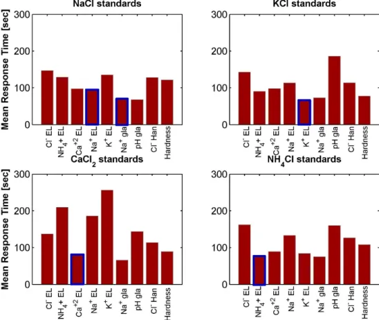
mini-mization of RMSE and maximini-mization of equilibrium success rate. Cross-hatching = poor results; * = good results for all probes; M/U = good results for the subset of selectivity matched (M) or un-matched (U) salt/ISE probe pairs. . . 63 4-8 Mean difference in determined response time [sec] relative to the {0.4mV·

min−1 , 30 sec} baseline over a range of parameterizations; plot on the right shows results for a more constrained parameterization set (referenced to plot on left). Blue tones indicate that parameterization produces shorter response times than baseline while red tones indicate longer response times (note color-bar scale change from left to right). Note total difference of almost 3 minutes across parameterizations shown in plot on left as compared to a difference of less than 1 minute on the right. . . 64 4-9 Effect of electrode sensitivity and membrane type on mean response time for

baseline parameter values. . . 65 4-10 Response time averaged over 9 electrodes for different salt solutions at a range

of concentrations. Data are taken for parameter values {0.4 mV·min−1, 30 sec}. . . 66 4-11 Response time of independent electrode channels as a function of NaCl or

KCl concentration. Data are taken for parameter values {0.4 mV·min−1, 30 sec}. . . 67 4-12 Response time of independent electrode channels as a function of CaCl2 or

NH4Cl concentration. Data are taken for parameter values {0.4 mV·min−1,

30 sec}. . . 68 5-1 Prototypical neuron component of a neural network. Figure courtesy of the

MathWorks. . . 72 5-2 Overview of neural network training. Figure from [5]. . . 73 5-3 Matlab-formatted representation of three neural network architectures: a

traditional structure (top), one with a single constraint layer (middle), and one with two constraint layers (bottom). (Note that the middle case is la-beled EC for the Electrical Conductivity case but could represent either of the chemical constraints discussed here.) Weights and biases omitted from training in the non-traditional architectures are boxed in red, while nodes where Matlab applies the mapminmax (or inverse) function are highlighted in yellow. . . 75 6-1 Electrode response to a range of salts. (Top) Response of the ELIT Na+

ISE to four cations. (Bottom) Response of 9 electrodes to different concen-trations of NH4Cl solution. Note that log-linear responses exist for most

ISE/ion pairs, indicating that use of these electrodes in mixed-salt solutions will produce responses due partially to each of the ionic constituents. . . 86 6-2 Direct comparison of MA and TX data ‘fingerprints’. . . 87

(13)

6-3 Ionic characteristics of Massachusetts (left) and Texas (right) data selected for simulated data set. . . 87 6-4 Basic feedforward ANN structure used as the starting point for training. . . 88 6-5 Inclusion of charge balance constraint via addition of a non-trained output

layer in the ANN. Hidden and output layers shown on the left refer to those included in the generic feedforward ANN structure shown in Fig. 6-4. . . . 89 6-6 Improvement in prediction of MA concentrations using a MA-trained ANN

with both conductivity and charge balance constraints. Results are shown relative to use of ISEs as stand-alone (single analyte) sensors. . . 91 6-7 Concentration prediction results using a MA+TX trained ANN to process

both MA and TX data. . . 93 7-1 One-dimensional probability distribution functions for representative

envi-ronmental ions, created using archived USGS data for the five states listed. Density values are plotted at bin mid-points. . . 97 7-2 Cumulative distribution function for 8-D ion Joint PDF. Independent axis is

a sorted bin index, with bins sorted by descending density contribution. . . 98 7-3 Mean response of divalent ISEs as a function of primary analyte concentration.101 7-4 Mean response of monovalent ISEs as a function of primary analyte

concen-tration. . . 103 7-5 Estimated EC based on ion makeup of water samples as compared to

mea-sured EC (temperature corrected and calibrated). Measurements from VWR meter were highly correlated with but consistently lower than those produced by the Amber meter; it is expected this is related to the built in temperature correction software which was disabled for these experiments but does not always completely disable correctly. . . 104 7-6 ISE-based predictions of ion concentrations (prediction vs. target) for NH+₄,

NO−₃, Na+, and Cl−. Limit of detection (LOD) is plotted as a vertical dotted line. . . 107 7-7 ISE-based predictions of ion concentrations (prediction vs. target) for K+,

Ca2+_{, hardness, and SO}2−

4 . Limit of detection (LOD) is plotted as a vertical

dotted line. . . 108 7-8 Total NRMSE as a function of ANN architecture. Horizontal axis shows

output configuration while colored bars represent options for data used in training (mix data only / mix data plus single-salt standards) and data nor-malization (none / log). . . 114 7-9 Relative percent error for optimal ANN predictions as a function of analyte

concentration. Results are shown for mix data only. . . 116 7-10 Scatter plots of nitrogen ion concentrations predicted using the optimal ANN

as a function of target concentration. One-to-one line shown in red; regression of estimates against targets (concentration data) and 95% confidence interval on the linear fit shown in black. . . 117 7-11 Scatter plots of Na+ and Cl− ion concentrations predicted using the

opti-mal ANN as a function of target concentration. One-to-one line shown in red; regression of estimates against targets (concentration data) and 95% confidence interval on the linear fit shown in black. . . 118

(14)

7-12 Scatter plots of K+ and Ca2+ ion concentrations predicted using the opti-mal ANN as a function of target concentration. One-to-one line shown in red; regression of estimates against targets (concentration data) and 95% confidence interval on the linear fit shown in black. . . 119 7-13 Scatter plots of Mg2+ and SO2−₄ ion concentrations predicted using the

opti-mal ANN as a function of target concentration. (Note most ISE predictions do not fit on graph at this scale.) One-to-one line shown in red; regression of estimates against targets (concentration data) and 95% confidence interval on the linear fit shown in black. . . 120 7-14 Scatter plots of carbonate system ion concentrations predicted using the

op-timal ANN as a function of target concentration. Note that there is sig-nificant bias in these estimates at increasingly small concentrations; it is expected that improvement in sulfate concentrations (which have the similar magnitude contribution as carbonate concentrations in the charge balance equation) would further reduce the uncertainty in these low-concentration predictions, while the same can be stated for further simultaneous improve-ment of bicarbonate and chloride predictions. One-to-one line shown in red; regression of estimates against targets (concentration data - note low con-centrations do not contribute significantly to this fit) and 95% confidence interval on the linear fit shown in black. . . 121 7-15 Scatter plot of constraint predictions of optimal ANN as a function of target

value. One-to-one line shown in red; regression of estimates against targets (data before log-transformation) and 95% confidence interval on the linear fit shown in black. . . 122 A-1 Ion concentrations in 75 training samples, plotted against sample number.

Recall that ‘low’ and ‘high’ nitrogen conditions were imposed on, respectively, samples 26-50 and samples 51-75. . . 130 A-2 Response of ELIT ISEs to each of five single-salt calibration standards. . . 134 A-3 Response of glass and divalent cation ISEs to each of five single-salt

calibra-tion standards. . . 135 A-4 Response of anion ISEs to each of five single-salt calibration standards. . . 136 A-5 Relvative error (as %) for ISE-based predictions of ion concentrations. . . . 141 A-6 Correlation of net goodness parameters with error calculations for nitrogen

ions. . . 142 A-7 Scatter plots of ion concentrations predicted using the optimal ANN (chosen

(15)

List of Tables

2.1 Sensor types used for measurements of relevant ions. . . 25 3.1 Overview of commercially-available sensors of interest for this application

(accurate as of 2009; manufacturers such as WPI and YSI released some additional ISE-based instrumentation in 2010-11). Analytes listed are not comprehensive and are intended to be representative of quantities of interest for this application. . . 41 3.2 Sensor hardware incorporated into the sensor suite. . . 42 3.3 Physical layout of inputs to LPF Stage from Coax Plug Wall. . . 44 3.4 Physical layout of outputs from LPF Stage to Data Acquisition I/O Pins.

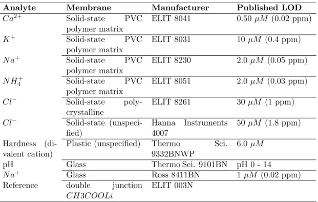
Note: * value connected to all ‘-’ inputs for used analog input ports. . . 45 4.1 Single-salt standards used for electrode characterization, producing a total

of 52 standard salt solutions. . . 58 4.2 Ion selective electrode hardware; information on membrane composition and

published detection limit (LOD) as given by manufacturers where available. 59 5.1 Neural network characteristics and parameters. . . 74 5.2 Charge balance and conductivity constraint multipliers used for calculation

of non-trained neuron weights. Conductance values adapted from [6, 7].

∗_{Note that the charge balance constraint has been formulated such that the}

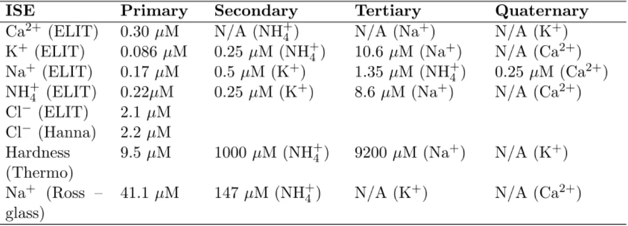
balance of all other ions is trained to the net contribution from H+ and OH− as explained further in the text. . . 78 6.1 Experimental Characterization of ISE limits of detection (LOD). Primary

refers to the ‘named’ ion of selectivity (e.g., Ca2+ for the ELIT Ca2+ ISE), while secondary, tertiary, and quaternary (analyte indicated in parenthesis after the LOD value) are ordered by response magnitude (mV·M−1) and not the LOD value. Note that Cl− was the only cation in this study (excepting OH− at low, fairly constant concentration) and thus does not have data for response to non-primary ions. . . 84 6.2 Data from USGS sites in Massachusetts [8]. . . 84 6.3 Data from USGS sites in Texas [8]. . . 85 6.4 Mean change in parameters, given as (simulated value - recorded value) for

chloride, conductivity, and hardness (percentage change relative to the mean of measurements is given in parentheses), resulting from the creation of the semi-synthetic data set from actual ionic data measured by the USGS. . . . 85 6.7 NRMSE comparison of MA+TX-trained ANN applied to (a) MA data and

(16)

6.5 NRMSE of analyte concentration predictions for MA data made using ISEs only (as stand-alone single-analyte sensors) and by using ISEs processed with the optimal ANN (minimization of NRMSE for these five analytes). Best predictions for each analyte are identified with bold font. . . 92 6.6 NRMSE comparison of MA-trained ANN results when applied to (a) MA

data and (b) TX data. Results are compared to (c) NRMSE for ISEs used as single-analyte sensors on TX data, and degradation in estimation perfor-mance is represented by (d) the ratio of NRMSE for TX data to NRMSE for MA data. . . 92 7.1 Approximate concentration ranges for ions of interest in New England waters

(log10[M]). . . 98

7.2 Salt solutions used in creation of ion mix samples (all standards at 100mM except for Ca(OH)2 and MgCO3 which were 20mM and 1.2mM respectively). 99

7.3 Required (for calculation of chemical constraints) and additional (quantities that can be calculated or inferred given provided information) target outputs for the neural network architecture. . . 102 7.4 Range of parameters explored for design of neural networks. . . 105 7.5 Formulae for metrics used to rank ANN results, including MSE (mean squared

error), NRMSE (normalized root mean squared error), MRE (mean relative error). . . 105 7.6 Range of parameters explored for design of neural network architecture. . . 106 7.7 Errors for ISE-based ion concentration predictions. . . 109 7.8 Parameterizations for best ANN (chosen using NRMSE metric) as a function

of ‘External’ architecture. . . 110 7.9 Concentration NRMSE and (MRE ) (as %, mean of absolute value of

rela-tive errors) for each of 8 target ions. ANN architecture defined by outputs (12 ions, 19 outputs, or 12 ions with 1 or 2 constraints) and error weight-ing on constraints (EW). Architectures trained to concentration values of mix data; optimal network (highlighted in left column) selected using the NRMSE metric. Optimal results for each concentration are individually highlighted in the corresponding columns. . . 112 7.10 Concentration NRMSE and (MRE ) (as %, mean of absolute value of

rela-tive errors) for each of 8 target ions. ANN architecture defined by outputs (12 ions, 19 outputs, or 12 ions with 1 or 2 constraints) and error weight-ing on constraints (EW). Architectures trained to concentration values of mix and single-salt data; optimal network (highlighted in left column) selected using the NRMSE metric. Optimal results for each concentration are individually highlighted in the corresponding columns. . . 112 7.11 Concentration NRMSE and (MRE ) (as %, mean of absolute value of

rela-tive errors) for each of 8 target ions. ANN architecture defined by outputs (12 ions, 19 outputs, or 12 ions with 1 or 2 constraints) and error weight-ing on constraints (EW). Architectures trained to logarithm-transformed mix data; optimal network (highlighted in left column) selected using the NRMSE metric. Optimal results for each concentration are individually high-lighted in the corresponding columns. . . 113

(17)

7.12 Concentration NRMSE and (MRE ) (as %, mean of absolute value of rela-tive errors) for each of 8 target ions. ANN architecture defined by outputs (12 ions, 19 outputs, or 12 ions with 1 or 2 constraints) and error weight-ing on constraints (EW). Architectures trained to logarithm-transformed mix and single-salt data; optimal network (highlighted in left column) selected using the NRMSE metric. Optimal results for each concentration are individually highlighted in the corresponding columns. . . 113 7.13 Parameterization of the linear regression of ANN-predicted concentrations

against target concentrations; in nearly all cases slope is statistically indis-tinguishable from 1 and intercept is statistically indisindis-tinguishable from 0. . 115 7.14 Ion concentration prediction errors for optimal ANN compared to results

using ISEs as stand-alone sensors. . . 115 A.1 Deliniation of bin edges (as log10(M)) for PDF based on USGS-recorded

environmental samples. . . 129 A.2 Ion concentrations (µM, except for alkalinity which is given in mM) for chosen

training sample mixtures. Recall that ‘low’ and ‘high’ nitrogen conditions were imposed on, respectively, samples 26-50 and samples 51-75; in some cases, equilibrium pH will lead to decrease in NH+₄ as equilibrium shifts toward NH3. Calculations are given for alkalinity, pH, and carbonate species,

for cases of (1) full equilibration with atmospheric CO2 (392 ppm, recorded

at Mauna Loa Dec. 2011) or (2) limited carbon exchange (carbonate system limited by standards used for sample creation). . . 131 A.3 Most informative calibration curve for prediction of target ions directly using

ISEs as stand-alone sensors . . . 137 A.4 Pairwise correlation coefficients between net (whole data set) goodness

met-rics and those calculated individually for nitrogen ions. Methods are: MSE (mean squared error), NRMSE (normalized root mean squared error), MRE (mean of absolute value of relative error). . . 137 A.5 Parameterizations for best ANN (chosen using MRE metric) as a function of

‘External’ architecture. . . 138 A.6 Concentration NRMSE and (MRE ) (as %, mean of absolute value of relative

errors) for each of 8 target ions. ANN architecture defined by outputs (12 ions, 19 outputs, or 12 ions with 1 or 2 constraints) and error weighting on constraints (EW). Architectures trained to concentration values of mix data; optimal network (highlighted in left column) selected using the MSE metric. Optimal results for each concentration are individually highlighted in the corresponding columns. . . 139 A.7 Concentration NRMSE and (MRE ) (as %, mean of absolute value of

rela-tive errors) for each of 8 target ions. ANN architecture defined by outputs (12 ions, 19 outputs, or 12 ions with 1 or 2 constraints) and error weight-ing on constraints (EW). Architectures trained to concentration values of mix and single-salt data; optimal network (highlighted in left column) selected using the MSE metric. Optimal results for each concentration are individually highlighted in the corresponding columns. . . 139

(18)

A.8 Concentration NRMSE and (MRE ) (as %, mean of absolute value of relative errors) for each of 8 target ions. ANN architecture defined by outputs (12 ions, 19 outputs, or 12 ions with 1 or 2 constraints) and error weighting on constraints (EW). Architectures trained to logarithm-transformed mix data; optimal network (highlighted in left column) selected using the MSE metric. Optimal results for each concentration are individually highlighted in the corresponding columns. . . 140 A.9 Concentration NRMSE and (MRE ) (as %, mean of absolute value of

rela-tive errors) for each of 8 target ions. ANN architecture defined by outputs (12 ions, 19 outputs, or 12 ions with 1 or 2 constraints) and error weight-ing on constraints (EW). Architectures trained to logarithm-transformed mix and single-salt data; optimal network (highlighted in left column) selected using the MSE metric. Optimal results for each concentration are individually highlighted in the corresponding columns. . . 140

(19)

Chapter 1

Introduction

This thesis details the development of a novel architecture for in-situ measurement of the ions that constitute the major charge balance of natural waters. Accurate knowledge of these analyte concentrations can provide critical information needed to (1) diagnose the cause of changes in indicator measurements such as pH or conductivity (traditionally used to monitor for threats to ecosystem health); (2) identify water provenance, in terms of geological or anthropogenic source (e.g., inputs from water treatment plants, agriculture, etc.); and (3) provide a more complete scientific understanding of aquatic ecosystems, including inorganic nutrient cycling and quantification of system alkalinity. Currently, however, measurement of these ions is accomplished primarily by lab-based analysis of physical grab samples which, due to both cost and logistical constraints, limits sample collection to low spatial and temporal resolution. In contrast, an in-situ methodology which can be deployed in the field to collect measurements in real time would promote sampling at high spatial and temporal resolution, improve the quality and scope of data provided to scientists and environmental managers, and do so while simultaneously reducing the financial burden of data collection. It is these scientific and environmental motivations that drive this work, while the logistical and financial constraints provide a context in which to situate instrument development.

1.1 Motivation

Constituents of the major charge balance of natural waters play a key role in, or are derived through, natural processes including rock weathering, runoff from land surfaces during pre-cipitation events, and nutrient cycling (by bacteria, algae, etc.). Concentrations of ions in surface waters subsequently have direct and indirect effects on the health of macroscale flora and fauna in aquatic ecosystems; phenomena such as eutrophication (increased nutri-ent loading) and acidification can lead to abrupt changes in food cycles, death of individuals, succession of heartier species, or disruption of natural breeding cycles. Currently anthro-pogenic influences on natural systems are widespread and exist at many scales, as both point and spatially–distributed sources. For example, the following all contribute to alter-ation of natural charge balance levels and/or cycling: (1) nitrogen and phosphate runoff from agriculture, (2) direct nutrient inputs via wastewater treatment effluent, (3) altering of water temperature and ionic/dissolved constituents via use as process water at power plants and factories, and (4) acid rain.

Because of the ubiquity of human influences and potential consequences of such alter-ations to the natural enviornment, interest in monitoring ion and nutrient levels in the

(20)

environment is widespread. Many governmental (US Geologic Survey, US EPA, MA Dept. of Environmental Protection, MA Dept. of Fish and Game, etc.), non-profit (Mystic River Watershed Association, CA Clean Water Team / Surface Water Ambient Monitoring Pro-gram (SWAMP)), and academic institutions undertake water quality sampling at hundreds of locations around the country at scales from hourly to annually. Collected data are used to assess drinking water quality, recreational water quality, and the health of natural ecosys-tems, as well as to support scientific studies of the natural cycling (of nutrients, micro-, and macro-organisms) in both affected and relatively pristine ecosystems. In addition, more targeted sampling, managed by any of these institutions, attempts to trace sources of contamination to ecosystems in which problems have already been identified. Conversely, commercial businesses (e.g., utilities, manufacturing facilities) that use or discharge to pub-lic water bodies typically monitor outfalls to catch potentially damaging conditions before the ecosystem is substantially affected; these sampling efforts may be in addition to or cooperative with those implemented by state or federal agencies charged with regulating such water use. In many of these contexts, however, management decisions are based on a very small number of samples that may or may not accurately represent the true status of the ecosystem. In these cases, the capability to take in-situ measurements in real time will provide practioners with increased spatial and temporal resolution in their data along with the capability to adaptively map out characteristics within the ecosystem while in the field. This will improve ability to pinpoint areas of particular concern, allow more optimal placement of physical sampling stations, and lead to improved confidence and prediction capabilities in environmental assessments. The diversity and importance of all of these ar-eas of work and research speaks strongly to the need for the type of instrument targeted in this doctoral work.

1.2 Problem statement

The proposed purpose of this thesis is thus the development of an in-situ sensor array for measurement of the ions making up the major charge balance of natural waters. This project specifically targets the ability to quantify concentrations of these constituents at environmental levels, in the environmental matrix, and with no sample pre-processing. This research aims to take advantage of identified areas where other similar technologies have fallen short to improve overall system function and extend utility of the technology to in-situ environmental applications. The proposed instrument is thus envisioned as: a hybridized sensor suite with additional probes for environmental variables (pH, temperature, con-ductivity), coupled with a machine-learning type non-linear multivariate signal processing scheme (e.g., ANN). Alternative ANN architectures and training methodologies, e.g., use of known chemical constraints, are explored. Ultimately, the goal is the rapid and accurate measurement of concentrations in the field to improve upon current options and to reduce the constraints and burdens associated with traditional sampling campaigns methodologies. The analyte set of interest, {Ca2+, Mg2+, K+, Na+, NH₄+, Cl−, NO−₃, SO2−₄ }, has been chosen to facilitate measurements relevant to multiple goals of both environmental engineering and science, including quantification of nutrient levels, computation of alkalinity values, and improved understanding of the nitrogen cycle. Note that, while not explicitly included in the analyte set, the pH and carbonate systems also play an important role in the chemistry of these applications, and they will also be quantified through specific sensors and/or interferences on other channels. This set also includes all major anion

(21)

and cation species typically found in freshwater systems, allowing verification of estimated concentrations through application of electroneutrality (Σ n∗anionn− _{= Σ n∗cation}n+_{) and}

conductivity measurements, discussed in more detail in Chapters 6, 7 and 5.

Successful implementation of an in-situ sensor suite of the type described above is ex-pected to contribute the following to the current state of technology and innovation:

Improved in-situ measurements compared to current single and multi-probe technolo-gies

Reduced cost and time required for environmental sampling campaigns

Use of chemical principles (electroneutrality) and measurements (conductivity) to con-strain quantification of analyte concentration and extend utility of current commercial hardware

Application of extended machine learning techniques, e.g. ANNs with feedback, to environmental problems

1.3 Summary of thesis chapters

A brief summary of the contents of each chapter, along with its relation to the overarching theme, is provided here.

Chap. 2: Provides background on the hardware and software methods relevant to this thesis as well as describing other related work in the field.

Chap. 3: Covers the design and build-out of electronics and physical hardware systems used to obtain accurate, minimally-noisy measurements from the ISE sensor array.

Chap. 4: Details creation and evaluation of an algorithm for determining equilibrium measurements from ISEs whose response time is on the order of minutes and whose voltage is, at least in part, controled by slow diffusion processes at the sensor membrane. This chapter focuses on measurement precision, i.e., repeatability, for ISEs.

Chap. 5: Provides an introduction to neural network techniques and describes the method used to integrate chemical knowledge into the ANN framework.

Chap. 6: Explores application of the proposed ANN architecture to a synthetic data set, created by combining calibration data for a subset of the proposed ISE suite (restricted to a single anion for explicit use of chemical constraints) with historical USGS data for fresh waters in New England. This and the next chapter extend the work of Chapter 4 to improve accuracy of ultimate concentration predictions.

Chap. 7: Builds upon the work of the previous chapter by applying the entire proposed suite of ISEs to measurement of a range of environmentally-relevant samples to verify utility of the proposed method for quantification of the full ion set at environmental levels and in environmental mixes.

In addition, several appendices provide supporting data, code, etc.; references to specific materials available in the appendices are given in the individual chapters.

(22)

(23)

Chapter 2

Background

It was the discovery of the hydrogen electrode (Le Blanc, 1893) and the pH electrode (Cremer, 1906) [9] that spurred the development of electrochemical systems which would improve the speed, accuracy, and ease of chemical measurements relative to those possible with the best mechanical technologies of that era. Development of in-situ electrochemical sensors is today providing similar benefits (improved ease of use, increased speed) relative to current lab-based instrumentation. Work in the 1960’s and 1970’s introduced the concept of the Ion Selective Electrode (ISE) and the corresponding optical sensors (optodes/optrodes), along with the birth of the ISFET (ion selective field effect transistor), the semi-conductor cousin of the ISE. Continued improvement of the selectivity, stability, and longevity of these devices has brought them into widespread use in medical, biological, and chemical applications; however, the applicability of these sensors for in-situ environmental purposes has to date been limited because of two major hurdles. In-situ environmental sampling requires resolution of relatively low concentrations (down to µM levels for most nutrient species, from 10 µM–10 mM for most other major ions) against a complex background that frequently contains interfering ions at levels that defeat current technology. In addition to ongoing research into more effective selectivity mechanisms, efforts evolving over the past 10–20 years have also focused on two techniques for overcoming these challenges using currently available devices: (1) compilation of sensor arrays to better quantify analytes of interest in these complex solutions, and (2) use of signal processing techniques to untangle, and possibly even take advantage of information available in, interferences. The state of research in these areas will be detailed further in this chapter.

Significantly, implementation of appropriate signal processing methods can allow use of commercially-available sensors well outside of their intended application areas, shortening the development timeline relative to novel hardware development, and providing tools for scientists, managers, and decision makers who are looking for improved ways to harvest data from the environment. These techniques are not analyte specific and, once developed, have the potential to provide solutions to various other problems in environmental chemistry as well.

It is in this context that I present my doctoral work, focused on the combined use of these two techniques to extend utility of current technologies to the application of in-situ environmental measurements. Such a project requires use of current commercial sensor technology as well as novel signal processing algorithm development, both of which will be extensively covered in this thesis. In this section, however, I will briefly present an intro-duction to several important topic areas: sensor technologies applicable to in-situ problems

(24)

(2.1), signal processing methodologies appropriate for this application (2.2), and the current state of sensor array technologies and research (2.3). For those wishing to delve into any of these topics in more detail, I refer you to the many available reviews and primers on these topics that have been published in the last 10-20 years:

History and development of compact ion sensors (ISEs/optodes): [9, 10, 11] Ion selective electrodes: [1, 12, 13, 14, 11, 15, 16, 17, 18, 3, 19]

Electrochemical sensors (more broadly): [20, 21, 22] IUPAC official recommendations and reviews: [23, 24, 25]

Chemometrics (including neural networks): [26, 27, 28, 29, 30, 31]

Electronic tongues, sensor arrays: [32, 33, 34, 35], and from 2010 alone: [36, 37, 38, 39] Sensors for environmental applications: [40, 41, 42, 43, 17]

Context and requirements for environmental sensor systems: [44, 45]

2.1 In-situ ready sensor technologies

The ability to perform chemical measurements in-situ decreases the time required for field campaigns, reduces sampling cost, eliminates error due to sample contamination and poten-tially increases measurement quality and resolution in both space and time. As such, in-situ use is the primary motivation for the development of the sensor proposed here. Following is a review of relevant sensor technologies that can be used in-situ, along with an exploration of commercially available units, both of which are key to the design of the desired instru-mentation architecture. An overview of the types of sensors detailed here is provided in Table 2.1. Note that, while this thesis focuses on oxic applications, the eventual extension to anoxic environments will require acquisition of information about the redox state of the system, e.g., ORP, pO2, pCO2, or dissolved iron concentrations; as such, sensors for several

gaseous species are included but will not be discussed extensively in this document.

(25)

T able 2.1: Sensor typ es used for measuremen ts of relev an t ions. Sensor T yp e Implemen tation Analytes Measured Ref. Potentiometric Ion-Selectiv e Electro de (ISE) pH, inorganic ions, metals, organic ions, gasses (NO, pCO 2 ), etc. [46] ISFET H + , OH − CHEMFET similar to range for ISE s [3, 47] A mp er ometric Clark-t yp e electro de N2 O, O2 , H2 S [48, 43] V oltammetric LSV (linear sw eep v oltamme try) sulfur sp ecies [49] LSV, SWV (square w a v e v oltamme-try), etc. redo x-activ e sp ecies (e.g., O2 , F e 2+ , Mn 2+ , H2 S) [50] (v aried) O2 , Zn, Cd, Pb, Cu [43] (review) Polar o gr aphic DPP (differen tial pulse p olarogra-ph y) sulfur sp ecies [49] Optic al ISUS (in-situ UV sp ectrophotome-try) NO − ,3 NO − ,2 Br − , HS − [51, 52] Opto de (fluorescence) NO − 3 / NO − ,2 Cl − , CO 2 (aq), F − , H2 PO − 4 [53, 54, 55, 56] Opto de (fluorescence -lifetime based detection) O2 [57] Opto de (absorbance) K + [58, 59] Opto de (general) sim ilar to range for ISEs, including Cu 2+ , Co 3+ , Pb 2+ , Ni 2+ , F e 3+ , Ca 2+ , K + , O2 [60, 10, 61] 25

(26)

2.1.1 Potentiometric sensors

The most abundant type of portable, low-power electrochemical sensors is potentiometric. These sensors are typically based on measurement of the voltage potential of an ion-selective electrode (constructed using an ion-selective membrane) relative to a reference electrode placed in the same solution (see Fig. 2-1). In the absence of interfering ions, the response potential E of an ISE to the analyte of interest generally follows the Nernst Equation:

E = Eo−RT zF ln

ared

aox

(2.1) where Eois the standard electrode potential, z is the charge of species, T is the temperature in degrees Kelvin, R is the universal gas constant, and F is Faraday’s constant. At standard temperature and pressure, this corresponds to approximately 59.1mV change per order of magnitude change in concentration (when z = ±1). The inclusion of interfering ions severely complicates the mathematics, however, which will be discussed further in Section 2.2.

Figure 2-2: Binding free energy (kJ·mol−1) for alkali metals with a series of cryptand and 18-crown-6 ionophores, from [2].

(27)

Ion-selective membranes may be chalcogenide or oxide glass, crystalline materials, or a polymeric membrane (e.g. PVC), doped with a plasticizer and an ionophore (supplying the specificity of the membrane). The popularity of polymeric membranes has grown with the development of ionophores of increased specificity, however it must be kept in mind that the binding free energy of many ionophores is similar across analytes with similar charge and volume (see Fig. 2-2) and thus there exists an inherent limit for improvements in ionophore specificity.

Fig. 2-1 shows an electrode with inner reference electrolytes. More recently, all-solid-state ISEs have also been developed that couple the membrane directly to the electric circuit or provide an internal ‘gel’ type reference to remove the need for the internal reference solution. Initial issues with stability have been overcome, making solid-state PVC ISEs a viable option for environmental work at this time. Main benefits of ISEs are low cost, ease of use, and wide availability. Issues that continue to confront ISEs are selectivity, sensor drift, need for lower detection limits, and lifetime/re-conditioning limitations. Significantly, detection limits could be lowered if one were able to take advantage of information contained in the non-linear portion of the response curve, and different proposals for how to do so have been put forth, e.g., [62]. It is also important to note that active research in the area of ISEs has identified cross-membrane voltage gradients as the major roadblock to significantly lower detection limits, and methodologies for eliminating these gradients have proven successful at the research level [63, 1, 14, 13, 64] but have not yet been commercialized. Because ion selective electrodes have been researched for many years at this point, extensive material covering their function and time response is available (see [4, 65] for two key classic sources) as well as discussion of the mathematics [66, 67, 68] and general construction/function [69, 70, 12, 1, 18].

The semiconductor cousins of the ISE, the ISFET and CHEMFET, are potentiometric sensors also widely used in medical, biological, and environmental applications. The ISFET, developed in the mid-1960s, is generally defined as a field-effect transistor (FET) for which the gate-source potential is pH dependent (i.e., depends on [H+] or [OH−]). By extension, a CHEMFET is a FET constructed to be sensitive to an analyte other than H+ or OH−. This is achieved by layering an ion-selective membrane (often identical to those developed for ISEs) onto the gate channel of an ISFET device [71]; Fig. 2-3 shows a cutaway of this architecture. The membrane acts as an analyte-to-pH transduction unit, introducing H+ / OH− molecules to the ISFET gate in proportion to the number of bound molecules of interest on the external side of the membrane. Detection of analyte concentration is then done by extension of the ISFET principles. More discussion of ISFET/CHEMFET functionality can be found in [3, 19].

Finally, a novel extension of the membranes used in traditional ISEs has recently been described wherein they are combined with voltammetric electrodes to produce ‘V-ISEs’ (voltammetric ion-selective electrodes). Because voltammetric response is controlled by the ions reaching the working electrode and ion-selective membranes theoretically control this flux, reseachers were able to measure a number of inorganic cations via voltammetric tech-niques using working electrodes coated with ion-selective membranes [72]. This technique has not yet been explored for in-situ use.

The key characteristic to recognize with respect to ion-selective electrodes is, for the analytes targeted in this thesis, that perfect selectivity is made nearly impossible by the similar sizes and charges of dissolved constitutents of fresh waters. This means, however, that each electrode actually simultaneously provides information about several target ana-lytes, making ISEs ideal candidates for use in multi-sensor arrays and in combination with

(28)

Figure 2-3: CHEMFET cross section [3].

downstream signal processing modules.

2.1.2 Amperometric sensors

Amperometric sensors, broadly defined by the IUPAC [73] as “a detection method in which the current is proportional to the concentration of the species generating the current,” encompass a wide variety of electrochemical sensors. Electrodes used in amperometric methods are generally composed of noble metals, in contrast to the materials listed above for potentiometric electrodes. The most familiar uses of amperometric techniques are the Clark cell electrode for dissolved oxygen measurement and voltammetric methods for measuring redox-active species, but a more complete overview of relevant amperometric, voltammetric, and polarographic applications is included in Table 2.1.

In the Clark cell, the applied voltage is constant, calibrated to the reduction potential of O2. Generally, existing amperometric sensors for analytes other than oxygen are based on

the Clark cell electrode, i.e., signal transduction from the analyte of interest to O2 occurs at

the sensor membrane or in the inner solution, after which the O2 signal is measured using

a traditional Clark cell electrode. Two examples of such sensors, for N2O and H2S, are

referenced in Table 2.1. The required consumption of the analyte of interest is a constraint to this method, usually requiring stirring to assure that diffusion through the membrane is the limiting factor. Recent work on the miniaturization of Clark cell electrodes has, however, significantly addressed this issue.

In voltammetric methods, by contrast, current is measured as a function of applied volt-age (between the working and reference electrodes) while the voltvolt-age is varied across some range according to a given function. Many voltammetric techniques exist, using different series of applied voltages, including linear sweep (LSV), staircase, differential pulse, cyclic, and anodic/cathodic stripping voltammetry, with different mathematical techniques used to transform measured current values into concentrations [22]. In order to limit currents from the reference electrode (to improve stability of applied voltage and measurement of current signals), a third electrode (the counter electrode) is required for voltammetric methods. The choice of electrode material determines the range of reduction potentials that can be measured; some typical electrode choices are Hg, Pt, and C, though Au, Ir, Pd, Re, and Rh have also been used [74, 75]. Voltammetry is a popular technique because it allows the

(29)

mea-surement of several analytes with a single instrument, and it is traditionally used to identify redox-active species as a function of their known reduction potentials [50, 76, 77]. Recently, however, voltammetric techniques have been applied for the in-situ quantification of in-situ sulfur [78, 49, 76, 50], measurement of nitrogen species [79], the classification of beverages [74, 75, 80], and the identification of complex liquid media (amino acids in feed samples [81], heavy metals and organic acids [82], drinking water quality [83]). Voltammetric mi-croelectrodes have also been used to measure O2 and H2S in microbial mat communities

[84, 85, 86]. In some cases, multiple (4–6) working electrodes are used to obtain more in-formation about the mixture [74, 75]. The major disadvantages of voltammetric techniques for in-situ applications are the instability of electrode drift and the required supporting equipment (in addition to the variable voltage supply and other electronics, these methods also often rely on FIA(flow injection analysis) systems where samples are pumped into a reagent/buffered sample stream that flows past the electrodes, for example).

Polarographic techniques, which use similar sequences of applied voltage, instead require an electrode with a continually-renewed surface (as opposed to the standard metal electrodes used in voltammetry). Traditionally, the dropping mercury electrode (DME) has been used in polarography, however pressures to “green” analytical chemistry may result in a phase-out of Hg-containing electrodes and are spurring research into alternative electrode options. Benefits of polarographic techniques include high precision and lower detection limits, reportedly by one or more orders of magnitude compared to voltammetric techniques. Disadvantages are similar to those for voltammetry, with the addition of use of a mercury electrode being a major limitation for in-situ applications.

2.1.3 Optical sensors

Several optical techniques are used for in-situ applications, including in-situ UV spectropho-tometry [51, 52, 87] and optical electrodes (optodes/optrodes) based on absorbance, fluores-cence, and “lifetime-based detection” techniques. The benefits of in-situ spectrophotometry include good detection limits (e.g. 0.2 µM for nitrate [52]) and high accuracy; however, these systems are very sensitive to temperature, limited to the detection of UV-absorbing analytes (nitrate, nitrite, and sulfite of the analytes of possible interest here), and can see substantial interference from DOC (dissolved organic carbon) and halides in natural waters. Additional analytes can be measured by first chemically manipulating the sample, but this requires the introduction of reagent supply and waste storage issues.

Alternately, optodes offer the convenience of ISEs with better stability (as function is based on equilibration of the entire membrane rather than just the interfaces [61]), easy miniaturization (e.g., through use of fiber optics [88, 89, 60]), and generally lower detection limits (by one to several orders of magnitude). Optode membranes are, in many cases, identical to ISE membranes with the addition of either chromoionophore or fluorophore to the ionophore-doped polymeric/plasticizer membrane. The ion-concentration signal is thus transduced into a pH-dependent change in absorbance spectrum or a quenching of the fluorescence signal (reviews [10, 61, 11]) which may be detected optically. Typically the intensity (or loss of intensity) is considered the signal, as it is directly proportional to the concentration of the analyte (note: this is in direct contrast to the logarithmic relationship for ISEs). A reference chromoionophore, fluorophore, or luminophore may be incorporated into the membrane as well, and improved resistance to sensor drift and sensitivity to en-vironmental changes has been demonstrated using this technique. Optical sensor arrays have been produced for taste sensing (using absorbance [58] and fluorescence [53]) and fiber

(30)

optic arrays proposed as universal sensing platforms [88]. Finally, “lifetime based detec-tion” measurements have been introduced using fluorescence sensors. In this scheme, either the lifetime (time until the luminescence dies out) or the phase shift of the luminescence (given modulated excitation) are measured. This information can be used to infer analyte concentration, and this methodology reduces sensitivity to drift and bio-fouling in the case of in-situ installations [57]. Benefits of optode technologies echo those for ISEs: they are relatively inexpensive, easy-to-use, and somewhat available commercially. Drawbacks are that fewer analytes have corresponding optodes produced commercially (relative to ISE selection), they still suffer significant temperature effects, and the measurement range is generally smaller than for ISEs (though the lower limit of the window can be adjusted appropriately based on the application) [90]. Ongoing work in this field has, however, pro-duced optodes with significantly increased ranges during the last ten years [54], partially addressing these concerns.

2.1.4 In-situ sensors used for research

Several sensors have been proposed in recent years for in-situ measurement of ions, many of which are calibrated using traditional methods and models. While these sensors typ-ically report only a single, or a few, ion concentrations, they have in many cases been able to improve detection on this single channel by taking advantage of technique speci-ficity, knowledge of the background matrix, etc. Optical techniques such as spectrometry have been applied for quantification of nitrate in sea water [52, 51]. In limited cases, ex-tensive lab calibration against known environmental backgrounds has allowed adaptation of ISEs for stand-alone use in environmental monitoring, including long-term (2 months) monitoring of river nitrate concentrations [91] at levels of 40-150 µM and surface water mea-surements of NH+₄ and NO+₃ [92]. Microelectrode ISEs have successfully quantified Ca2+ and CO2−₃ in lake pore waters [93] while voltammetric microelectrodes have been used to measure a range of species in marine sediments [77, 94, 49, 76, 43, 95, 9] and microbial mats [96, 84, 85, 97, 98, 86]. The most extreme example is the use of a suite of ISEs on the Phoenix lander for in-situ investigation of ion concentrations on Mars [99, 100, 101, 102].

2.1.5 Commercially-available sensors

The number of sensors available commercially is substantially fewer than those described in the literature. In 1999, H. Weetall commented that “commercialization of chemical sensor and biosensor technologies has continued to lag behind the research by several years. The reasons are many. There have always been cost considerations, this includes the poor integration of many biosensors and chemical sensors into easy to use systems. Additional concerns are stability and sensitivity issues, quality assurance and competitive technologies. These issues have been identified not only as concerns, but as the major risks associated with development of chemical sensor and biosensor systems” [103]. This statement applies equally to the marketplace of today. It is, however, of great interest to produce a system using widely available sensors in order to promote feasibility, availability, and system lifetime. As such, a more complete discussion of currently commercially-available hardware and its utility for this project is provided in Chapter 3.

(31)

2.2 Chemometrics: signal processing for chemical

applica-tions

The use of multivariate signal processing techniques has become widespread in chemical applications during the last century, with use of many techniques detailed in [31, 26]. This section will provide a brief introduction to the methods most frequently used for sensor array applications, along with significant results from the literature.

2.2.1 Linear (logarithmic) models

It is important to note that many chemometric methodologies have been motivated by the use of single ISEs, or arrays of ISEs, in cases where it is necessary to retrieve single ion concentrations from a signal disturbed by the effects of multiple interfering ions. The model for such a situation uses selectivity coefficients which are calculated by the Nicolsky-Eisemann Equation as shown in Eq. 2.2:

log K_ijpot= (Ej− Ei)( ziF 2.3RT) + log(ai∗ a −zi zj j ) (2.2)

where subscript i refers to the primary ion and subscript j refers to an interfering ion, Ei

and Ej are taken at the same concentration, and all other parameters are identical to those

in Eq. 2.1. For a suite of interfering ions, this equation can be rearranged as follows (Eq. 2.3): ai = 10 Ei−Eo s − ΣKpot ij a zi zj j (2.3)

where s is the Nernstian slope of the calibration curve and all other parameters are as pre-viously defined. Because of the form of this equation, Singular Value Decomposition (SVD) was initially considered for these applications. Recent work has, however, made clear the limitations of such tightly constrained linear models. Application of this equation requires (1) exact knowledge of the concentrations of all interfering ions and (2) knowledge of the corresponding selectivity coefficient at those concentrations. It has also been demonstrated that these selectivity coefficients are strongly dependent on temperature [104] and that the full equations taking these effects into account have a more complex form than given here [105]. Because a full characterization of the required selectivity coefficient matrix may be difficult to obtain, or may take an infeasible amount of time to determine experimentally, methodologies have been explored that do not require the full electrode characterization in order to produce accurate results.

2.2.2 Principal components analysis

Principal Components Analysis (PCA) is a linear method that factorizes input matrix M (of m variables) into a square mixing matrix A and a rectangular matrix P of uncorrelated signals and rank p, where p ≤ m , that is:

M = AP (2.4)

where the rows of P (“factors”) are specified such that the first factor explains the largest fraction of the variance in the original data matrix M and subsequent factors {2...p} explain diminishing fractions of the variance. PCA performs well on over-constrained systems and

(32)

is useful for discovery of underlying structure in data. It has proved useful for classifica-tion problems but is limited in its applicaclassifica-tion to quantificaclassifica-tion. Primarily, the variance-maximization scheme produces p uncorrelated signals that are not necessarily (and often not at all) correlated to the quantities of interest for the researcher (which may not themselves be statistically independent). A more complete primer is given in [31].

2.2.3 Partial least squares regression

Partial Least Squares (PLS) regression (also known as Projection to Latent Structures) is a partially-supervised methodology used for prediction of “resultants” from “inputs” and ex-tends the multiple linear regression model for application to imperfectly constrained (often over-constrained) systems. While PCA minimizes correlation between factors, PLS maxi-mizes correlation between input and resultant variables. PLS requires a set of training data (corresponding input and resultant matrices), and the resulting model must be evaluated on an independent validation set. PLS has been used extensively in the field of chemistry, including application to sensor array problems, as will be discussed further below.

2.2.4 Non-linear PLS and PCA

Non-linear extensions of PLS (NL-PLS) and PCA (NL-PCA) exist which take advantage of prior knowledge of the non-linear interdependence of system variables. For application to ion selective electrodes, these relationships have often been derived from the Nernst and Nikolski-Eisenman equations, with some success (e.g., the Hydrion-10, listed in Table 3.1, works on these principles). In general, however, theoretical knowledge of the system non-linearities is limited or difficult to determine, restricting the power of these methods.

2.2.5 Time domain extensions

In addition to analysis of ‘steady state’ sensor signals, many techniques have been devel-oped to take advantage of the information present in the time-series data returned by a sensor after immersion in a new sample. (These same techniques can be applied to spectral responses as a function of wavelength.) Pre-processing methodologies compress information from the time domain (typically by representing it in the frequency domain), which reduces data size and allows it to be further post-processed by any of the algorithms described above. Such techniques relevant to the work presented here include the Fourier Transform (FFT), wavelet transform, and multi-dimensional PLS (NL-PLS2 [106]).

2.2.6 Machine learning algorithms - artificial neural networks

A great number of machine learning algorithms have been investigated and proven in the field of artificial intelligence (AI). Many of these have promise in chemical sensor suite applications due to their capabilites to approximate non-linear functions and to parse out underlying structures from example data rather than a given mathematical model, including artificial neural networks, support vector machines, and boosting. A single representative methodology, the artificial neural network, is discussed here as it has already been intro-duced and proven in the field of chemometrics (for in-depth discussion see [107, 30]). Only a cursory introduction is provided here, while specific functionality and implementation details are covered further in Chapter 5.

(33)

Artificial neural networks (ANNs) offer an alternative to PCA and PLA, used indepen-dently or to post-process data initially evaluated with PCA or PLS algorithms. Neural networks provide a non-linear multivariate methodology to perform estimation without the need for knowledge of the nature of the system non-linearities, interferences, or noise. Like PLS, the methodology is adaptive, requiring both training and validation data sets (for algorithm training and for independent evaluation of the “goodness” of the resulting net-work). Generally a larger training set will produce more accurate results, however it is necessary to consider (1) time required to create and process training samples and (2) time required for convergence of the model. A good training set should be large enough to cap-ture variation expected in the applications of interest with minimal burden for development of the training data set. The validation set should also span the sample space of interest but must be independent of the corresponding training set (i.e., must not contain identical sample points) in order to provide a useful measure of the generality of the ANN predictive capabilities. ANNs have many tunable parameters, and numerous training algorithms have been developed, of which Bayesian regularization (back propagation) has been preferred in chemical applications. Daponte and Grimaldi [108] provide an excellent overview of ANNs as used in measurement systems generally, while ANNs applied to chemical systems are covered in [107, 109, 110]. A wide variety of alternative network architectures and train-ing algorithms have been developed in AI-related fields, providtrain-ing ample opportunity for expansion of current ANN uses in chemical applications. Because, unlike PCA, PLS, and their non-linear versions, ANNs are not based on a simple matrix multiplication model, the underlying structure is discussed in more detail here and in Chapter 5.

2.3 Development of sensor arrays: the “electronic tongue”

In 2006, Gunnlaugsson et al. stated “the criteria behind chemical sensing have involved the design of small single molecules that specifically recognize a single ion or a molecular species in a competitive media in a reversible manner and in a given concentration range” [111] (italics added). Unfortunately, these constraints are often the key to use of these sensors, due to the extreme difficulty of attaining perfect specificity. This is particularly true for ion selective electrodes, which are economical to produce and easy to use; however, their low cost and low power characteristics make them prime candidates for adaptation to use in environmental applications. This has led, over the past 20 years, to the development of sensor arrays, whereby the use of a number of sensor channels provides more information about the solution composition and improves predictions for the analytes of interest. These systems take advantage of substantially uncorrelated interferences on each sensor and thus can benefit from the use of non-selective or cross-selective electrodes in addition to the traditional ion-selective electrodes. Use of sensor array systems can be broadly categorized into those applied to classification and quantification problems, motivated by differing (often industrial) applications, and these are each discussed in more detail below.

2.3.1 Electronic tongue systems

Research into sensor arrays was initially driven by demand for a sensor to identify complex gas mixtures for applications in the food and cosmetics industries (for the classification of beers, meats, cheeses, perfumes, soaps, etc.) which led to the development of the first multi-sensor systems in the mid-1960s. Improved “smart” systems that mimicked the human sense of smell were introduced in the early 1980s, dubbed “electronic noses” [112, 113]; the