Mechanisms of deformation in crystallizable natural rubber. Part 2: Quantitative calorimetric analysis

HAL Id: hal-01131576

https://hal.archives-ouvertes.fr/hal-01131576

HAL is a multi-disciplinary open access

archive for the deposit and dissemination of sci-entific research documents, whether they are pub-lished or not. The documents may come from teaching and research institutions in France or abroad, or from public or private research centers.

L’archive ouverte pluridisciplinaire HAL, est destinée au dépôt et à la diffusion de documents scientifiques de niveau recherche, publiés ou non, émanant des établissements d’enseignement et de recherche français ou étrangers, des laboratoires publics ou privés.

Distributed under a Creative Commons Attribution| 4.0 International License

Mechanisms of deformation in crystallizable natural

rubber. Part 2: Quantitative calorimetric analysis

Jose Ricardo Samaca Martinez, Jean-Benoit Le Cam, Xavier Balandraud,

Evelyne Toussaint, J Caillard

To cite this version:

Jose Ricardo Samaca Martinez, Jean-Benoit Le Cam, Xavier Balandraud, Evelyne Toussaint, J Cail-lard. Mechanisms of deformation in crystallizable natural rubber. Part 2: Quantitative calorimetric analysis. Polymer, Elsevier, 2013, 54, pp.2227-2736. �10.1016/j.polymer.2013.03.012�. �hal-01131576�

1

Mechanisms of deformation in crystallizable natural rubber.

Part 2: quantitative calorimetric analysis

J. R. Samaca Martinez

, J.-B. Le Cam

, X. Balandraud

, E. Toussaint

, J.

Caillard

1_{CLERMONT UNIVERSITÉ, Université Blaise Pascal, Institut Pascal, BP 10448, 63000} Clermont-Ferrand, France

2_{CNRS, UMR 6602, Institut Pascal, 63171 Aubière, France} 3_{MICHELIN, CERL Ladoux, 63040 Clermont-Ferrand, France}

4_{UNIVERSITÉ DE RENNES 1, LARMAUR ERL CNRS 6274, Campus de Beaulieu, 35042} Rennes, France

5_{CLERMONT UNIVERSITÉ, Institut Français de Mécanique Avancée, Institut Pascal, BP} 10448, 63000 Clermont-Ferrand, France

Abstract

This paper deals with the calorimetric analysis of deformation processes in natural rubber. Infrared thermography is first used to measure the temperature evolution of specimens under quasi-static uniaxial loading at ambient temperature (see Part 1). Then the heat sources produced or absorbed by the material due to deformation processes are deduced from the temperature variations by using the heat diffusion equation. Different main results are obtained from cyclic and relaxation tests. First, no mechanical dissipation (intrinsic dissipation) is detected during the material deformation. Second, strain-induced crystallization leads to significant heat production, whereas the melting of crystallites absorbs the same heat quantity with different kinetics. This difference in kinetics explains the mechanical hysteresis. Finally, relaxation tests show that crystallite melting does not systematically occur instantaneously.

Keywords

Natural Rubber, stress-induced crystallization, crystallite melting, quantitative calorimetry.

*

Corresponding author. Tel: 33 2 23 23 57 41; fax: 33 2 23 23 61 11 E-mail address: jean-benoit.lecam@univ-rennes1.fr

2

1. Introduction

The physical mechanisms involved in the deformation of natural rubber are numerous and are still the object of keen scientific debate, among them viscosity, strain-induced crystallization and crystallite melting, cavitation and energetic and entropic effects on the thermomechanical response. To investigate these physical deformation processes, several experimental techniques have been used, including X-ray diffraction [1 - 3], X-ray microtomography [4], dilatometry [5, 6] and classic mechanical tests such as stress relaxation and cyclic tests. Any deformation process induces heat production or absorption that can be detectable or analyzable with the abovementioned techniques. For this purpose, infrared (IR) thermography seems to be an appropriate technique to detect heat sources from measured temperature variations. Indeed, IR thermography has proved over the last twenty years to be a relevant technique to provide information of importance on the deformation processes in materials such as steels, aluminium alloys and composites. Moreover, various studies previously carried out by Chrysochoos and co-workers [7] have shown that heat sources produced by the material itself were more relevant than temperatures when analyzing various phenomena such as Luderís bands [8] fatigue [9] or strain localization [10]. The main reason is that the temperature field is influenced by heat conduction as well as heat exchanges with the ambient air and the grips of the testing machine used.

In rubbery materials, which undergo large deformations, only two studies have recently been carried out to develop motion compensation techniques in the case of heterogeneous tests [11, 12]. These studies focused on the numerical post-treatment of temperature fields, and were not dedicated to the analysis of the deformation processes. The present paper aims therefore at applying quantitative calorimetry to characterize and to analyze the thermomechanical

3 behaviour of natural rubber under homogeneous uniaxial tensile tests, at ambient temperature. More particularly, the paper focuses on the calorimetric effects accompanying stress-induced crystallization and crystallite melting, which offers a new route to study such phenomena and their kinetics [13 - 15].

The first section describes the thermomechanical framework used to assess heat sources from temperature fields measured at the specimen surface. The second section describes the experimental setup, in terms of the material used, loading conditions and IR measurement technique. The third section presents the results obtained and discussion on the deformation processes.

2. Thermomechanical framework

Temperature fields measured at the flat surface of a specimen by an IR camera are 2D, i.e. bidimensional. As the tests performed are assumed to be homogeneous in terms of strain and stress, the fact that rubbers have a very low thermal diffusivity leads to nearly homogeneous temperature fields. So a '0D' approach can be developed. This approach is detailed below.

Let us start from the 3D formulation of the heat diffusion equation. In a thermomechanical framework [16], the local state axiom is assumed [17]. Any thermodynamic system out of equilibrium is considered as the sum of several homogeneous subsystems at equilibrium. The thermodynamic process is considered as a quasi-static phenomenon.

The state of any material volume element is defined by N state variables: temperature T, a strain tensor denoted E and internal variables V1, V2, ... ,VN-2 which can correspond to plastic

strain or volume fractions of some phases. The specific free energy potential is denoted

Ψ(T, E, Vk), k(1, 2, ... ,N - 2). Considering the first and second principles of thermodynamics

4

!"

! −  !"# !  !"#$% −  ! = !

+ !!

! + !"

!

!

!

(1)

where ρ is the density, !!,!_! is the specific heat at constant E and Vk, K is the thermal conductivity tensor and r is the external heat source (e.g. by radiation). The right-hand side of equation (1) represents the heat sources s produced by the material itself. It can be divided into two terms that differ in nature:

• mechanical dissipation d1 (or intrinsic dissipation): this positive quantity corresponds

to the heat production due to the mechanical irreversibilities during any mechanical process;

• thermomechanical couplings: these correspond to the couplings between the temperature and the other state variables.

This equation applies both in reference configuration as well as in current configuration, provided that we give the suitable definition of symbols ρ, div, K, grad and s. However, only in lagrangian variables the total derivative ! can be calculated as a partial derivative.

2.1. Usual assumptions to calculate heat sources

The approach classically used to assess heat sources from the temperature fields obtained by an IR camera [18, 19] is shortly described in this section.

By using thin specimens, the problem can be considered as bidimensional. At a given point (x, y) on the surface, the temperature is thus nearly homogeneous through the thickness. In fact, a small temperature gradient exists close to the specimen faces due to the heat exchange by convection with the air, but the surface temperature can be considered as very close to the mean temperature in the thickness. Then, by integrating the heat diffusion equation (1) over the specimen thickness [20] and defining the mean

5 thermal disequilibrium through the thickness between the specimen and its surroundings by θ (x, y) the following bidimensional formulation of the heat diffusion equation is obtained:

!"

(  !  +  

!!

) −  !"#

!

 !"#$

 ! = !

where div2D, K2D and grad2D are the restrictions of div, K and grad to the (x, y) plane,

respectively. τ2D is a time constant characterizing the heat exchanges by convection with

the air at the specimen surface. It is assumed to be the same at any point (x, y) of the specimen. It can be defined as follows (see Ref. [20]):

!

=

!  !

where e is the specimen thickness and h a convection coefficient. In practice, the constant τ2D is experimentally assessed by identification from a simple test of natural return to

room temperature.

Considering that the stress state is everywhere plane, it can be shown by explicit calculation that the expression (3) applies whatever the configuration considered, as it should after the remark preceding. Indeed, going from reference to the current configuration, we have e à e λz, ρ à ρ J -1, h à h / (J √Czz-1) = J -1 λz h, so that the

combination e ρ / h remains unchanged.

The 2D equation (2) can be reduced to a "0D" formulation in the case of heat source fields which are homogeneous in the specimen [21]. In the present study, this approach is relevant because the tests are assumed to be homogeneous in terms of strain and stress. Moreover, rubbers have a very low thermal diffusivity, which leads to nearly homogeneous temperature fields. In such a case, the heat diffusion equation can be rewritten [21]:

6 where τ (= τ0D ≈ τ2D) is a time constant characterizing the heat exchanges between the

specimen and its environment, i.e. the ambient air and the jaws of the testing machine. It can be noted that τ must be measured for each testing configuration (material, specimen geometry, environment in terms of ambient air and jaws of the testing machine).

Some comments can be added concerning tests that are performed on rubber materials. Because of large displacements, the convection conditions with the ambient air depend on the velocity of the material point. Moreover, large deformations lead to a variation in the specimen thickness, leading also to a change in the value of τ (see equation (3)). Thus the situation is much more complex than with metallic materials subjected to small displacements and deformations. The experimental procedure to measure θ is more precisely detailed in subsection (3.3).

Let us conclude with some considerations on units. The heat source s is expressed in [Wm-3]. However, it is generally useful to divide this quantity by !"_!,!! :

!  +  

!

=

!"_!,!! (5)

The quantity s /

!"

would be obtained in an adiabatic case). In the rest of the paper, the term "heat source" will also be used for this quantity s /

!"

.

Note finally that throughout the document, the term "heat" must be distinguished from "heat source". The heat is the temporal integration of the heat sources. It is expressed in

J.m-3 (in °C when divided by

!"

3. Experimental setup

7 The material considered here is an unfilled natural rubber. Its formulation is given in the companion paper denoted Part 1 in the following [22]. The specimen denoted NR in the following, was obtained by sulphur vulcanization, and was cured for 22 min at 150 °C. It should be noted that this rubber formulation leads to stress-induced crystallization [23, 24]. In particular, the characteristic stretch ratios at which crystallization and crystallite melting occur are denoted by λc and λm and are close to 4 and 3, respectively.

The specimen geometry is the same as that used in Part 1: 1.4 mm thick, 5 mm wide and 10 mm high. The width is chosen to ensure the homogeneity of the mechanical fields during uniaxial tensile tests, i.e. uniaxial tension states.

3.2. Loading conditions

The tests were performed using an Instron 5543 uniaxial testing machine with a capacity of 50 N. Three types of tests were carried out under imposed displacement and triangular signal (see Figure (1)):

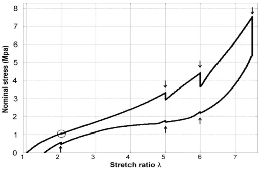
• Cyclic test à It is composed of four sets of three cycles, with four increasing

maximum stretch ratios: λ1= 2, λ2= 5, λ3= 6 and λ4= 7.5, as shown in Figure 1(a).

λ1 was chosen inferior to the crystallization stretch ratio λc, λ2 was close to λc and

finally λ3 and λ4 were superior to λc. The tests were carried out at two constant

loading rates, ±100 mm/min and ±300 mm/min, i.e. at nominal strain rates of ±0.13 s-1 and ±0.5 s-1, respectively.

• Relaxation test 1 à This test consists of a single mechanical load under imposed

displacement at 300 mm/min up to λ= 6, followed by a pause of 8 min (see Figure 1(b)). Here, the fixed value of λ was chosen higher than λc in order to induce stress

8 • Relaxation test 2 à This consists of one mechanical cycle at ±300 mm/min,

including pauses of 30 s at the four previously mentioned stretch ratios, during loading and unloading, as shown in Figure 1(c).

These tests are usually applied for the mechanical characterization of rubber, in order to investigate stress softening, i.e. the Mullins effect [25], loading rate effects, i.e. viscosity effects, crystallization phenomena and cyclic damage.

3.3. Temperature measurement and post-processing

Temperature measurements were performed with a Cedip Jade III-MWIR: see Part 1 for the details [22]. Temperature variations were measured at 147 Hz in a small square zone of 5px X 5px located at the centre of the specimen. A movement compensation technique was used to track this small zone during the test (see [22]).

From a post-processing point of view, the heat sources are obtained from the temperature variations by using the left-hand part of equation (5). The temporal derivate is obtained by finite differences. In practice, temporal filtering was used in order to have a better resolution of the source measurement. Of course, this filtering slightly penalized the temporal resolution of the heat source measurement: for the present study, the minimum duration between two independent values is equal to 0.08s (compared with the temporal resolution of the temperature measurement, which is equal to 1/147 = 0.0068 s).

3.4. Preliminary test to identify τ

The time constant τ involved in the heat diffusion equation (see equation (5)) was experimentally determined. According to equation (3), it depends on:

9 • the material, through the term

!"

• the thickness e à In fact, in current configuration the influence of the thickness

can be seen as the influence of the stretch ratio λ. Indeed, the higher the stretch ratio, the lower the thickness;

• the heat exchange conditions with the environment à For the present 0D approach, the exchanges with the outside environment involve the ambient air as well as the jaws of the testing machine. As the tests are quasi-static (low velocity of the material points), it was considered that the variations in the convection conditions with the ambient air were negligible.

As a result, the function τ (λ) was identified. In practice, ten stretch ratio values ranging from 1 to 7 were used. It is worth noting that the identification must be performed in the same configuration as the mechanical tests (same specimen geometry tightened in the jaws of the testing machine used). The following procedure was used for each case. The specimen was first stretched in the machine. It was then heated by contact with a ‘hot’ piece for a few seconds in order to generate as homogeneous a temperature field as possible. The temperature measurement by IR thermography was performed during the natural return to room temperature. The measurement actually started one minute later, in order to ensure a better homogeneity of the temperature in the specimen.

As an example, Figure 2(a) presents a natural return to ambient temperature at stretch ratio λ=2.15. Solving equation (5) with no heat source (s=0 for a natural return to ambient temperature) leads to the following temperature evolution:

10 where t is the time and θ0 the initial temperature variation considered for the identification

(for t = t0). The unknown parameter τ is identified by least squares method using equation

(6). The values are identified for 10 different stretch ratios. The results are presented in Figure 2(b). It can be observed that the higher the stretch ratio (thus the smaller the thickness of the specimen), the smaller the value of τ. This is in agreement with equation (3). Finally, the experimental data can be fitted by the following linear regression:

! ! = 40.48 − 3.25  ! (7)

The same tests performed for another similar specimen (same material, same dimensions, and same testing conditions) led to a close relation.

4. Results

As shown in Part 1 [22], temperature is not the most relevant quantity to analyze the thermomechanical response of rubbers. Indeed, the temperature variation depends on the level of adiabaticity of the test i.e on the heat exchanges with the environment of the specimen in 0D. This is the reason why the material behaviour is now analyzed in terms of heat source

versus time or stretch ratio, for the three types of test presented above.

4.1. Cyclic test

This test consists of applying four sets of three uniaxial mechanical cycles, with four increasing maximum stretch ratios.

Figure 3(a) shows the evolution of the stretch ratio over the test duration. Figure 3(b) and Figure 3(c) give the corresponding heat source evolutions for both applied loading rates. In Figure 3(a), time is normalized to be homogeneous with the time scale in Figure 3(b) and Figure 3(c). Some comments can be made concerning these results. First, the heat

11 sources are positive during the loading phases and negative during the unloading phases. Second, a dissymmetry is observed between loading and unloading. Third, the higher the loading rate, the larger the heat sources. It is observed that the sources are proportional to the loading rate.

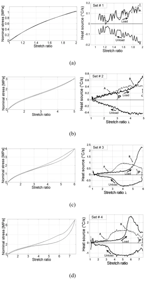
In order to analyze the results more precisely, Figure 4 gives the heat source as a function of the stretch ratio during the first cycle of each set (see Figure 3(a)), for a loading equal to ±300 mm/min. The absolute value of the heat source obtained during unloading is reported in order to compare it with the heat source obtained during loading. The corresponding mechanical response in terms of the stress-strain relationship is also plotted. The following comments can be made:

(i) First cycle of Set #1 (λ1=2), Figure 4(a): During loading, the heat source is positive

and increases with the stretch ratio. This is a major difference with respect to metallic materials, for which the heat sources due to thermoelastic coupling are constant at a fixed strain rate. During unloading, the heat source is negative. Even if the signal-to-noise ratio is too low to enable a good quantitative analysis, some additional comments can be made. It can be seen that the loading-unloading evolution is symmetrical; as a consequence, the total heat produced during loading is equal to the heat absorbed during unloading. In addition, this means that no mechanical dissipation is detected. Indeed, the mechanical dissipation is a positive quantity, and would lead to a positive heat over the whole cycle. This is in a good agreement with the fact that no hysteresis loop is observed in the stress-strain response.

(ii) First cycle of Set #2 (λ2=5), Figure 4(b): The heat source evolutions for loading

12 such a result. During loading, the heat source evolves in a quasi-linear manner until reaching a stretch ratio close to 4. The corresponding curve presents a slope P equal to 0.104 °C/s. This evolution can be explained by entropic coupling. The fact that a dissymmetry is observed if the maximum stretch ratio applied is superior to 4 shows that the heat sources are not caused only by entropic coupling. During unloading, the heat sources are first lower than during loading (between points C and B) and then higher (between points B and A). Nevertheless, the area under the curves during loading and unloading is equal, meaning that no heat is produced due to mechanical dissipation. Consequently, the only explanation for the dissymmetry is the occurrence of crystallization during loading, and a difference in the kinetics of crystallization and crystallite melting (the latter during unloading). This is in a good agreement with studies reported in the literature [2, 23, and 26]. Concerning the stress-strain curve, a hysteresis loop begins to form. It is associated with the crystallization/melting phenomenon, and not with mechanical dissipation.

(iii) First cycle of Set #3 (λ3=6), Figure 4(c): Similarly to the previous set, the heat

source first increases with the same slope P as before, and then strongly increases starting from a stretch ratio close to 4. The loading-unloading dissymmetry of the heat source curves (when crystallization occurs) increases. From a mechanical point of view, the area of the hysteresis loop also increases. As the heat produced is equal to the heat absorbed, it can be deduced that no mechanical dissipation is detected, while the hysteresis loop continues to be observed in terms of the strain-stress relationship.

(iv) First cycle of Set #4 (λ4=7.5), Figure 4(d): The phenomena are similar to those

13 to 6. Indeed, during the loading phase, instead of increasing continuously, the heat source decreases from λ=6. This means that heat continues to be produced (it remains positive), but at a lower rate. This could indicate the fact that this level of stretch ratio tends to approach crystallinity saturation. It should be noted that the hysteresis area in terms of the strain-stress relationship is higher than previously, again with no mechanical dissipation detected.

Figure 5 presents the heat source versus the stretch ratio for the loading phase of the three cycles in each set. It can first be observed that during the first part of the loading (up to point D, see Figure 5 (b), 5(c) and 5(d)), the heat source evolution is the same for the three cycles. This can be related to entropic coupling. Second, from points D to E, the heat source is slightly higher for the first loading than for the next two loading phases. This can be explained by a slight difference in crystallization kinetics between the cycles. When λ exceeds 5.6 - 5.8 (see Figure 5(b) and 5(c)), the heat source is smaller for the first loading than for the next two loading phases. All these observations show that the kinetics of crystallization slightly varies from the first cycle to the others. Nevertheless, no change in the strain-stress relationship is detected.

In summary, mechanical cycles below the stretch ratio at which crystallization begins lead to a symmetric evolution of the heat source between loading and unloading. This accounts for entropic coupling only. Crystallization induces a strong increase in the heat source. The difference in the kinetics of crystallization and crystallite melting leads to a dissymmetry between the loading and unloading curves, and is observed in terms of heat source, but in all cases the heat produced during loading is equal to the heat absorbed during unloading. It should be noted that if no crystallization occurs, no hysteresis loop is observed for the strain-stress relationship. If the stretch ratio is superior to that at which

14 crystallization occurs, a hysteresis loop forms (without any mechanical dissipation). This hysteresis loop is only induced by the difference in the kinetics of crystallization and crystallite melting.

It should be finally noted that the tests performed with a ±100 mm/min loading rate lead to similar results as those performed with a ±300 mm/min loading rate.

4.2. Relaxation test 1

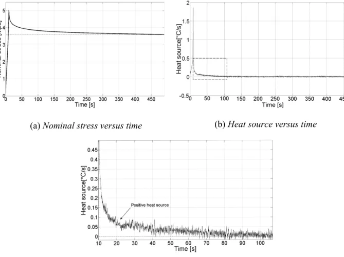
This test consists of applying a single mechanical load under imposed displacement, from λ=1 to λ=6 at a loading rate of ±300 mm/min followed by a pause of 8 min. Figure 6(a) presents the nominal stress versus time. Figure 6(b) presents the corresponding heat source evolution during the test. The following comments can be made.

During the loading phase, the heat source increases. As crystallization begins from λ =4 onwards, approximately, high heat source values (phenomenon discussed in subsection (4.1)) are obtained. At a fixed stretch ratio, the heat source returns progressively to zero. Figure 6(c) shows a magnification of the boxed zone indicated in Figure 6(b). This figure clearly confirms that the heat source does not return to zero instantaneously when the stretch is fixed. It remains positive for about 2 min. It can be noted that, at the same time, the stress continues to decrease. Since the mechanical dissipation due to viscosity has previously been found negligible, the measured heat source is only due to thermomechanical couplings, and more especially to crystallization. It clearly appears that crystallization continues after halting the displacement of the moving grip.

For a better understanding of this result and to discuss the thermomechanical coupling effects, stress evolution versus heat source evolution is presented in Figure 7. The curve obtained can be divided into two parts, [A1A2] and [A2A3], corresponding to different

15 • Between A1 and A2: any change in stress is related to a positive heat source.

• Between A2 and A3: the stress continues to decrease slightly while no heat source is detected. The fact that the stress continues to decrease means that either crystallization slightly continues, or very low viscosity effects come into play. In both cases, they are not detectable with the resolution of the calorimetric technique used.

From these observations, we can conclude that the main part of the stress relaxation amplitude is due to strain-induced crystallization, and possibly also to undetected mechanical dissipation due to viscosity.

4.3. Relaxation test 2

One mechanical cycle is performed under imposed displacement at a ±300 mm/min loading rate. The displacement of the moving grip is halted for 30 s at four stretch ratios, during loading and unloading: λ1= 2, λ2= 5, λ3= 6 and λ4= 7.5. The nominal stress and the

heat source evolution during the test are given in Figures 8(a) and 8(b) respectively. Two typical calorimetric responses are obtained:

• During loading: The heat source is always positive during the successive loading phases. If the stretch ratio is higher than λc=4 approximately, positive heat sources

are detected during the pauses, as explained above. This explains why the temperature continues to increase for a few seconds during stress relaxation (see [22])†_{.No heat source is detected during the pause for stretch ratios lower than λ}

c. • During unloading: The heat source is always negative during the successive

unloading phases, and returns to zero instantaneously when the stretch ratio is maintained constant, apart from the last pause at λ1=2. During the pauses at λ2=5,

† _{It should be noted that the heat source value depends on the temperature rate ! and the heat exchange with the}

16 λ3=6 and λ4=7.5, no heat source is detected from the beginning of the pause: the

heat sources return to zero instantaneously. For the last pause (at λ1=2), the heat

source does not return to zero and remains negative during the whole duration of the pause (30 seconds). This negative heat source, which is incompatible with mechanical dissipation, could be attributed to an additional melting process of the residual crystallites. This is an interesting result that is investigated in the next paragraph.

To study the phenomenon observed during unloading, complementary tests were performed. Compared to relaxation test 2, a new stage was added after the last unloading pause at λ1=2: the specimen was stretched again. Three tests were performed, with three

different relaxation times at λ1=2; [3, 30 and 60 s] (see Figure 9(a)). Each test was

performed three times. The analysis focuses on rigidity at low strains K measured from the strain-stress curve:

• !!! measured after a relaxation time of 3 s (segment [B,B']); • !!"!  measured after a relaxation time of 30 s (segment [C,C']);

• !!"! measured after a relaxation time of 60 s (segment [D,D'];

• !!"!#!$% measured on loading during stretching after the first relaxation time at

λ1=2 (segment [A,A']).

Figure 9(b) shows the nominal stress as a function of the stretch ratio. Here, only the beginning of the curve is considered, and the quantity measured is the slope of the curves. It is observed that material rigidity decreases as a function of relaxation time applied at λ1=2, namely !!!> !!"!>!!"! >!!"!#!$%. This means that the rigidity progressively returns to its lower value !_!"!#!$%.

17 Crystallites act as supplementary reticulation points in the material network and consequently the apparent rigidity increases with crystallite concentration. Then, if the crystals melt progressively at the end of the test, the rigidity also decreases progressively as a function of time and possibly of the number of mechanical cycles (see Figure 9(b)). As a conclusion, crystallite melting could occur not instantaneously during unloading at λ1=2. This could lead to a reconsideration of the physical meaning of melting by

separating, for instance, (i) melting by reducing the size of the crystallites and (ii) the melting of the crystallite germs (more stable thermodynamically).

5. Conclusion

The calorimetric response of unfilled natural rubber has been characterized and interpreted during mechanical cycles and stress relaxation tests. The effects of thermomechanical couplings (entropic coupling and coupling related to crystallization/melting) have been distinguished. Results show that:

• strain-induced crystallization leads to significant heat production whereas the melting of crystallites absorbs the same heat quantity with different kinetics;

• this difference in kinetics explains the hysteresis loop observed with respect to the strain-stress relationship, while no mechanical dissipation is detected during the deformation. Thus, a hysteresis loop in terms of the mechanical response can form without any mechanical dissipation;

• crystallite melting, classically assumed to occur instantaneously compared to crystallite formation, can be time-dependent (this is observed in the present study during unloading for a low stretch ratio). This last remark shows the relevancy of investigating the mechanism of crystallite melting. Further work in this field is currently being envisaged by the authors of this paper.

18

6. Acknowledgements

Authors acknowledge the "Manufacture Française des pneumatiques Michelin" for supporting this study. Authors also thank D. Berghezan, F. Vion-Loisel and E. Munch for the fructuous discussions.

7. Reference List

1. Katz J. Naturw 1925, 4, 169.

2. Toki S, Fujimaki T, Okuyama M. Polymer 2000, 41, 5423–5429.

3. Trabelsi S, Albouy PA, Rault J. Macromolecules 2002, 35, 10054–10061. 4. Legorju-Jago K. Constitutive Models for Rubber V 2007.

5. Feuchter H. Gummi-Ztg 1925, 39, 1167–1168.

6. Ramier J, Chazeau L, Gauthier C, Stelandre L, Guy L, Peuvrel-Disdier E. Journal of Materials Science 2007, 42, 8130–8138.

7. Chrysochoos A, Huon V, Jourdan F, Muracciole, JM, Peyroux R, Wattrisse B. Strain 2010, 46, 117–130.

8. Chrysochoos A, Louche H. Mat Sci Eng A-struct 2001, 307, 15–22.

9. Berthel B, Wattrisse B, Chrysochoos A, Galtier A. Strains 2007, 43, 273–279.

10. Wattrisse B, Chrysochoos A, Muracciole J, Némoz-Gaillard M. Experimental Mechanics 2001, 41, 29–39.

11. Pottier T, Moutrille MP, Le Cam JB, Balandraud X, Grédiac M. Experimental Mechanics 2009, 49, 561–574.

12. Toussaint E, Balandraud X, Le Cam JB, Grédiac M. Polymer Testing 2012, 31, 916– 925.

13. Albouy PA, Guillier G, Petermann D, Vieyres A, Sanseau O, Sotta P. Polymer 2012, 53, 3313–3324.

19 15. Candau N, Chazeau L, Chenal JM, Gauthier C, Ferreira J, Munch E, Rochas C,

Polymer 2012, 53, 2540–2543.

16. Nguyen Q, Germain P, Suquet P. J Appl Sci 1983, 50, 1010–1020. 17. Boccara N. PUF coll. SUP. 1968.

18. Chrysochoos A, Maisonneuve O, Martin G, Caumon H, Chezeau JO. Nuclear Engineering and Design 1989, 114, 323–333.

19. Chrysochoos A, Belmhajoub F. Nuclear Engineering and Design 1992, 44, 55–68. 20. Chrysochoos A, Louche H. Int J Eng Sci 2000, 38, 1759–1788.

21. Chrysochoos A. Analyse du comportement des matériaux par thermographie Infra Rouge. 1995.

22. Samaca Martinez JR, Le Cam JB, Balandraud X, Toussaint E. Submitted for publication in Polymer 2012,

23. Trabelsi S, Albouy PA, Rault J. Macromolecules 2003, 36, 9093–9099. 24. Marchal J. Ph.D. thesis, 2006.

25. Mullins L. Rubber Chemistry and Technology 1948, 21, 281–300. 26. Le Cam JB, Toussaint E. Macromolecules 2008, 41, 7579–7583.18

20

List of Figures

Figure 1: Types of mechanical tests

Figure 2: Identification of the time constant τ characterizing the heat exchanges with the outside of the specimen. Left: example of natural return to ambient temperature, for the specimen stretched at λ = 2.15. Right: values of τ as a function of λ.

Figure 3: Cyclic test. Top: loading applied. Middle: evolution of the heat sources for ±100 mm/min. Bottom: evolution of the heat sources for ±300 mm/min.

Figure 4: Cyclic test at ±300 mm/min: first cycle of each of the four sets. Left: strain-stress curves. Right: heat source versus stretch ratio. The dotted line corresponds to the absolute value of the heat source during the unloading.  

Figure 5: Cyclic test at ±300 mm/min: loading phase of the three cycles of each of the four sets. a) λ1 = 2, b) λ2 = 5, c) λ3 = 6, d) λ4 = 7.5.

Figure 6: Relaxation test 1: nominal stress versus time and corresponding heat sources evolution

Figure 7: Relaxation test 1: stress versus heat source during the stress relaxation stage. Figure 8: Relaxation test 2: heat source versus time.

Figure 9: Complementary tests (final stretching after the relaxation phase upon unloading at λ1=  2)

21

Graphical abstract

22

Figures

(a) Cyclic test

(b) Relaxation test 1

(c) Relaxation test 2

23

Figure 2: Identification of the time constant τ characterizing the heat exchanges

with the outside of the specimen. Left: example of natural return to ambient

temperature, for the specimen stretched at λ = 2.15. Right: values of τ as a

function of λ.

24 (a) cyclic loading.

(b) Heat sources evolutions at ±100 mm/min

(c) Heat sources evolutions at ±300 mm/min

Figure 3: Cyclic test. Top: loading applied. Middle: evolution of the heat sources

for ±100 mm/min. Bottom: evolution of the heat sources for ±300 mm/min.

25 (a)

(b)

(c)

(d)

Figure 4: Cyclic test at ±300 mm/min: first cycle of each of the four sets. Left:

strain-stress curves. Right: heat source versus stretch ratio. The dotted line

26

Figure 5: Cyclic test at ±300 mm/min: loading phase of the three cycles of each

of the four sets. a) λ

= 2, b) λ

= 5, c) λ

= 6, d) λ

= 7.5.

27 (a) Nominal stress versus time

(b) Heat source versus time

(c) Magnification of the heat source evolution during the first 100 seconds of the relaxation

stage

Figure 6: Relaxation test 1: nominal stress versus time and corresponding heat

sources evolution.

28

Figure 7: Relaxation test 1: stress versus heat source during the stress relaxation

stage.

29 (a) Nominal stress versus time

(b) Relaxation test 2: heat source versus time.

Figure 8: Relaxation test 2: Nominal stress versus stretch ratio and heat source

versus time.

30 (a) Three loadings tested, corresponding to three relaxation times at λ1=2 upon unloading

followed by a final stretching.

(b) Strain-stress curves obtained during the final stretching (beginning of the curves). The

curve corresponding to the loading phase [A,A'] is also plotted.

Figure

9

: Complementary tests (final stretching after the relaxation phase upon

unloading at λ

= 2)