Improving the measurement of export instability in the Economic Vulnerability Index: A simple proposal

HAL Id: hal-02128482

https://hal.archives-ouvertes.fr/hal-02128482

Submitted on 14 May 2019

HAL is a multi-disciplinary open access

archive for the deposit and dissemination of sci-entific research documents, whether they are pub-lished or not. The documents may come from teaching and research institutions in France or abroad, or from public or private research centers.

L’archive ouverte pluridisciplinaire HAL, est destinée au dépôt et à la diffusion de documents scientifiques de niveau recherche, publiés ou non, émanant des établissements d’enseignement et de recherche français ou étrangers, des laboratoires publics ou privés.

Improving the measurement of export instability in the

Economic Vulnerability Index: A simple proposal

Sosso Feindouno

To cite this version:

Sosso Feindouno. Improving the measurement of export instability in the Economic Vulnerability Index: A simple proposal. 2019. �hal-02128482�

fondation pour les études et recherches sur le développement international

LA FERDI EST UNE FOND

ATION REC ONNUE D ’UTILITÉ PUBLIQUE . ELLE ME T EN ŒUVRE A VEC L ’IDDRI L ’INITIA TIVE POUR LE DÉ VEL OPPEMENT E

T LA GOUVERNANCE MONDIALE (IDGM).

ELLE C

OORDONNE LE LABEX IDGM+ QUI L

’ASSOCIE A U CERDI E T À L ’IDDRI. CE TTE PUBLIC ATION A BÉNÉFICIÉ D ’UNE AIDE DE L ’É TA T FR ANC AIS GÉRÉE P AR L ’ANR A U TITRE DU PR OGR A MME « INVESTISSEMENT S D ’A VENIR » POR TANT LA RÉFÉRENCE « ANR-10-LABX -14-01 »

poli

cy brief

Introduction

Alongside GNI per capita and the Human Assets Index (HAI),

the Economic Vulnerability Index (EVI) is one of the three criteria

used for the identification of the Least Developed Countries

(LDCs), as used by the UN-CDP (Committee for Development

Policy) at each triennial review of the list of LDCs (see LDC

Handbook, United Nations, 2015). EVI has also been proposed as

a relevant criterion for the allocation of development assistance

(see UN General Assembly resolution on the smooth transition

of graduating LDCs – A/C.2/67/L.5 – and a survey in Guillaumont

2009b; Guillaumont and Wagner, 2013). For the EVI to be still

considered as a useful tool for the identification of LDCs, and

also as an aid allocation criterion, some components (or at least

their calculation) may need to be refined

2

_.

…/…

Sosso Feindouno is a research assistant at Ferdi.

Improving the measurement

of export instability in the

Economic Vulnerability

Index: A simple proposal

Sosso Feindouno 

1



1. Acknowledgments: I want to thank Patrick Guillaumont and Michaël Goujon for their precious comments that greatly improved this document.

2. For example, the share of population in Low Elevation Coastal Zones (LECZ) introduced in 2012 to provide information on countries’ vulnerability to coastal impacts associated with climate change should be revised, with the aim of making it more balanced and equitable (Guillaumont, 2014). The various modifications that can contribute to improving the EVI are also presented and discussed in the document “How to revise EVI?” (forthcoming).

note brève

March 2019

…/… Since 1999, the instability of exports of goods and services has been included as a component in the EVI. The purpose was to reflect the fact that highly variable export earnings cause fluctuations in production, employment, and the availability of foreign exchange, with negative consequences for economic growth and sus-tainable development. Because of the large share of raw materials in production and exports (and often a geographical concentration of export markets), LDCs are characterized by high export instability. This instability constrains their capacity to implement investment programs through its impact on domestic saving, tax revenue, and import capacity. Moreover, instability in export earnings increases uncertainty with a negative impact on private investment. It also has detrimental social consequences, lowering the impact of the average rate of growth on poverty reduction (Guillaumont, 2009b).

The UN-CDP considers the instability of exports of goods and services to be one of the most important components of the EVI3_{. Thus, the way in which this}

component is calculated deserves particular attention. Since the EVI is a criterion for aid allocation, any improvement in the calculation of its components (especially, as here, export instability) would be commendable and could have direct repercus-sions on people through LDC identification and aid allocation.

Measurement of Instability

In the literature, a variety of measures of instability have been proposed, each one with its particular strengths and weaknesses (see a recent review in Cariolle and Goujon, 2015). The coefficient of variation is the “natural” and the simplest measure of export instability. But in most cases, instability is calculated as the mean squared deviation from an estimated long-term trend, either linear or exponential (e.g. Massel, 1970). This approach of measuring instability around a trend may depend on the choice of the form of the trend. The choice of an appropriate form of the trend is thus a crucial element of the construction of a suitable index of export earnings instability.

Modelling trends in time series has long been of interest in the literature4_.

The exercise of identifying the appropriate trend remains a theoretical challenge, as noted by Phillips (2005) “no one understands trends, but everyone sees them in the data”. Trends fall into two categories depending on whether the trends are stochastic or deterministic. A deterministic trend, which is generally modelled by a straight line over time, may produce fluctuations at each point generated by a

3. Instability of export of goods and services has a high weight in the EVI (1/4 of the EVI and 1/2 of the shock sub-index).

4. Phillips (2005) provides an overview covering the development, challenges, and some future direc-tions of trend modelling in time series. White and Granger (2011) offer working definidirec-tions of various kinds of trends and invite more discussion on better methods of estimating trends.

2

Policy brief n°189

S

osso F

purely stochastic mechanism5_{. In that respect, deterministic and stochastic trends}

are often indistinguishable, in particular when only a relatively short portion of the series is available. This is why, since the introduction of the instability of goods and services in the EVI, the trend is assumed to have both a deterministic and a stochastic component. This method used at CERDI/FERDI for a number of years is called a “mixed trend” regression, as shown in the following equation:

log y

_t

= α + β log y

_t-1

+ γT + ε

_t

(1) Where,

y

_t is the value of exports of goods and services at constant US dollars in year t;

T

is the time variable;

ε

_t is the error term in year t;

α, β and γ are the regression coefficients.

Equation (1) is estimated separately for each country, using standard ordinary least squares (OLS) over a specific time period. Associated with the choice of the type of trend, choosing an appropriate time period is also of paramount importance. The length of the period retained by the UN-CDP has changed over time (15 years for the 2006 and 2009 reviews, 20 years for the 2012 review, and 21 years for the 2015 and 2018 reviews). A trend calculated over 15, 20 (or 21) years seems to be a reasonable basis (as discussed by Cariolle and Goujon, 2015).

In this document, we question the linearity of the deterministic part of the trend, which may be too restrictive to capture asymmetries and observed non-linear dynamics. When the time period is longer, there is a risk that the deterministic com-ponent of the trend is no longer linear. Thus, both for capturing a possible change in the deterministic trend and avoiding a high impact of the chosen time period, we propose to fit a quadratic trend to the model using the following equation:

log y

_t

= α + β log y

_t-1

+ γT + θT

2

_{+ ε}

t

(2)

Is the current fit of the trend valid for all countries?

Because developing countries are heterogeneous, applying a single predefined model to all countries could have its limits, since a model may be more relevant for some countries than others. On the other hand, making the instability indicator comparable across countries requires the use of an identical de-trending method, which amounts to applying the mixed trend to all countries. This is why we first

5. Shocks may permanently affect the series and lead to a purely stochastic series. The stochastic trend is one that can change in each run due to the random nature of the process.

3

Policy brief n°189

S

osso F

test whether the mixed trend method is suitable for all the countries in our sample. The trend aspects of each country can be assessed by a measure called the Mean Absolute Scaled Error (MASE)6_{, which is calculated by:}

MASE = mean(|q

_t

|)

; where

q

_t is defined as

q

_t

=

With

Y

_t the value of exports of goods and services at constant US dollars in year

t

,

Ŷ

_t the predicted value of exports of goods and services in year

t

obtained from model (1),

T

the forecasting horizon.

The bigger the MASE, the worse the fit of the trend to the data. This measure is easily interpretable. Values of MASE greater than one indicate that the trend fit-ting method does not provide a good enough fit to the exports series for which it is estimated. Overall, if we take the sample of 145 developing countries (the same sample as the UN-CDP), the mixed trend method is a good estimate of the trend. But for 11 countries7_{, a MASE greater than one reveals that the mixed trend is not}

a good enough form of the trend.

So, considering the MASE criterion after adding a quadratic trend, the MASE is greater than one only for 7 countries (Palau, Tuvalu, Papua New Guinea, Gambia, Central African Republic, Comoros and Timor-Leste), they have a poorly estimated trend. These countries, except the Central African Republic, are already in the list of the 11 countries mentioned in the case of the use of a simple mixed trend. For the vast majority of countries, adding a quadratic trend to the simple mixed trend lowers the MASE values.

To confirm this outcome, and to supplement the MASE criterion, another criterion called the Mean Absolute Percentage Error (MAPE) is used to select a better fitted model for trends. The MAPE is one of the most popular measures in the forecasting literature (Ahlburg, 1995; Hyndman and Koehler, 2006; Wilson, 2007); it is simple to calculate and easy to understand. But MAPE has a significant drawback: it is not a robust measure in the presence of outliers, and it produces infinite or undefined values when the observed values are zero or close to zero. It can be defined as:

MASE =

|PE

_t

|

; where

PE

_t

= 100* (Y

_t

- Ŷ

_t

) / Y

_t

6. When series include outliers or extreme values, it is advisable to apply scaled measures such as MASE. However, to use the MASE, the time period should be large enough (21 years in our case). 7. These countries are: Tuvalu, Palau, Timor-Leste, Papua New-Guinea, Libya, Comoros, Bhutan, Nepal,

Democratic People’s Republic of Korea, South Sudan, and Gambia.

4

Policy brief n°189

S

osso F

The countries for which a mixed trend leads to a better fit of the trend are presented in Table 1. The countries are arranged in order of importance of the difference be-tween the MASE (or MAPE) of the mixed trend and that of the augmented mixed trend. According to both criteria, the list of countries is the same, except for Somalia for which the MAPE is the same for the two estimated trends. The mixed trend is better suited to estimating the trend of countries such as Palau, Marshall Islands, Central African Republic, and Gambia. With the exception of the countries listed in Table 1, it is clear that for the bulk of developing countries, the addition of the quadratic term contributes to a better estimate of the trend and consequently to a better calculation of instabilities.

Table 1. Countries which best fit mixed trend

MASE criterion MAPE criterion

Country ISO MT MT+QT Country ISO MT MT+QT

Palau PLW 1.092 1.282 Palau PLW 1.098 1.270

Marshall Islands MHL 0.714 0.816 Gambia GMB 2.242 2.318

Central African Republic CAF 0.970 1.017 Marshall Islands MHL 0.257 0.293

Gambia GMB 1.001 1.048 Central African Republic CAF 0.484 0.507

Algeria DZA 0.774 0.792 Chad TCD 0.852 0.867

Ghana GHA 0.704 0.720 Ghana GHA 0.544 0.555

Iran IRN 0.898 0.912 Iran IRN 0.260 0.264

Barbados BRB 0.986 0.998 Turkey TUR 0.157 0.161

Turkey TUR 0.544 0.556 Barbados BRB 0.256 0.259

Chad TCD 0.887 0.897 Nigeria NGA 0.625 0.628

Philippines PHL 0.637 0.644 Mauritania MRT 0.336 0.339

Mauritania MRT 0.765 0.772 Philippines PHL 0.228 0.231

Papua New Guinea PNG 1.072 1.078 Algeria DZA 0.123 0.126

Mexico MEX 0.502 0.507 Lao PDR LAO 0.470 0.472

Solomon Islands SLB 0.751 0.756 Solomon Islands SLB 0.591 0.593

Lao PDR LAO 0.847 0.852 Lesotho LSO 0.420 0.422

Lesotho LSO 0.707 0.711 Mexico MEX 0.117 0.119

Nigeria NGA 0.804 0.808 Papua New Guinea PNG 0.328 0.329

Morocco MAR 0.379 0.381 Oman OMN 0.277 0.277

Somalia SOM 0.419 0.422 Morocco MAR 0.104 0.105

Oman OMN 0.855 0.858      

Note: MT=Mixed Trend; QT=Quadratic Trend; the lower the MASE or MAPE score, the better is the fit.

5

Policy brief n°189

S

osso F

In addition to the MASE and MAPE criteria, the selection of the appropriate model for each country can be done in several ways, the best known of which is

R

2. The greater the

R

2, the better the fit of the trend to the data. Since the models from equations (1) and (2) are nested,

R

2 cannot decrease when we add a quadratic trend; the fit will be equal or better. This is why we do not use the criterion, although the use of adjusted R-squared can help to partially overcome this difficulty. The choice of

R

2 criterion would have made sense, if for example the question was whether the deterministic or stochastic trend is the most appropriate for a given country.

What happens when we add a quadratic trend?

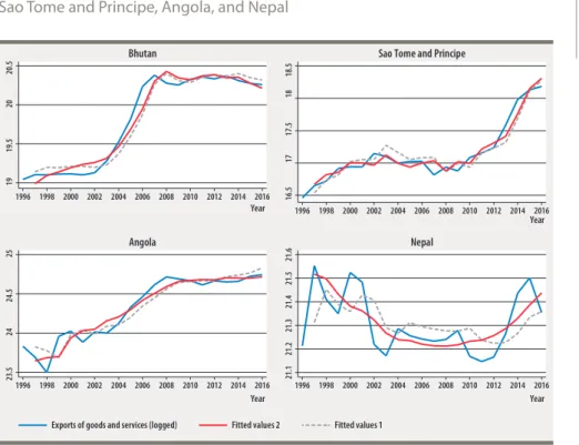
The trend of export earnings is clearly non-linear, and an infinite number of func-tions enables dealing with this non-linearity. It requires significant effort to deter-mine the function that provides the optimal fit for the value of exports of goods and services. In our case, we show how a simple addition of a quadratic trend con-tributes to a better calculation of export instabilities in the EVI. It makes it possible to highlight and better capture possible changes in trend compared to a mixed trend where the deterministic component is linear. It is an augmented mixed trend. Time series plots of export earnings are given for 4 LDCs: Bhutan, Sao Tome and Principe, Angola, and Nepal. These are among the countries for which the addition of a quadratic trend has the largest influence on the country’s instability calculation by the MASE criterion, since for the 4 countries the trend in the series of exports is far from linear. For each of these countries, fitted values of exports are generated from the mixed trend (Fitted values 1, following equation 1) and the addition of quadratic trend to mixed trend (Fitted values 2, following equation 2).

6

Policy brief n°189

S

osso F

Figure 1. Exports of goods and services, fitted values for Bhutan, Sao Tome and Principe, Angola, and Nepal

What impact on the values of instability and ranks?

A quadratic trend is likely to capture the nonlinearity of a deterministic trend. The model might not be the best for all countries, but it is clearly better than the current model used for the EVI calculation by the UN-CDP. So, applying the new model to the computation of the instability of export of goods and services would lead to an improvement in the results of the EVI. For LDCs, we have tentatively calculated the export instability with this new formula for the trend. In Table 2, we compare the country ranks with those obtained by using the mixed trend method (for two different time periods). Let us consider “instability 1” the instability obtained from the UN-CDP and “instability 2” the instability obtained from the new formula based on a trend form that includes a quadratic trend. The rank difference is computed as a positive difference between countries that rank relatively better because of a lower score in instability 2 than in instability 1. If we use a 21-year period to calculate the trend and instability (as used in the 2018’s CDP review), the countries which have the biggest positive rank changes are Bhutan (+9), Sao Tome and Principe (+6), and Malawi (+5); the biggest negative rank changes are for Lao PDR and Mauritania (-6). The results are more sensitive when the calculation period is 15 years: Sao Tome and Principe, Ethiopia and Guinea-Bissau rise 10, 8 and 7 ranks respectively, while

7

Policy brief n°189

S

osso F

Zambia and Solomon Islands fall 5 ranks, and Rwanda and Guinea 4 ranks. At the bottom of the ranks column, we give the average of the absolute differences of rank between the two measures of instability. This average is lower for the 21 year period than for the 15 year period.

But what matters is the impact of the new formula on countries’ instability indices and consequently on their levels of EVI. Table 2 provides the results by country and the average value of absolute differences between various measures of instability. If we use a 15 year time period, the instability indices (or scores) of all countries fall, except Zambia and Liberia. Timor-Leste is by far the country with the largest decline (-22.7 points), followed by Guinea-Bissau (-4.9points) and Sao Tome and Principe (-4.8 points). Also, when a 21 year time period is used, only the instability scores of Madagascar, Guinea, Myanmar and Togo do not fall. The larg-est decreases are observed in Sudan (-14.7 points), Timor-Llarg-este (-14.1 points) and Eritrea (-9.5 points).

Table 2 highlights the sensitivity of instability to the length of the calculation period. The longer the period, the higher the average absolute value of differences between instability 2 and instability 1. Finally, for both types of instability, we ex-amine the impact of the length of the calculation period (15 years vs 21 years). From the average absolute value of differences, we can say that the impact of the period increases when the instability is calculated with the addition of a quadratic trend.

Conclusion

Given the importance of the instability of export of goods and services in the EVI, any significant error in scores and ranks may have an impact on the EVI, and in turn on people through resource allocation. That is why special attention should be devoted to measuring the instability of exports of goods and services in the EVI. The UN-CDP calculates the instability of export of goods and services by estimating the trend of export earnings using a mixed trend linear regression. The standard deviation of the differences between trend and observed values is then taken as a measure of instability. The determination of the appropriate form of trend to calculate instability remains a big challenge. In this brief, we show that the calcula-tion of the index of export earnings instability could be improved by estimating an augmented mixed trend. This consists of adding a quadratic trend, which would help to capture nonlinearity in the deterministic trend. As the UN-CDP calculates instability over a long period of time, this method would better capture possible changes in the deterministic trend which are more likely to occur when the time period is longer. This proposal results in significant ranking changes of the index for some countries, as shown in Table 2.

8

Policy brief n°189

S

osso F

Table 2. Instability of exports of goods and services of LDCs: Current CDP version and revised version for different time periods: 15 and 21 year periods

Country ISO 15 years [A] Rank. diff. Value[A2] – Value[A1] 21 years [B] Rank. diff. Value[B2] – Value[B1] Value[B1] – Value[A1] Value[B2] – Value[A2]

Instability1 Instability2 Instability1 Instability2

Value[A1] Rank Value[A2] Rank Value[B1] Rank Value[B2] Rank

Afghanistan AFG 19.57 9 17.34 9 0 -2.22 20.86 10 17.10 10 0 -3.76 1.29 -0.24

Angola AGO 6.29 37 6.00 36 -1 -0.29 12.63 27 12.00 24 -3 -0.63 6.35 6.00

Burundi BDI 16.51 13 12.23 14 1 -4.29 17.19 11 16.87 11 0 -0.31 0.68 4.65

Benin BEN 10.40 26 9.57 26 0 -0.83 10.37 35 9.18 35 0 -1.19 -0.03 -0.39

Burkina Faso BFA 10.00 28 9.27 28 0 -0.73 13.02 23 12.77 21 -2 -0.25 3.02 3.50

Bangladesh BGD 8.03 33 5.47 39 6 -2.56 7.02 42 6.44 42 0 -0.58 -1.01 0.97 Bhutan BTN 11.88 22 10.22 21 -1 -1.66 13.53 22 10.66 31 9 -2.88 1.65 0.43 Central African Republic CAF 10.40 25 9.76 25 0 -0.63 11.41 32 11.21 28 -4 -0.20 1.01 1.44 DR Congo COD 11.27 24 10.09 22 -2 -1.18 15.44 16 14.96 15 -1 -0.48 4.17 4.87 Comoros COM 16.86 11 16.84 10 -1 -0.02 15.89 15 15.57 14 -1 -0.32 -0.97 -1.27 Djibouti DJI 4.57 43 4.57 42 -1 -0.01 5.67 44 5.58 44 0 -0.09 1.10 1.01 Eritrea ERI 41.13 3 40.73 2 -1 -0.40 46.09 3 36.56 3 0 -9.53 4.96 -4.17 Ethiopia ETH 11.52 23 8.62 31 8 -2.89 12.69 26 10.70 30 4 -1.99 1.17 2.08 Guinea GIN 15.51 15 14.90 11 -4 -0.62 14.24 19 14.35 18 -1 +0.10 -1.27 -0.55 Gambia GMB 57.41 2 56.08 1 -1 -1.33 51.22 2 47.65 2 0 -3.57 -6.19 -8.44 Guinea-Bissau GNB 16.72 12 11.79 19 7 -4.93 22.61 9 20.03 9 0 -2.58 5.89 8.24 Equatorial Guinea GNQ 8.84 31 7.19 33 2 -1.65 13.01 24 11.34 26 2 -1.67 4.17 4.15 Haiti HTI 5.58 41 5.02 41 0 -0.56 6.12 43 5.97 43 0 -0.15 0.54 0.95 Cambodia KHM 6.03 39 5.62 37 -2 -0.41 10.37 36 7.24 40 4 -3.13 4.34 1.62 Kiribati KIR 11.98 20 11.84 18 -2 -0.14 16.76 13 16.67 12 -1 -0.09 4.78 4.83 Lao PDR LAO 9.75 30 9.10 29 -1 -0.65 12.53 28 12.47 22 -6 -0.07 2.78 3.36 Liberia LBR 34.27 5 35.04 5 0 +0.76 32.11 6 31.54 4 -2 -0.57 -2.17 -3.49 Lesotho LSO 6.14 38 6.13 35 -3 -0.01 10.84 33 10.12 33 0 -0.71 4.70 3.99 Madagascar MDG 15.52 14 14.43 13 -1 -1.10 14.61 17 14.80 16 -1 +0.19 -0.92 0.37 Mali MLI 8.69 32 8.69 30 -2 -0.00 10.79 34 10.62 32 -2 -0.17 2.10 1.92 Myanmar MMR 13.03 19 11.97 17 -2 -1.07 13.81 20 13.81 20 0 +0.01 0.77 1.85 Mozambique MOZ 4.82 42 3.61 43 1 -1.21 9.91 37 8.63 37 0 -1.28 5.09 5.02 Mauritania MRT 13.37 18 12.10 15 -3 -1.27 12.34 29 12.25 23 -6 -0.09 -1.03 0.15 Malawi MWI 18.25 10 14.73 12 2 -3.52 17.06 12 14.38 17 5 -2.68 -1.19 -0.35 Niger NER 7.91 34 5.31 40 6 -2.60 8.81 38 8.75 36 -2 -0.05 0.90 3.44 9

Country ISO 15 years [A] Rank. diff. Value[A2] – Value[A1] 21 years [B] Rank. diff. Value[B2] – Value[B1] Value[B1] – Value[A1] Value[B2] – Value[A2]

Instability1 Instability2 Instability1 Instability2

Value[A1] Rank Value[A2] Rank Value[B1] Rank Value[B2] Rank

Sudan SDN 24.08 8 23.92 8 0 -0.16 40.73 4 25.98 7 3 -14.75 16.65 2.06

Senegal SEN 3.04 45 2.33 45 0 -0.71 4.04 45 3.71 45 0 -0.33 1.00 1.38

Solomon

Islands SLB 9.90 29 9.79 24 -5 -0.10 14.52 18 13.94 19 1 -0.58 4.62 4.14

Sierra Leone SLE 35.24 4 35.08 4 0 -0.16 30.28 8 30.14 5 -3 -0.14 -4.96 -4.94

Somalia SOM 1.31 46 1.12 46 0 -0.19 2.04 46 1.88 46 0 -0.16 0.73 0.75

Sao Tome and

Principe STP 14.26 17 9.45 27 10 -4.80 13.78 21 11.28 27 6 -2.51 -0.47 1.82 Chad TCD 27.02 7 25.84 7 0 -1.18 30.35 7 25.83 8 1 -4.53 3.33 -0.02 Togo TGO 7.49 35 7.47 32 -3 -0.02 7.93 39 7.93 38 -1 0.00 0.44 0.46 Timor-Leste TLS 61.04 1 38.36 3 2 -22.68 74.33 1 60.26 1 0 -14.07 13.29 21.90 Tanzania TZA 5.70 40 5.51 38 -2 -0.19 7.46 40 6.68 41 1 -0.78 1.76 1.17 Uganda UGA 15.47 16 10.94 20 4 -4.53 16.54 14 16.32 13 -1 -0.22 1.07 5.38 Vanuatu VUT 4.55 44 3.41 44 0 -1.13 7.42 41 7.41 39 -2 -0.01 2.87 4.00 Yemen YEM 31.00 6 29.11 6 0 -1.89 32.14 5 29.43 6 1 -2.71 1.15 0.33 Zambia ZMB 11.96 21 11.98 16 -5 +0.02 12.81 25 11.71 25 0 -1.10 0.84 -0.28 Average absolute value of the instability measures and their differences

15.26 13.60 2.13 1.69 17.31 15.52 1.73 1.81 2.93 2.97

Note: Instability 1 is the instability calculated by the CDP method (deterministic trend and a stochastic modelled with a one year lag variable).

Instability 2 is the instability calculated by a regression on the trend, quadratic trend and one year lag variable.

References

•

Ahlburg, D. A. (1995). Simple versus complex models: Evaluation, accuracy, and combining. Mathematical Population Studies, 5(3), 281-290.

•

Cariolle, J. & Goujon, M. (2015). Measuring macroeconomic instability: A criti-cal survey illustrated with exports series. Journal of economic surveys, 29(1), 1-26.

•

Cariolle, J., Goujon, M. & Guillaumont, P. (2016). Has structural economic vulnerability decreased in Least Developed Countries? Lessons drawn from ret-rospective indices. The Journal of Development Studies, 52(5), 591-606.

•

Feindouno, S. & Goujon, M. (2016). The retrospective economic vulnerability

index, 2015 update, Ferdi Working Paper 147, March 2016.

•

Guillaumont. P. (2009b). “An Economic Vulnerability Index: Its Design and Use for International Development Policy”. Oxford Development Studies. 37 (3). 193-228

•

Guillaumont, P. (2013), Measuring structural vulnerability to allocate develop-ment assistance and adaptation resources, FERDI Working Paper 68, March 2013, revised version September 2013.

•

Guillaumont. P. (2014). “A necessary small revision to the EVI to make it more balanced and equitable”. FERDI. policy brief 98. July 2014.

•

Guillaumont, P. (2017) Vulnerability and Resilience: A Conceptual Framework applied to Three Asian Poor Countries — Bhutan, Maldives and Nepal, Asian Development Bank, South Asia Working Paper Series, No 53, October, 76 p.

•

Massell. B. F. (1970). “Export instability and economic structure.” American

Economic Review. vol. 60. n°.4. pp. 618-30.

•

Phillips, P. C. (2005). Challenges of trending time series economet-rics. Mathematics and Computers in Simulation, 68(5-6), 401-416.

•

United Nations (2018). Handbook on the Least Developed Country Category:

Inclusion. Graduation and Special Support Measures. United Nations Committee for

Policy Development and Department of Economic and Social Affairs. 3rd edition.

•

White, H. & Granger, C. (2011). Consideration of trends in time series. Journal of Time Series Econometrics 3, 1-40.

•

Hyndman, R. J., & Koehler, A. B. (2006). Another look at measures of forecast accuracy. International journal of forecasting, 22(4), 679-688.

•

Wilson, T. (2007). The forecast accuracy of Australian Bureau of Statistics national population projections. Journal of Population Research, 24(1), 91-117.

11

Policy brief n°189

S

osso F

not

e brève

Créée en 2003, la Fondation pour les études et recherches

sur le développement international vise à favoriser la

compréhension du développement économique international

et des politiques qui l’influencent.

Contact

www.ferdi.fr

contact@ferdi.fr

+33 (0)4 73 17 75 30

n° ISSN : 2275-5055

policy brie

f

March 2019

189