Modelling Variability in the Leader Algorithm Family: A Testable Model and Implementation

(1)

https://doi.org/10.4224/5763719

READ THESE TERMS AND CONDITIONS CAREFULLY BEFORE USING THIS WEBSITE. https://nrc-publications.canada.ca/eng/copyright

Vous avez des questions? Nous pouvons vous aider. Pour communiquer directement avec un auteur, consultez la première page de la revue dans laquelle son article a été publié afin de trouver ses coordonnées. Si vous n’arrivez pas à les repérer, communiquez avec nous à PublicationsArchive-ArchivesPublications@nrc-cnrc.gc.ca.

Questions? Contact the NRC Publications Archive team at

PublicationsArchive-ArchivesPublications@nrc-cnrc.gc.ca. If you wish to email the authors directly, please see the first page of the publication for their contact information.

NRC Publications Archive

Archives des publications du CNRC

For the publisher’s version, please access the DOI link below./ Pour consulter la version de l’éditeur, utilisez le lien DOI ci-dessous.

Access and use of this website and the material on it are subject to the Terms and Conditions set forth at

Modelling Variability in the Leader Algorithm Family: A Testable Model

and Implementation

Barton, Alan

https://publications-cnrc.canada.ca/fra/droits

L’accès à ce site Web et l’utilisation de son contenu sont assujettis aux conditions présentées dans le site LISEZ CES CONDITIONS ATTENTIVEMENT AVANT D’UTILISER CE SITE WEB.

NRC Publications Record / Notice d'Archives des publications de CNRC: https://nrc-publications.canada.ca/eng/view/object/?id=3bae5e69-bd07-4f3e-8898-366508ad07ba https://publications-cnrc.canada.ca/fra/voir/objet/?id=3bae5e69-bd07-4f3e-8898-366508ad07ba

(2)

National Research Council Canada Institute for Information Technology Conseil national de recherches Canada Institut de technologie de l'information

Modelling Variability in the Leader Algorithm

Family: A Testable Model and Implementation *

Barton, A.

December 2004

* published as NRC/ERB-1119. 54 Pages. December 20, 2004. NRC 47429.

National Research Council of Canada

Permission is granted to quote short excerpts and to reproduce figures and tables from this report, provided that the source of such material is fully acknowledged.

(3)

Modelling Variability in the Leader Algorithm Family:

A Testable Model and Implementation

Alan J. Barton

Integrated Reasoning Group Institute for Information Technology

National Research Council Canada Ottawa, Canada, K1A 0R6 alan.barton@nrc-cnrc.gc.ca

(4)

Abstract

This final project report1 is a Type I: Modelling variability into a testable model project. The main themes of the course revolve around the concepts of variability (in this project variability is associated with the variation of an algorithm in time i.e. evolutionary vari-ability and with varivari-ability in definitions of concepts), tracevari-ability and verification. Hence these concepts form the core focus of this project, with more emphasis being placed on the creation of a traceable, testable domain model. In particular, two questions posed during the offering of this course are: i) “Can tests be used to document how family members are different?”, and ii) “How can features and their dependencies be properly documented?”

1_{Submitted to Professor Jean-Pierre Corriveau in partial fulfillment of the requirements of the computer}

science course COMP 5104 - Object Oriented Software Engineering and to the National Research Council as an internal technical report.

(5)

Modelling Variability in the Leader Algorithm Family Bibliography 42 8 Appendix 44 8.1 Test case 1 . . . 44 8.2 Test case 2 . . . 45 8.3 Test case 3 . . . 46 8.4 Test case 4 . . . 46 8.5 Test case 5 . . . 47 8.6 Test case 6 . . . 48 8.7 Test case 7 . . . 49 8.8 Test case 8 . . . 49 8.9 Test case 9 . . . 50 8.10 Test case 10 . . . 51 8.11 Test case 11 . . . 52 8.12 Test case 12 . . . 52 Index 54

(7)

List of Figures

2.1 Relationship of Project Goals to Project Work Products . . . 9

4.1 Conceptualization of Clustering Process . . . 15

4.2 Use Case (UC) for Leader Algorithm Family . . . 16

4.3 Use Case Map (UCM) for Leader Algorithm Family . . . 17

5.1 Abstract representation of a data matrix in primary memory. . . 33

5.2 One variant of sorting incomplete data objects (X = CSI) . . . 34

5.3 O(2n) range sort for incomplete data objects . . . 34

5.4 Variants of indexing schemes . . . 34

(8)

List of Tables

3.1 Family Members . . . 12

4.1 Feature and Feature Value Identifiers . . . 18

4.2 Parameter and Parameter Value Identifiers . . . 19

4.3 Interaction Codes . . . 20

4.4 Member–Feature Relationships. . . 20

5.1 Three possible modified distances ([19]p.1947) . . . 31

5.2 Mapping of abstract preprocessing component to concrete components . . . 32

5.3 Mapping of abstract algorithm component to concrete components . . . 32

5.4 Mapping of abstract postprocessing component to concrete components . . 32

(9)

List of Algorithms

1 Hartigan’s Leader Algorithm (Translation) . . . 13

(10)

Nomenclature

Td A dissimilarity (or distance) threshold

Ts A similarity threshold (See §5.1)

X The original (possibly huge) data set

O(g(n)) = {f (n) : ∃c, n0> 0, s.t. 0 ≤ f (n) ≤ c · g(n), ∀n ≥ n0}

(11)

Chapter 1 Introduction

The Method of Multiple Working Hypotheses – T.C. Chamberlin 18901

T

here are many things in this world that are not certainly known or understood by humans. It is best, therefore, to consider multiple competing (variable) hypotheses2 in order to attempt to understand3 _{the inherent complexity in the world around us and}

to be able to disseminate that knowledge (communicate these hypothesis for others). In particular, it is assumed that the larger the variability in the set of hypotheses under consideration, then the higher the likelihood one of them may very accurately describe the complex world.

In the field of software engineering, one software system is usually built for a particular domain in order to help domain experts (users) understand some aspects of their domain. It has been proposed that it might be better to consider all possible systems (a family) that could be built for a particular domain, instead of only one system at a time (classical approach). This concept, called system family engineering, attempts to more explicitly ex-plicate (“clearly explain” would be another variation of this word combination) the tradeoffs between design (implementation) alternatives, individually known as family members.

Further, the classical testing approach focuses on the consideration of one software system at a time (called the system under test). However, a competing approach considers testing from the point of view of a whole family of software systems and at the much more abstract and user centered domain modelling level. This approach leads to objective tests that are directly derived from a model of the whole family of systems.

1_{Thomas C. Chamberlin (1843-1928) wrote about the method of multiple working hypotheses in [4].} 2_{Multiple hypotheses could also be called a family of hypotheses.}

3_{Objectivity is chosen over subjectivity (or intuition) whenever possible in this project.}

(12)

Chapter 2 Project

T

he family of algorithms that will be investigated, as the domain under consideration, are related to clustering data. That is, the Leader Algorithm originally proposed by John A. Hartigan in [10] along with variants that Dr. Julio Vald´es proposed will be investigated. A fortran implementation of the original algorithm is available in [10] and a variant was made available by Dr. Julio Vald´es in ANSI C. This project proposal is a research topic in its domain, as well as being a research topic for the purposes of the course.

Definition 1 (Program Family) In 1976 David L. Parnas [12] wrote that:

We consider a set of programs to constitute a family, whenever it is worthwhile to study pro-grams from the set by first studying the common properties of the set and then determining the special properties of the individual family members.

2.1 Project Conceptualization

The project aims to investigate how abstract models of a domain (in this case Testable Feature Contracts) can lead, via a structured and systematic approach to abstract tests. See Fig-2.1 for a visual representation of the project goals (i.e. i) Testable Domain Models and ii) Derived Tests) and their relationship to the project work products (e.g. Feature Contracts are intended to be a testable domain model because, for example, dynamic tests can be derived from them in a systematic way).

2.2 Project Domain Scope

This project will require the implementation of Hartigan’s Leader Algorithm and variants, in the American National Standards Institute (ANSI) C Standard, which has been adopted as an international standard (ISO/IEC 9899:1990) [16]. Even though this course is a course in object oriented software engineering, the focus is on the essence of object orientation (as revealed during one lecture by Professor Corriveau when questioned by the author), and so the implementation language of ANSI C was deemed to be appropriate.

The aforementioned implementation work, and the building of testable models lie within the scope of this project. However, it is recognized that the implementation work will not be for credit towards the course objectives, but, none-the-less, it is considered as a possibly useful contribution for the ongoing research in the Integrated Reasoning Group of the Institute for Information Technology of the National Research Council Canada.

(13)

Modelling Variability in the Leader Algorithm Family Testable Feature Contracts Static Tests Dynamic Tests Features (and combinations) Domain

Not project focus:

Gui Mockups Sequence Diagrams Activity Diagrams State Diagrams Class Diagrams Implementation (code)* Code Integration* Unit/Regression Testing* Test Cases* Usability Testing

*Included in project work

Use Case (Group of Scenarios)

Use Case Map Testable

Domain Model Derived Tests

Figure 2.1: Relationship of Project Goals to Project Work Products

In addition, it is recognized that there are certainly other clustering algorithms that could be considered. They are, however, variants of a more general, and much larger family, which would involve too much time (than the duration of the course) to investigate and document thoroughly. For example, other clustering algorithms include: i) kmeans, ii) SOM, iii) TaxMap, iv) Hierarchical divisive, v) Hierarchical agglomerative, etc. of which one possible taxonomy (concept hierarchy variant) of these methods is given in ([14] p.201). Only a small subset of the Leader Algorithm Family will be considered. In particular, i) parallel or distributed [2] variants of the leader algorithm will not be considered, as no currently known implementation exists that could be modelled, and ii) at most two distance (no similarity) functions will be implemented, as the investigation of an appropriate function is left to the scientific investigation of the particular data set and its associated application domain properties. That is, the data may come from very many possible domains, but only a simulated data set domain will be considered, as an algorithm variant works the same on any given data set domain; so, considering data domain variants is also outside the scope of this project. In particular, data sets could be i) biological, genetic (cDNA microarray data [20]), or proteomic (mass spectrometry data), or ii) in another domain entirely, such as in astronomy for grouping similar galaxies [17]. Therefore, deriving all possible tests from the domain model for a family member, would require knowing about the data set used, which would require knowing something about the domain. This is completely outside the scope of this project, and so a data set that the author is familiar with will be used. That is, an artificially constructed data set will be used for conformance-directed and fault-directed testing.

Nonfunctional features could be considered in terms of, for example, performance, be-cause the different family members (variants) will potentially have different computational complexity. However, nonfunctional features will not be considered in this project.

(14)

Modelling Variability in the Leader Algorithm Family

2.3 Project Constraints and Coverage

For this project, time was a large constraint, because implementation and then modelling work needed to be performed. Indeed, a large body of material was covered in the course from many sources, of which [3] and [6] are the main references; while no material was directly used from the presented works of [11] and [9]. For example, [8] covers material related to i) Objects and UML, ii) basic concepts of real-time systems and safety-critical systems, iii) rapid object-oriented process for embedded systems, iv) requirements analysis for real-time systems, v) structural and behavioral object analysis, vi) architectural, mech-anistic and detailed design, vii) advanced real-time object modelling including threads and schedulability, dynamic modelling and real-time frameworks.

In addition, the classical papers ([7] and [12]) were obtained and read; in order to understand the original motivations for structured programming and programming families. Template metaprogramming [6] was not used, because, i) it is a C++ specific program-ming language construct and this project has the constraint that it should be ANSI C, ii) if it was used, it may be very difficult to debug the code if it turned out that testing the generated code revealed problems, and iii) the code should not be dependant on a partic-ular compiler, that is, the code should be able to compile under Red Hat/GNU Linux, MS Windows or other OS.

(15)

Chapter 3 Domain

C

lustering (the grouping of similar objects ([10] p.1)) could be considered part of Ex-ploratory Data Analysis (more recently known as the Knowledge Discovery and Data Mining Process), where the clusters are considered to be the knowledge (concepts) that are being discovered or revealed. The data to be clustered is partitioned by the clustering algorithm yielding a family of clusters (concepts), where each object lies in just one member of the partition. Other definitions of a cluster may be given. For example, one object may belong to multiple clusters (have multiple –partially or wholly– related concepts associated with it), as in the field of Soft-Computing. However, for the purposes of this report, only one specific family of partition clustering algorithms (single concept per object) is considered; namely, the Leader Algorithm Family.

It is suggested in the field of Cognitive Science, in particular ([13] p.3), that ...the various views of concepts can be partly understood in terms of two fun-damental questions: (1) Is there a single or unitary description for all members of the class? and (2) Are the properties specified in a unitary description true of all members of the class? The classical view says yes to both questions; the probabilistic view says yes to the first but no to the second; and the exemplar view says no the first question, thereby making the second one irrelevant. Definition 2 (Domain) ([6] p.34) states that a domain is an area of knowledge

• Scoped to maximize the satisfaction of the requirements of its stakeholders

• Includes a set of concepts and terminology understood by practitioners in that area • Includes the knowledge of how to build software systems (or parts of software systems)

in that area

Definition 3 (Knowledge Discovery and Data Mining) The nontrivial process of identifying valid, novel, potentially useful, and ultimately understandable patterns in data. (Fayyad, Piatesky-Shapiro, Smith 1996)

Definition 4 (Data Mining) Data Mining is the analysis of huge data sets. ([1] p.219) Definition 5 (Soft Computing) A set of computational disciplines which in contradis-tinction with classical techniques, make emphasis in tolerating imprecision, uncertainty and working with partial truth notions (Zadeh 1994)

(16)

Definition 6 (Object) The classical software engineering ([6] p.9) definition for objects: an object has an identity, state, and behaviour. (This is a reference to Grady Booch). In particular, something related to an object oriented programming language construct. But in machine learning a class (or concept/category/cluster) means the class to which an object (or case/data row/instance) belongs.

3.1 Family Members

The algorithm variants in the Leader Algorithm Family are listed in Table-3.1, of which only the first variant will be described with pseudo-code. The other variants will be described in terms of the additional features they offer for the researcher (user of the algorithm) in order to focus on the differences and not replicate the similarities. A table of mappings between members and features was created (Table-4.4) but tables for feature-feature and feature-parameter relationships were not, as that is the intention of the feature contracts section §4.4.1.

№ _Name _{Brief Description} _{See Also} A1 Hartigan’s Translation of algorithm in [10] §3.1.1

A2 Extension 1 Sort and then run A1 Table-4.4

A3 Extension 2 A1 and search reverse Table-4.4

A5 Extension 4 A1 and search best Table-4.4

A7 Extension 6 Integrate A3 and A5 Table-4.4

A9 Extension 8 A1 and supervised Table-4.4

A11 Extension 10 Integrate A7 and A9 Table-4.4

Table 3.1: Leader Algorithm Family Members.

3.1.1 Hartigan’s Leader Algorithm

The Leader Algorithm, as originally described ([10] p.74), begins with some motivation for this particular quick partition algorithm:

It is desired to construct a partition of a set of M cases, a division of the cases into a number of disjoint sets or clusters. It is assumed that a rule for computing the distance D between any pair of objects, and a threshold T are given. The algorithm constructs a partition of the cases (a number of clusters of cases) and a leading case for each cluster, such that every case in a cluster is within a distance T of the leading case. The threshold T is thus a measure of the diameter of each cluster. The clusters are numbered 1, 2, 3, ..., K. Case I lies in cluster P (I)[1 6 P (I) 6 K]. The leading case associated with cluster J is denoted by L(J). The algorithm makes one pass through the cases, assigning

(17)

each case to the first cluster whose leader is close enough and making a new cluster, and a new leader, for cases that are not close to any existing leaders. The algorithmic description of the algorithm ([10] p.75) is:

Step 1._{Begin with case I = 1. Let the number of clusters be K = 1, classify the first case}

into the first cluster, P (1) = 1, and define L(1) = 1 to be the leading case of the first cluster.

Step 2._{Increase I by 1. If I > M , stop. If I ≤ M , begin working with the cluster J = 1.} Step 3._{If D(I, J) > T , go to Step 4. If D(I, J) ≤ T , case I is assigned to cluster J,}

P (I) = J). Return to Step 2.

Step 4._{Increase J to J + 1. If J ≤ K, return to Step 3. If J > K, a new cluster is created,}

with K increased by 1. Set P (I) = K, L(K) = I, and return to Step 2. ✷ However, for the purposes of i) clarity, and ii) demonstration of description variability (i.e. a description of the same algorithm can be variable), a translation of the Leader Algorithm using modern terminology was performed (e.g. removing goto statements). In addition, the original algorithm used the terminology D(i, j)1, but it is believed that D(i, L(j))2_{, may be more clear, and so the translation described in A}

1 uses this change of

terminology.

Algorithm 1 Hartigan’s Leader Algorithm (Translation) Input: Data X, number of cases M , distance threshold Td

Algorithm Negative Properties [20]: i) the first data object always defines a cluster and therefore, appears as a leader ii) the partition formed is not invariant under a permutation of the data objects iii) the algorithm is biased, as the first clusters tend to be larger than the later ones since they get first chance at “absorbing” each object

1: k ⇐ 1 ✄ _{The current number of clusters}

2: P (1) ⇐ 1 ✄ _{Classify the first case into the first cluster}

3: L(1) ⇐ 1 ✄Define the leading case of the first cluster

4: for i ⇐ 2 to i ≤ M by i ⇐ i + 1 do ✄_{For every case but the first in the data set}

5: P (i) ⇐ −1 ✄Casei is not assigned to a cluster yet

6: for j ⇐ 1 to j ≤ k by j ⇐ j + 1 do ✄For each currently known cluster

7: if D(i, L(j)) ≤ Td then ✄Current case is within the threshold

8: P (i) ⇐ j ✄_Case _{i is assigned to cluster j}

9: break for

10: end if

11: end for

12: if P (i) = −1 then ✄Casei isn’t close enough to one of the existing leaders

13: k ⇐ k + 1 ✄_{Create a new cluster}

14: P (i) ⇐ k ✄ _{Classify case}_{i to the new cluster}

15: L(k) ⇐ i ✄Define the leader of the new cluster

16: end if

17: end for

1_{meaning that case i is measured in terms of distance to cluster j}

2_{meaning that case i and case L(j) are measured in terms of distance to each other, where L(j) is the}

leader for cluster j

(18)

Chapter 4 System Family Engineering

Domain Models

T

he selected domain may be modelled (abstracted) in very many different ways. For example, if domain terminology, notation and theory exist then they may be modelled directly in their native textual or visual form. But for software engineering purposes, particular types of models are built with the view to implementing and testing software on a computer. But the software that is being built is usually written in one or more languages, which themselves are abstractions of the underlying assembly code, which is related to machine code, which may be executed in some manner by a processor (e.g. multi-tasking or parallel execution of the instructions) or by a set of processors with, for example, shared-distributed memory. In spite of all of these issues, the system family engineering domain models that will be built are being built with the intention of deriving tests from the models directly.

Definition 7 (Domain Engineering) ([6] p.20-21) Domain Engineering is the activity of collecting, organizing, and storing past experience in building systems or parts of systems in a particular domain in the form of reusable assets (i.e., reusable work products), as well as providing an adequate means for reusing these assets (i.e., retrieval, qualification, dissemination, adaptation, assembly, and so on) when building new systems. It encompasses Domain Analysis, Domain Design, and Domain Implementation. Conventional software engineering (or single-system engineering) concentrates on satisfying the requirements for a single system, whereas Domain Engineering concentrates on providing reusable solutions for a family of systems.

Definition 8 (Product Line vs. System Family) From ([6] p.31) The terms product line and system family are closely related, but have different meanings. A system family denotes a set of systems sharing enough common properties to be built from a common set of assets. A product line is a set of systems scoped to satisfy a given market. A product line need not be a system family, although that is how its greatest benefits can be achieved. Likewise, a system family need not constitute a product line if the member systems differ too much in terms of market target, that is, a system family could serve as a basis for several product lines. Historically, the term product line is a younger term than system family. A domain encapsulates the knowledge needed to build the systems of a system family or product line. More precisely, system families and product lines constitute two different scoping strategies for domains.

(19)

4.1 Textual Domain Representation

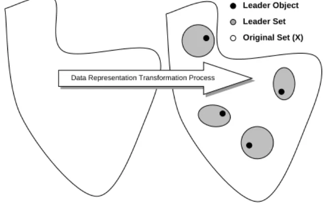
All family members (See Table-3.1), when applied to the original data set X, must:

• _{reduce X by selecting a set of representative objects}1_{, as typified in Fig-4.1. It could} also be thought of that the “leader” is reducing the variability in the data. That is, trying to get to the core of the data set, rather than all of the minor perturbations. • _{satisfy a mathematical property, as exemplified in (4.1).}

• _{contend with the problem of incompleteness (missing data).}

• _{contend with the problem of data type heterogeneity. For an example of using} het-erogeneous time series data, see [18].

{(∀j ∈ [1, |X|])(∃i ∈ [1, |L|])s(~li, ~xj) ≥ Ts} = L(X, Ts) ⊆ X (4.1)

Leader Object Leader Set Original Set (X)

Data Representation Transformation Process

Figure 4.1: Conceptualization of Clustering Process

4.2 Visual Domain Models

4.2.1 Use Case

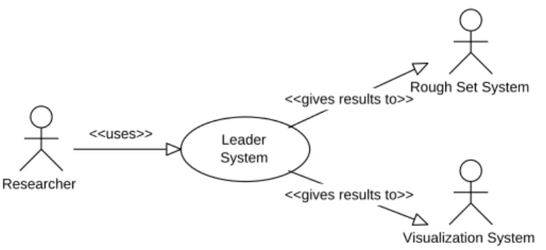
The way in which the Leader Algorithm System will be used is shown in Fig-4.2. In particular, one motivation of the system is to reduce the size of the data set when given to another system, and yet retain the core structure of the original data.

The focus of the project is testable feature contracts and their associated derived tests, so this use case was not elaborated further.

Definition 9 (Use Case) http://www.foruse.com/articles/structurestyle2.pdf states: Jacobsons original definition [Jacobson et al.,1992]: A use case is a specific way of using the system by using some part of the functionality. [A use case] constitutes a complete course of interaction that takes place between an actor and the system.

1_{cases and objects are used interchangeably}

(20)

Researcher

Leader System

Visualization System <<gives results to>>

<<gives results to>> <<uses>>

Rough Set System

Figure 4.2: Use Case (UC) for Leader Algorithm Family

The specification of sequences of actions, including variant sequences and error se-quences, that a system, subsystem, or class can perform by interacting with outside actors [Rumbaugh et al, 1999: 488].

[Fowler, 1997: 43]: A use case is a typical interaction between a user and a computer system [that] captures some user-visible function [and] achieves a discrete goal for the user.

Use cases ... are, of course, only one of many potential ways of modelling tasks, ranging from, on the one end of the spectrum, rigorous and highly structured approaches that are of greatest interest to researchers and academics, to, on the other end, informal movie-style storyboards and free-form scenarios.

From www.alike.com/html/main_html/glossary.html: A methodology used in system analysis to identify, clarify, and organize system requirements. The use case is made up of a set of possible sequences of interactions between systems and users in a particular environment and related to a particular goal. It consists of a group of elements (for example, classes and interfaces) that can be used together in a way that will have an effect larger than the sum of the separate elements combined. The use case should contain all system activities that have significance to the users.

4.2.2 Use Case Maps

The use case map in Fig-4.3 represents the responsibilities within the Leader Algorithm System that was implemented. The UCM also maps the responsibilities onto abstract con-ceptual components. For example, in Fig-4.3 the Object Presentation Order responsibility is mapped onto an abstract component called Preprocessing, which in turn may be mapped onto a concrete component or components in a particular family member2.

The mapping from abstract components to concrete components is described in §5, along with other details of the project implementation work.

Definition 10 (Use Case Map - UCM) http://www.usecasemaps.org states: Use case maps can help you describe and understand emergent behaviour of complex and dynamic systems.

2_{The mapping from abstract component to concrete component may or may not be done in different}

ways for different family members.

(21)

Preprocessing

Algorithm

Postprocessing Object Presentation Order

Leader Set Search Order

Leader Selection

Output Report

Figure 4.3: Use Case Map (UCM) for Leader Algorithm Family

4.3 Textual Domain Model

Domain models may be represented visually or textually. Visual domain representations, as in the previous section, take advantage of natural human visual understanding, and so may possibly be favoured over textual representations in certain circumstances. However, textual representations may be favoured due to their ability to describe structured languages — natural [e.g. Inuktitut, which is the major language of the Circumpolar region stretching from Alaska to Greenland and the main language for Nunavut3], artificial [Tengwar, which was invented by J.R.R. Tolkien], or computer [Prolog, for programming in logic].

Definition 11 (Testable Feature Contracts) Testable feature contracts are a textual feature model of a domain, from which tests (hopefully) can be directly derived. Feature contracts address feature coupling through explicit recording of feature interactions and be-havioral dependencies between features. Summarized from course

4.3.1 Features and Parameters

How were the features in Table-4.1 and parameters in Table-4.2 of this domain chosen? Based on a perceived notion of what was directly related to the leader algorithm family, implying that the features may not completely cover the domain being modelled. How could the features be proved to cover the domain? No known answer exists, unless, possibly, if the domain is formally defined via, for example, axioms. What would happen if we have a domain, but were missing a feature? It depends on what feature was missing. If enough other information existed in the model, then the missing feature could be derived from the other information, then possibly a tool could be built to help in this regard. However, in the general case, the missing feature will become apparent to someone with appropriate domain knowledge and then the correction will be made. Such latent changes incur potentially high cost. One advantage of feature contracts could be to try and find such missing features via the structured derivation of tests, forcing the model builder to more thoroughly consider the domain and ask the “right” questions of the “right” experts. What if we had a feature that wasn’t really a part of the domain? This should be found as long as the domain was

3_{Information obtained from the National Research Council Canada’s Interactive Information Group’s}

web site http://iit-iti.nrc-cnrc.gc.ca/projects-projets/uqausiit e.html

(22)

clearly understood and bounded, or the domain could be enlarged or shrunken to include or exclude that feature.

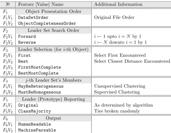
№ _{Feature [Value] Name} _{Additional Information} F1 Object Presentation Order

F1V1 DataSetOrder Original File Order

F1V2 ObjectCompletenessOrder

F2 Leader Set Search Order

F2V1 Forward i ← 1 upto i = N by 1

F2V2 Reverse i ← N downto i = 1 by 1

F3 Leader Selection (for i-th Object)

F3V1 First Select First Encountered

F3V2 Best Select Closest Distance Encountered

F3V3 FirstMostComplete

F3V4 BestMostComplete

F4 j-th Leader Set’s Members

F4V1 MayBeHeterogeneous Unsupervised Clustering

F4V2 MustBeHomogeneous Supervised Clustering

F5 Leader (Prototype) Reporting

F5V1 Original As determined by algorithm

F5V2 ClassMajority Ties broken randomly

F6 Output

F6V1 HumanReadable

F6V2 MachineParsable

Table 4.1: Feature and Feature Value Identifiers. F1V2 means feature value 2 of feature 1. Or put

another way, the 2nd _{possible variant of the feature.}

Definition 12 (Parameter) From the Ring Election thesis p47: a parameter defines a meaningful attribute input to the system. Contrary to a feature, we view a parameter not as a functional unit, but as a datum (e.g. length or weight). A feature may have parameters associated with it. These parameters may fully or only partially define a feature.

The possible binary interactions are listed in Table-4.3 and the mapping of features onto family members is list in Table-4.4.

(23)

№ _{Parameter [Value] Name} _{Additional Information} P1 ThresholdType See §5.1

P1V1 DistanceThreshold Td (used for DistanceFunction)

P1V2 DissimilarityThreshold (used for DissimilarityFunction)

P1V3 SimilarityThreshold Ts (used for SimilarityFunction)

P2 FunctionType See §5.1

P2V1 DistanceFunction

P2V2 DissimilarityFunction

P2V3 SimilarityFunction

P3 SortType

P3V1 StableSort Input order preserving sort

P3V2 UnstableSort Ties may be ordered in any way

P4 DataUsage

P4V1 OneCopyOfData Only one copy of the data exists

P4V2 MultipleCopiesOfData There may be multiple copies of the data

P5 MemoryUsage

P5V1 PrimaryMemory All data is loaded

P5V2 ExternalMemory Not all data loaded

P6 DistributionType

P6V1 UniformRandom f (x, A, B) = _B−A1

P6V2 Gaussian f (x, µ, σ) = e

−(x−µ)2/(2σ2)

σ√2π (Also called Normal)

P6V3 Poisson p(x, λ) = e −λ_λx x! for x = 0, 1, 2, · · · P7 SoftwareSystem P7V1 VisualizationSystem See [19] P7V2 RoughSetSystem See [19] P8 Computer P8V1 Sequential P8V2 Distributed See [2] P8V3 Parallel See [2]

Table 4.2: Parameter and Parameter Value Identifiers. P1V2means parameter value 2 of parameter

1. Or put another way, the 2nd_{possible variant of the parameter.}

(24)

№ _{Interaction Description}

X₀ applicable (e.g. not applicable ✗0)

X₁ is equivalent to X₂ requires X₃ has X₄ must be before X₅ is the parent of X₆ with

Table 4.3: Possible binary relations (interactions) that may occur. Not all are used in modelling this domain, the table certainly does not contain all possible relations, and no higher order (e.g. tertiary etc.) relations are proposed. The negation of the relation may be used ✗1. In general

ℜ_(F1, F2V2) means that F1is related to F2V2in the manner specified by the traceability code ℜ. In

particular, ✗3would mean does not have and X4,5would mean the conjunction of two interactions;

in this case, must be before –and– is the parent of.

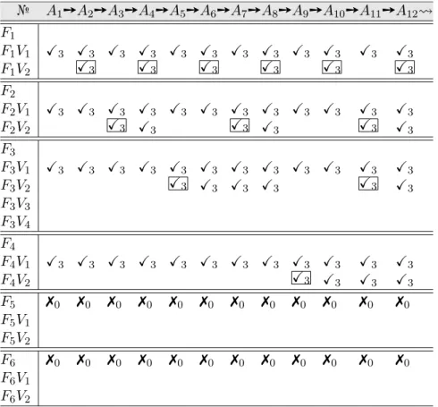
№ _A₁➙_A₂➙_A₃➙_A₄➙_A₅➙_A₆➙_A₇➙_A₈➙_A₉➙_A₁₀➙_A₁₁➙_A₁₂ F1 F1V1 X3 X3 X3 X3 X3 X3 X3 X3 X3 X3 X3 X3 F1V2 X3 X3 X3 X3 X3 X3 F2 F2V1 X3 X3 X3 X3 X3 X3 X3 X3 X3 X3 X3 X3 F2V2 X3 X3 X3 X3 X3 X3 F3 F3V1 X3 X3 X3 X3 X3 X3 X3 X3 X3 X3 X3 X3 F3V2 X3 X3 X3 X3 X3 X3 F3V3 F3V4 F4 F4V1 X3 X3 X3 X3 X3 X3 X3 X3 X3 X3 X3 X3 F4V2 X3 X3 X3 X3 F5 ✗0 ✗0 ✗0 ✗0 ✗0 ✗0 ✗0 ✗0 ✗0 ✗0 ✗0 ✗0 F5V1 F5V2 F6 ✗0 ✗0 ✗0 ✗0 ✗0 ✗0 ✗0 ✗0 ✗0 ✗0 ✗0 ✗0 F6V1 F6V2

Table 4.4: Member–Feature Relationships. For example, X3(A1,F1V1) means algorithm A1 has

the feature variant F1V1. The table has been designed based on ideas from John Tukey 1977. (For

example, the most important data and relationships should clearly stand out in a visualization.)

(25)

4.4 Changes to Feature Contracts

Changes (semantic/syntactic/presentation) were made to the feature contracts proposed in the course in order to simplify the applicability for the Leader Algorithm Family domain.

C1 Overall, tried to make section names like attributes of a feature that can be referenced. For example, a feature contract could be thought of like an interface.

C2 Removed superfluous textual strings (e.g. Interaction and Behaviour) because the meaning of a section (such as Variants) implies that it is an interaction or a behav-iour. This assumes that the reader understands what a section means.

C3 In Variation section, removed < type >∈. Old idea was F1.type and it has been

replaced by the ability to refer to a variant of a feature by using Variant_{. For}

example, the current variant of Feature 1, may be referred to as F1.Variant from

another feature such as F2 and as Variant from within F1. The additional notation

of This.Variant_{is not needed because the feature that the reader is currently reading}

is always assumed to be This. Consequently, the syntax is simplified, and Variant

is thought of like an attribute of a feature that is instantiated with a value. Further, consistency is introduced because we don’t have many different aliases for what boils down to referring to a variant. This requires less cognitive stress on the reader as fewer things need to be explicitly remembered.

C4 Removed Contract section, as it is superfluous because this information can be determined within the Mapping section (by a tool, if needed).

C5 Renamed Mapping section to Interactions section in order to make it more clear that other features interact with this feature in the mentioned ways. Constraints is another possible word, but was rejected due to the fact that data interactions may occur. For example, see F3.Interactions section.

C6 Each section is thought of as being an ordered operation (like the production rules in an expert system). For example, the accumulation += operation in F5.Interactions

C7 Added a Description section to describe the feature in natural language.

C8 Moved old Description section to be contained within the Composition section. C9 Added details to Responsibilities section.

C10 Feature and parameter names must be unique. Avoids parameter-feature confusion. C11 Composition can be conditional. See, for example, F1.

C12 Added ability to specify a set of responsibilities via set notation in conjunction with a template for a responsibility name. See, for example, F3.Documentation for

leader algX Y().

C13 Overall, tried to remove obfuscating syntax, and allow broader understanding of the intention of a contract without having a reader remember the meaning of particular symbols. For example, the syntax of Pascal versus C.

C14 Removed use of Null. Instead used None. This is to move more towards a domain, and away from a computer language, because it is trivial for a computer scientist to understand Null, but not necessarily for a domain expert. This, of course, assumes that domain experts may read these feature contracts.

C15 Changed Parameters notation to be consistent with the set notation used. C16 Renamed Variation to Variants.

C17 Added separating lines around the identifier and name of the feature so that the feature can be seen easily in a document.

C18 Lined names of items up, and separated them from content of items. This allows one to scan quickly for a particular item, such as Variants.

(26)

4.4.1 Feature Contracts

One of the course goals is to investigate how to document both feature interactions4 _and

behavioral dependencies5. For example, Feature–Feature, Feature–Parameter and other configuration rules (combination rules) are described within the feature contracts.

When writing a particular feature contract, the Interactions section was interpreted as being all of those things in other features that constrain, or are used by, this feature. In particular, the converse way of interpreting this section was not used. That is, the Interactions _{section does not document those things in this feature that are used by} other features. For example, when constructing Fi, it may be constrained to a particular

variant, sayVariant_k _{because F}_j _{has a variant within a set of possibilities.}

The following feature contracts are a model for the project implementation work on the Leader Algorithm Family. In addition, some generalization was performed in order to conceive of possible variants that were not implemented.

F1: Object Presentation Order

Description: _{The objects may be presented to the main body of the leader algorithm in}

many different ways. For example, they may be presented in the order that they are read from a file, or they may be sorted using any total or-dering relation (which may be comprised of a partial order in conjunction with, for example, the data set order) over the objects.

Variants: _{{DataSetOrder, ObjectCompletenessOrder}} Interactions: _None

Parameters: Parameters_{={SortType,DataUsage,MemoryUsage}} Variant ∈ {ObjectCompletenessOrder} ⇒

Parameters_{={StableSort,OneCopyOfData,PrimaryMemory}} Variant ∈ {DataSetOrder} ⇒

Parameters=None

Documentation: _{sortMatrixf()}_{create a new, reordered data matrix}

[Matrixf]original matrix of floating point numbers (See Fig-5.1) [MatrixfOut]sorted version of the input matrix (Share same data, just different pointers)

[IndexPointers]sorted pointers to data objects (See Fig-5.4)

[IndexMap] identity map or mapping from index of [IndexPointers] to index of original data objects

[Bins]bin i contains i missing values (See Fig-5.3)

Composition: Composition_{={[Matrixf],[IndexMap]}} Variant ∈ {DataSetOrder} ⇒/

Composition+={[MatrixfOut],[IndexPointers],[Bins]} Responsibilities: _{sortMatrixf()} _{

create [MatrixfOut], [IndexPointers], [Bins] }

4_{Feature interactions pertain to how the selection of a variant for a feature constrains the selection of a}

variant for another feature. [From course]

5_{Behavioral dependencies pertain to how a service offered by a feature depends on a service of another}

feature. [From course]

(27)

F2: Leader Set Search Order

Description: _{The currently grown set of leaders (there are k of them) may be searched}

in many different ways when object i’s membership to a leader needs to be determined.

Variants: _{{Forward,Reverse}}

Interactions: _F₃_.Variant ∈ {Best,BestMostComplete} ⇒ Variant={Forward}

F3.Variant ∈ {BestMostComplete} ⇒ Interactions={F₁.[Bins]}

Parameters: _None

Documentation: _[start]_{first leader index to consider}

[stop]last leader index to consider

comparisonFcn()tests if there are more leaders to consider iterationFcn()increment or decrement an iteration variable

Composition: Composition_{={[start], [stop]}} Responsibilities: _{comparisonFcn(){}

}

iterationFcn(){ }

(28)

F3: Leader Selection (for i-th Object)

Description: _{There are many ways to chose a leader to represent an object. The case}

of choosing multiple leaders for an object is not considered, therefore, exactly one leader will be chosen for object i. For all variants, if no leader in the current leader set exists that is close enough to object i, then object i will be promoted to becoming a leader, and hence selected as the leader for object i.

Variants: _{{First,Best,FirstMostComplete,BestMostComplete}6_} Interactions: Interactions _{= {F}₁_.[IndexMap]}

Variant ∈ {BestMostComplete} ⇒ Interactions += {F₁.[Bins]}

F4.Variant ∈ {MustBeHomogeneous} ⇒

Interactions += {F₁.[IndexMap].[ClassInfo]} Parameters: _{{DistanceThreshold,DistanceFunction}}

Documentation: _[k]_{cardinality of the leader set at any given point in time}

[P]object to leader mapping. (P [i] = j, case i is assigned to cluster j) has size exactly equal to the number of objects

[L]the leader set. (L[j] = i, cluster j is represented by object i) has size exactly equal to [k] with elements being objects from the input data set The [IndexPointers] are (polymorphically) represented as a [Matrixf]. This frees the implementation of this feature from having to know about the existence of F1, and therefore reduces feature coupling.

leader algX Y()where

{(X, Y )} = {(1, hartigan), (3, ext2), (5, ext4), · · · , (11, ext10)}

Composition: Composition_{={[k],[P],[L]}} Responsibilities: _{leader algX Y(){}

See Table-4.4 for details }

6_{This has not been implemented due to time constraints of the project. This variant considers all objects}

in bin j before bin j + 1. For example, if leader L1has 2 missing values and another leader L2has no missing

values, and if L1was “closer” than L2 to object i, then L2 should still be selected even though it is not the

first encountered because it has fewer missing values... making it the “better” choice.

(29)

F4: j-th Leader Set’s Members

Description: _{An object’s class may be used as additional information when considering}

adding it to the membership of a particular leader’s members. In partic-ular, the classes of all of the member objects belonging to a leader may be heterogeneous (i.e. the class information is ignored) or the object’s classes must be homogeneous.

Variants: _{{MayBeHeterogeneous,MustBeHomogeneous}} Interactions: _{F₁_{.[IndexMap].[ClassInfo]}}

Parameters: _None

Documentation: _{leader algX Y()}_{contains implementation} Composition: Composition_={}

Responsibilities: _{leader algX Y() where}

{(X, Y )} = {(1, hartigan), (2, ext1), (3, ext2), · · · , (12, ext11)}

F5: Leader (Prototype) Reporting

Description: _{The leader representative may be reported as being the same as what}

was originally selected, or if the data contains class information and the object members of a leader have heterogeneous classes, then the most abundant class may be chosen as a better representative of the set.

Variants: _{{Original, ClassMajority}} Interactions: Interactions_={F₁_.[IndexMap]}

F4.Variant ∈ {MustBeHomogeneous} ⇒

Interactions += {F₁.[IndexMap].[ClassInfo]} Parameters: _None

Documentation: _utility()_{contains implementation} Composition: Composition_={}

Responsibilities: _utility() _{

}

(30)

F6: Output

Description: _{The output from the Leader Algorithm System may be intended to be read}

by a human or parsed by another computer program with the purpose of further analyzing the original input data set.

Variants: _{{HumanReadable, MachineParsable}} Interactions: Interactions_={F₅_.utility()}

Parameters: _None

Documentation: _{createHumanReadableReportForASCII()}_{text-based report}

createHumanReadableReportForLaTeX()LA_{TEX-based report}

createMachineReadableReportForOptions()system options database createMachineReadableReportForData()leader database

Composition: Composition_={} Responsibilities: _{createHumanReadableReportForASCII()} _{ uses F5.utility() } createHumanReadableReportForLaTeX() { uses F5.utility() } createMachineReadableReportForOptions() { } createMachineReadableReportForData() { }

4.5 Derived Tests (from Feature Contracts)

Now that documenting feature interactions and behavioral dependencies has been attempted via feature contracts7, the following tests may be derived. In particular, static tests may be derived from feature interactions, while dynamic tests may be derived from the behavioral dependencies. The intention is to systematically derive as many kinds of tests as possible, in such a way that the resulting set of tests are fully traceable (i.e. Each test can be justified because of such and such a reason).

Definition 13 (Algorithm) Prof. Nussbaum (Carleton) taught in COMP3804 that: An algorithm is a well defined computational procedure that takes some value, or set of val-ues as input and produces some value, or set of valval-ues, as output. An algorithm is correct if for every input sequence the algorithm: i) halts, and ii) produces a correct output. An incorrect algorithm may: i) never halt, or ii) may halt and produce an incorrect answer. And another variant of the definition is from the field of Cognitive Science ([15] p.5): Information processes that transform symbolic input structures into symbolic outputs can be defined in terms of syntactic structures of the inputs and outputs. Such information processes analyze the syntactic structures of inputs and build syntactically structured out-puts. Such information processes are also called algorithms. (p.6) An algorithm is defined completely in terms of processes that operate on a representation. The processes do not op-erate on the domain being represented. They are not even defined in terms of the meaning

7_{This is one of the course goals.}

(31)

of the representation, which is carried separately by the semantic mapping from the rep-resentation to the domain. An algorithm is a -formal- procedure or system, because it is defined in terms of the form of the representation rather than its meaning. It is purely a matter of manipulating patterns in the representation.

Definition 14 (Test) ([3] p.1112) states that a test could be (1) An activity in which a system or a component is executed under specified conditions, the results are observed or recorded, and an evaluation is made of some aspect of the system or component. (2) To conduct an activity as in (1). (3) A set of one or more test cases. (4) A set of one or more test procedures. (5) A set of one or more test cases and procedures [IEEE 610].

Definition 15 (Test case) ([3] p.1113) states that a test case is a set of inputs, execution conditions, and expected results developed for a particular objective. A representation or implementation that defines a pretest state of the IUT (Implementation Under Test —in this paper called a family member—) and its environment, test inputs or conditions, and the expected result.

(32)

4.6 Derived Tests

Tests of feature contracts were derived from the point of view a compiler error report. Only tests need to be written; tests should say what to test rather than how. No testcases need to be written, but some are included in the appendix. Examples of each kind of test are provided when applied to the Leader Algorithm feature contracts. Syntax checks are not included. For example, not closing a { or forgetting an = or ∈.

1. Ambiguous (feature and parameter) reference for: Name. If F1’s Variants is:

> Variant={DataSetOrder}

and if F6’s Parameters is:

> Parameters={DataSetOrder}

Then the following should be reported:

>Ambiguous (feature and parameter) reference for: {DataSetOrder}. 2. Invalid feature variant referenced: Name.

If F2’s Interactions is:

> F3.Variant ∈ {Bests,BestMostComplete} ⇒

Then the following should be reported: >Invalid feature variant referenced: Bests. Similar kinds of errors could also be specified for: >Invalid responsibility referenced: Name.

>Invalid data referenced: Name. 3. Reference before definition for: Name.

If F2’s Interactions is:

> F3.Variant ∈ {Best,BestMostComplete} ⇒ Variant+={Forward}

Then the following should be reported: >Reference before definition for: Variant+=.

Because it should beVariant=.

4. Expression can never be true: Name. If F2’s Interactions is:

> F3.Variant ∈ {Best,BestMostComplete} ⇒ Variant={Forward}

and If F3’s Interactions is:

> F4.Variant ∈ {MayBeHeterogeneous} ⇒ Variant={First}

> F4.Variant ∈ {MustBeHomogeneous} ⇒ Variant={FirstMostComplete}

Then the following should be reported:

>Expression can never be true: F3.Variant ∈ {Best,BestMostComplete}.

5. No documentation exists for: Name.

A list of data and responsibilities can be made, and then the Documentation section can be checked to ensure that all items are documented.

Similar kinds of errors could also be specified for: Not used outside documentation section: Name.

Responsibility not used anywhere other than definition: Name. Data not used anywhere other than definition: Name.

Parameter not used anywhere other than definition: Name.

(33)

6. Invalid variant combination. Leader = {F1, F2, F3, F4, F5, F6}

> Leader1 = {ObjectCompletenessOrder,Reverse,Best, MayBeHeterogeneous,ClassMajority,HumanReadable}

This is only only combination that was found to be illegal, because Reverse should be Forward. However, this is not quite true, because it is not an error to search Reverse because when combined with Best, all of the leader set needs to be considered. This condition was only put into the feature contract so that a feature combination could be demonstrated that was not valid.

There is not enough time to discuss in depth about pre- and post- conditions for the tests; nor for domain specific tests (See §5.4). A small list will merely be mentioned:

1. cardinality of k must always equal size of the leader set [L].

2. class information read from the data file must be in range < 1..NumClasses>, where NumClassesis data domain specific, but none-the-less, assumed to be contiguous. 3. in terms of vectors, the size of an int must always be less than or equal to the size

of a vector element. This is because an int is written to the bytes of an element. A different implementation is possible. For example, a mapping index for an element could be made such that it would allow constant time access to a vector of elements of non-uniform size (See §6.1).

4. the test code assumes that the class information is the last column in the data matrix. inputs->classIndex = size_matrixf_cols(inputs->data);

But it could be possible to add this information to the data matrix itself, thereby increasing flexibility for the user.

5. the count function used in the implementation of sort matrixf() must return an intvalue ∈ [0..size matrixf cols([Matrixf])]

6. there may not be enough memory 7. a file may not be openable, or writable

The appendix has a test case suite that demonstrates some of the differences between family members in the Leader Algorithm Family.

(34)

Chapter 5 Implementation

T

he implementation strategy was iterative. In particular, Hartigan’s algorithm was im-plemented first, and then additional features were added. This time dependance is illustrated in the heading of Table-4.4. The process (iterative, tightly integrated, small wa-terfalls, semi-automated testing) is illustrated as follows: i) consider one feature that was not in Hartigan’s algorithm, ii) extend Hartigan’s algorithm to incorporate this feature, iii) test the extension, iv) make a second extension by adding a preprocessing sort wrapper, v) test these extensions, vi) integrate these extensions into a larger algorithm that incorporates all features up until this point, and vii) then move on to the next feature.

5.1 Threshold Function

The only threshold function that is currently acceptable is a DistanceFunction. However, this is easily extended to support a SimilarityFunction by the addition of a parameter that specifies the comparison relation to use with respect to the threshold. As the focus of the project is not on the implementation of different DistanceFunction’s, but on the imple-mentation of the algorithm, it is left to the DistanceFunction impleimple-mentation to transform itself into a SimilarityFunction. For example, one possible similarity function that could be used is a non-linear transformation of a modified Euclidean distance (s = 1/(1+d), where s is a similarity and d a distance), accepting missing values (See [19], but originally from [5]). In particular, given two vectors ←−x =< x1, · · · , xn>, ←−y =< y1, · · · , yn>∈ Rn, defined by a

set of variables (i.e. attributes) A = {A1, · · · , An}, let Ac ⊆ A be the subset of attributes s.t.

xi 6= X and yi6= X. The corresponding distance function is de = (1/card(Ac))P_A_c(xi− yi)2.

This is a normalized distance and therefore, independent of the number of attributes. Con-sequently, no imputation of missing values to the data set is performed. See Table-5.1 for possible distance functions.

(35)

Modelling Variability in the Leader Algorithm Family Name Distance Euclidean Ac(xi−yi)2 card(Ac) Clark Ac (xi−yi)2 (xi+yi)2 card(Ac) Canberra Ac |xi−yi| (xi+yi) card(Ac) Others... ...

Table 5.1: Three possible modified distances ([19]p.1947)

(36)

5.2 UCM Component Mapping: Abstract → Concrete

The use case map (UCM) in Fig-4.3 contains abstract components wrapping the responsi-bilities. These components are implemented as concrete entities in the code. The mapping from abstract component to concrete component for each of the abstract components are listed in Table-5.2 for the Preprocessing abstract component, Table-5.3 for the Algorithm abstract component, and Table-5.4 for the Postprocessing abstract component.

matrix io.h matrixf read matrixf (FILE *f)

matrix sort.h void sort matrixf (matrixf m, matrixf* outM, vectori* outIndices) leader utils.h void swapDataAndSortedData(leader alg in t* inputs)

Table 5.2: Mapping of abstract preprocessing component to concrete components

leader utils.h void initSearchParms(leader alg in t* inputs, leader alg out t* outputs) leader.h void leader alg1 hartigan(leader alg in t* inputs, leader alg out t* outputs) leader.h void leader alg2 ext1(leader alg in t* inputs, leader alg out t* outputs) leader.h void leader alg3 ext2(leader alg in t* inputs, leader alg out t* outputs) leader.h void leader alg4 ext3(leader alg in t* inputs, leader alg out t* outputs) leader.h void leader alg5 ext4(leader alg in t* inputs, leader alg out t* outputs) leader.h void leader alg6 ext5(leader alg in t* inputs, leader alg out t* outputs) leader.h void leader alg7 ext6(leader alg in t* inputs, leader alg out t* outputs) leader.h void leader alg8 ext7(leader alg in t* inputs, leader alg out t* outputs) leader.h void leader alg9 ext8(leader alg in t* inputs, leader alg out t* outputs) leader.h void leader alg10 ext9(leader alg in t* inputs, leader alg out t* outputs) leader.h void leader alg11 ext10(leader alg in t* inputs, leader alg out t* outputs) leader.h void leader alg12 ext11(leader alg in t* inputs, leader alg out t* outputs)

Table 5.3: Mapping of abstract algorithm component to concrete components

leader io.h void write leader reports(

leader alg in t* inputs, leader alg out t* outputs, leader report t* rep)

Table 5.4: Mapping of abstract postprocessing component to concrete components

(37)

5.3 Design decisions

DD12004-OCT-05 A discussion between the author and Dr. Vald´es revolved around how sorting could be done efficiently. One possibility, which involves determining the number of missing values per data object and either appending to a completeness list or inserting into another list of varying incompleteness, is diagrammed in Fig-5.2. A second feasible implementation, which was selected because it is faster, is range sort, which is diagrammed in Fig-5.3.

DD22004-NOV-19 When outputting the leader algorithm report, because we may have sorted the data, we need to keep track of the original case numbers. To do this, an extra attribute on a data object has been added, namely a case identification number (indexed from 1). For example, the i-th case in the input data file will result in the construction of a data object containing all of the data from that case in addition to a case identifier equal to the value i. The design tradeoff is that a little bit more memory (sizeof (int)×numCases) will be used, versus a lot more computation to try to reverse map the case identifier for a particular data object in the sorted matrix. For example, one possible implementation might be via pointer equality, as the data objects don’t move in memory. However, this would require looking through the whole array multiple times. This design decision has ramifications because the additional data object’s case identification attribute can’t be used by i) a similarity or dissimilarity function, and ii) a data object completeness determination function.

DD32004-NOV-24 Upon further reflection, the idea of putting an additional attribute into a case when the data is read into memory is not the best way; it is better to remove the coupling between the indices and the data. The visual representation (shown in Fig-5.4) helped clarify and crystalize this concept into a more efficient implementation that allows i) use of the sorted data in algorithms that only know about the original data (See, for example, leader_alg4_ext3()) and ii) use of the indices by the reporting methods (See leader_io.c). Therefore, this deeper understanding has changed the previous design decision because the justification for the additional complexity for the similarity functions or data object completeness functions is not warranted.

Contiguous Memory Pointers to vectorf matrixf 0 1 2 3 ...

3 numRows numCols missingVal

numCols val val val val val ...

Figure 5.1: Abstract representation of a data matrix in primary memory.

(38)

Modelling Variability in the Leader Algorithm Family 1 2 3 ... k 1 2 3 . . . N

Object Processing Order

append insert 1 2 3 . . . N C I₊ -X

Figure 5.2: One variant of sorting incomplete data objects (X = CSI)

1 2 3 4 ... k Data in Memory 1 object 6 object 8 object i Count Function 2 3 object 1 object 3 4 object 2 5 6 object 5 7 8 object 7 ... object 4 object 9 k Count object i 0

Figure 5.3: Time efficient, O(2n), and space efficient, O(sizeof (int∗) × (n + k)), range sort of incomplete data objects using pointers.

... 2 3 4 5 6 7 ... Original Order 1 2 3 4 ... k Data in Memory ? 2 3 ? ... k Data in Memory ... 2 3 4 5 6 7 ... Incompleteness Order ... 7 3 4 2 6 5 ... Indices Pointers Pointers

Figure 5.4: Data in primary memory indexed in two different ways: i) by secondary storage (data file) order, and ii) by incompleteness relation (count of missing values) order. Pointers are needed so that a matrixf can be constructed and given to a leader algorithm for either type of data. For example, if the original data is sorted before the algorithm is executed then a mapping between the original order and the sorted order is needed. The indices are how such a mapping is recorded.

(39)

5.4 Dynamic “Code-based” Unit Tests

These tests were written -during- the iterative construction of the code, and so were not explicitly planned, but were an integrated, dynamic part of a robust (and creative) devel-opment process employed in a style similar to the x-treme manifesto, whereby small unit tests are written before the code. This is in contradistinction to tests derived from features, hence the separation from those more formally (feature model based) derived tests. In other words, these tests are directly based on the code, and are related very specifically to code development activity rather than to the much higher level of the domain modelling based testing activity.

UT12004-NOV-07 Implementing the sort function was intellectually stimulating.

UT22004-NOV-12 It was interesting that during the construction of the translation of Hartigan’s algorithm (See §3.1.1), line 4, which correctly reads, i ⇐ 2, was incorrectly translated to read i ⇐ 1, but this error was found during iterative testing while building the implementation, and so now the translation –may– be correct.

UT32004-NOV-19 When running an algorithm that did nothing, the expectation was that no leaders should have been formed, but which was not the case, as some leaders were being reported with some of them having values of 0, but others having values of 19,216 (a completely random value), both of which should not have occurred. Both of these errors (non-zero value and more than zero leaders) were curious, and so it was proposed that calloc (when dynamically allocating a vector allocate_vector) was not initializing the memory to zeros. This was proved false when the P vector was investigated, as it had all zeros. Therefore, it was proposed that possibly the algorithm was implemented incorrectly for updating k, but this was proved false by the fact that the algorithm worked correctly on a previous test. Then the interaction between successive calls to the algorithm (passed as a function pointer argument to runOneLeader) revealed that info was not being initialized correctly. In particular, void construct_leader_t(leader_t* info)did not initialize k to zero, but this was not originally performed, because it was assumed that k would be initialized inside the algorithm e.b. info->k = 1; inside leader_alg1_hartigan. So, in hindsight, this test was probably flawed, in that an algorithm that does nothing should never actually be executed, but on-the-other-hand the code is now a little bit more robust.

UT42004-NOV-24 It is important to use prefix notation when decrementing or increment-ing a integer variable in a return statement (e.g. return --i;).

UT52004-NOV-25 It was discovered that the number of columns was not being written to the data file correctly after implementation of DD3.

In particular, in the matrix_io_runTestSuite() the matrix_io_test_01() exhibited this failure. In order to fix this problem, it was noted that the code for implementing DD2 still existed, and so it was decided that all code related to that decision should be deleted because that code may have been buggy. After the code was deleted, matrix_io_test_01()then had the expected output. The bug was probably a minus 1 that should not have existed, but there was no reason to spend time to try to track it down due to the change in design decision, and hence, lack of corresponding justification.

UT62004-NOV-26 The output report does not contain the correct indices, which was discovered when running leader_testSuite.c while trying to complete the imple-mentation of DD3.

(40)

For example, L[2] |1| >3< [ 2] is clearly incorrect, because the selected >3< does not appear in the leader set, which only consists of the index 2. It was found that in createHumanReadableReportForASCII() the line which was previously written as algOutputtedIndex = ((vectori)rep->leaderSets[ii])[jj]; should actually be referenced through the index map i.e. inputs->data_sorted_map[...]. The offend-ing line now correctly reads L[2] |1| >3< [ 3].

UT72004-NOV-26 An access violation was occurring within leader_testSuite.c. It turns out that destroy_leader_alg_in_t() was implemented incorrectly. There were two problems: i) deallocate_matrixf_andData(inputs->data); was called before deallocate_matrixf_andData(inputs->data_sorted);, which should have been the other way around, and ii) when deallocating the sorted data, the call should not have been to the _andDat() variant, but to the _butNotData() variant.

These problems were found because the leader test suite tries more than one leader algorithm, and the particular algorithm that exhibited this problem was the extension that added the sorting capabilities. That is, the interaction between the sorting feature, and the leader algorithm were problematic.

UT82004-NOV-26 The output from leader_alg5_ext4() for the oneLeader case was incorrect. That is, P[1]=1 but P[2]=2, P[3]=2 and P[4]=2 and only one leader was expected. It was found that the implementation was incorrect. In particular, the line outputs->P[i] = j;should have been outputs->P[i] = bestDistanceIndex;

UT92004-NOV-28 inputs->distanceFcn(i,j,inputs) should have been implemented as inputs->distanceFcn(i,outputs->L[j],inputs). This was discovered while writ-ing the code for leader_alg9_ext8() and not from a particular test (although a test can be written for this case). In particular, the conceptual mistake was discovered when get_class_for_object_from_matrixf() was written for the homogeneous case, mainly due to the fact that the only distance function that has been implemented up until this point, is the constant distance function (i.e. a distance function that always returns the same value). This decision was made in order to focus the testing on those things that have been explicitly implemented because it is not necessary to test some-thing that hasn’t been implemented, as that test will always fail. However, it is now the correct moment in time for these tests to be implemented.

UT102004-DEC-15 When modifying the output in leader_io.c to be more informative, it was found that the vector outputs->L had an incorrect size, but that k was correct. This meant that memory was potentially being accessed when it should not. This was corrected in leader alg1 hartigan() and the other relevant leader algorithms.

Modelling Variability in the Leader Algorithm Family: A Testable Model and Implementation

NRC Publications Archive

Archives des publications du CNRC

Modelling Variability in the Leader Algorithm Family: A Testable Model

and Implementation

Barton, Alan

Modelling Variability in the Leader Algorithm

Family: A Testable Model and Implementation *

Barton, A.

December 2004

Modelling Variability in the Leader Algorithm Family:

A Testable Model and Implementation

Contents

List of Figures

List of Tables

List of Algorithms

Nomenclature

Chapter 1

Introduction

T

Chapter 2

Project

T

2.1

Project Conceptualization

2.2

Project Domain Scope

2.3

Project Constraints and Coverage

Chapter 3

Domain

C

3.1

Family Members

Chapter 4

System Family Engineering

Domain Models

T

4.1

Textual Domain Representation

4.2

Visual Domain Models

4.3

Textual Domain Model

4.4

Changes to Feature Contracts

4.5

Derived Tests (from Feature Contracts)

4.6

Derived Tests

Chapter 5

Implementation

T

5.1

Threshold Function

5.2

UCM Component Mapping: Abstract → Concrete

5.3

Design decisions

5.4

Dynamic “Code-based” Unit Tests