HAL Id: hal-01615232
https://hal-mines-paristech.archives-ouvertes.fr/hal-01615232
Submitted on 12 Oct 2017
HAL is a multi-disciplinary open access
archive for the deposit and dissemination of
sci-entific research documents, whether they are
pub-lished or not. The documents may come from
teaching and research institutions in France or
abroad, or from public or private research centers.
L’archive ouverte pluridisciplinaire HAL, est
destinée au dépôt et à la diffusion de documents
scientifiques de niveau recherche, publiés ou non,
émanant des établissements d’enseignement et de
recherche français ou étrangers, des laboratoires
publics ou privés.
Short-term Forecast of Automatic Frequency
Restoration Reserve from a Renewable Energy Based
Virtual Power Plant
Simon Camal, Andrea Michiorri, Georges Kariniotakis, Andreas Liebelt
To cite this version:
Simon Camal, Andrea Michiorri, Georges Kariniotakis, Andreas Liebelt. Short-term Forecast of
Auto-matic Frequency Restoration Reserve from a Renewable Energy Based Virtual Power Plant. The 7th
IEEE International Conference on Innovative Smart Grid Technologies - ISGT Europe 2017, IEEE
Power & Energy Society (PES), Sep 2017, Torino, Italy. pp.1-6, �10.1109/ISGTEurope.2017.8260311�.
�hal-01615232�
Short-term Forecast of Automatic Frequency
Restoration Reserve from a Renewable Energy Based
Virtual Power Plant
Simon Camal, Andrea Michiorri
Georges Kariniotakis
MINES ParisTech, PSL – Research University Center PERSEE
Sophia-Antipolis, France simon.camal@mines-paristech.fr
Andreas Liebelt
FRAUNHOFER Institute for Wind Energy and Energy System Technology IWES
Kassel, Germany
Abstract— This paper presents the initial findings on a new
forecast approach for ancillary services delivered by aggregated renewable power plants. The increasing penetration of distributed variable generators challenges grid reliability. Wind and photovoltaic power plants are technically able to provide ancillary services, but their stochastic behavior currently impedes their integration into reserve mechanisms. A methodology is developed to forecast the flexibility that a wind-photovoltaic aggregate can provide. A bivariate Kernel Density Estimator forecasts the probability to provide reserve. The methodology is tested on a case study where volumes of automatic Frequency Restoration Reserve (aFRR) are forecasted on a day-ahead horizon. It is found that the wind-photovoltaic aggregate can dedicate a limited share of its forecast production to aFRR. The frequency of insufficient reserve capacity is assessed, by comparing the capacities offered with the measured production.
Index Terms-- Aggregation, Ancillary Services, Forecasting,
Photovoltaics, Wind power.
I. INTRODUCTION
Variable renewable power plants substitute conventional synchronous generators at a fast growing rate. The increased intermittency among available generation impacts significantly the stability of power systems. Due to the spatiotemporal uncertainties associated with their production, variable renewable generators are currently restrained by operators in their provision of Ancillary Services (AS), for which maximum reliability is a firm pre-requisite. However studies have identified that wind and photovoltaics (PV) power plants show technical capabilities to provide AS [1],[2]. The Irish TSO has issued a specific regulation for frequency control from wind power plants [3]. This paper investigates the capacity of renewables to offer frequency control services.
Frequency control services follow a multi-level sequence. At a first control level (activation time 0-5 s), the inertia of generators contains instantaneous frequency perturbations.
Wind and solar plants can emulate synthetic inertia [1]. The next level is Frequency Control Reserve (FCR), where generators connected to a synchronous area regulate their power output in function of the frequency deviations they capture. Frequency Restoration Reserve (FRR) follows FCR. It is activated both automatically (aFRR, full activation time 5-15 min) and manually (mFRR, full activation time 13-15 min). TSOs activate aFRR by first evaluating centrally the Area Control Error, then calling for modification of the active-power setpoint of generators. In France, the TSO updates the aFRR sizing at a 30-min timestep [4]. The amount of aFRR is expected to vary in the coming years: the International Grid Control Cooperation, triggered by European TSOs, increases its exchanges in order to lower the overall need for aFRR [5]. In contrast, the stochastic behavior of renewables is expected to lead to higher aFRR levels. Improvement in wind and solar power forecasting could mitigate their impact on the sizing of this reserve [6]. The last level of response to frequency deviations is Replacement Reserve (RR) which is in place in several European countries. RR is manually activated in case the restoration reserve is not sufficient to ensure stability, within a time frame of 15 to 30 min.
Procurement schemes and markets for AS are diverse among European countries. Some services may be mandatory in some countries (e.g. FCR, [7]), tendered following economic merit-order (RR in France, [4]), or traded on a market with different upward and downward prices (RR in Portugal, [8]). For an energy trader, participation in reserve markets is economically interesting if the reserve price is superior to the average price for energy. While current prices in Europe tend to incentivize more energy than reserve [6], the AS markets are profoundly evolving and promising for renewables as their marginal cost is close to zero. Bidding strategies for participation of wind farms in an AS market have been studied recently. The reserve strategies proposed in [9] keep a share of the active power forecast to the FCR market. The optimal bid of wind power is analytically derived as a quantile of the production forecast for the day ahead,
This work is realized within the frame of the European project REstable, supported by the ERA-NET Smart Grid Plus program with the financial contribution of the European Commission, ADEME and Jülich Research Center.
considering high penalties in the balancing market if failing to provide the FCR service. Moderate increase in revenue is found (<12%) compared to participation in energy market only.
The European project REstable, which motivates this paper, aims at demonstrating renewable-based ancillary services through better interaction of European control zones [10]. The central idea of the project is that the aggregation of distributed power plants with distinct features (geography, time, resource, market regulations) can offer reliable AS via an adaptive European Virtual Power Plant (VPP).
Reliable offers of AS suppose adequate power forecasting methods. For variable generation, assuming that the distribution of forecast errors depends only on historic performance does not capture the uncertainty inherent to the forecast model [11]. The nonlinearity of wind and solar generation induces that conditional distribution of forecast errors is easier to model with nonparametric approaches [12]. According to a review of probabilistic methods for reserve requirements [11], density forecasts can be applied to both wind and solar power, and give more reliability on reserve allocation problems than approaches based on historical forecast only. Kernel Density Estimation (KDE) is a density forecast method which figures among the top-ranked methods for wind and PV forecasting [13]. Ensemble forecasts represent an alternative to density forecasts. They can incorporate temporal and spatial interdependence of prediction errors, and perform well on short-term horizons [14]. A density approach has been chosen here to model the problem of aFRR capacity forecasting, formulated in Section II. The forecast method is described in Section III.
II. PROBLEM FORMULATION
The objective of this work is to forecast a reliable day-ahead offer of aFRR, provided by a VPP aggregating photovoltaic and wind power plants located in France. This geographical limitation is due to the availability of data for tests. It is deemed acceptable to study a VPP concerned by the French control area, because most of the aFRR need in France is covered currently by plants located within this area [15]. Producers who supply aFRR must comply with strict regulations defined by TSOs. For instance, German TSOs ask that deployed reserve capacities are never lower than the contracted volume over the whole product length [16]. In France penalties apply if the measured deployed capacity is more than 10% lower than the contracted capacity, over an evaluation period > 100 h [4].
This problem poses two main challenges:
1. Propose a reliable production forecast over the product length, so that the risk of failing to provide reserve due to overestimation of production is minimal.
2. From this forecast, derive volumes of reserve that are significant (superior or equal to 1% of aggregated capacity) during intervals of sufficient production.
The temporal resolution of the forecast must be at least equal to the temporal resolution of the AS product, in order to
qualify the aggregate as a potential AS provider. In the case of aFRR it is 15 minutes in Germany and 30 minutes in France. The production forecast has generally a coarser temporal resolution than the grid signals that the service must react to (e.g. Automatic Generation Control (AGC) signal). It also does not capture the very-short term variations in the power output of the aggregate. The forecasting error is therefore dependent on the temporal resolution.
It is assumed in the present study that plants can effectively communicate to a distant VPP control center and regulate their power output following setpoints sent by the center without significant discrepancies. Experiments conducted within the project Kombikraftwerk 2 have shown that renewable plants can be controlled within a 3-second time lapse. Power regulation of aggregated plants showed also some limits: regulation was unsuccessful on wind turbines operating close to cut-in wind speed, and deviated from the emulated AGC signal [17], similarly to another experiment [16]. In the next section, a methodology is presented to solve the afore-mentioned problem. Three approaches are proposed with increasing level of complexity: a basic approach using individual probabilistic production forecasts as inputs, a deterministic aggregated forecast issued by a bivariate KDE, and a probabilistic forecast computed by the same KDE model.
III. METHODOLOGY
A. Basic Approach for Aggregated Flexibility Forecast 1) Probabilistic production forecasts at plant level
Probabilistic production forecasts are issued for each plant of the aggregate. The forecasts are based on a KDE k-Nearest Neighbors (k-NN) model for PV plants, and bivariate conditional KDE on wind speed and wind direction for Wind plants. A description of the k-NN algorithm is reported in Subsection B.3. Both forecasting models have been validated using deterministic and probabilistic criteria [18], [19]. The forecasts are issued at a runtime t for a horizon interval ∆h.
2) Individual flexibility forecasts at plant level
For each plant of the aggregate, a share of the active power forecast is dedicated to reserve. This target share is considered here as a quantile of the probabilistic forecast, at nominal value α. The choice of the nominal value α can be realized through an optimization on expected gains and losses associated with energy and reserve, similarly to optimal bidding strategies used by renewable producers [20].The risk of failing to provide reserve decreases with α. The total reserve volume is then chosen as the minimum value of the quantile on the horizon interval ∆h of the day to predict. The minimum is chosen in (1) to minimize the risk of failure. The offer of symmetrical reserve rˆ by the plant i at runtime t, is i,t
equal to half of the total reserve volume:
( )
α = − + ∆ ∈ ∀ 1 , , min 2 1 ˆ it ht h h t i F r(1)
where
F
i,−t1+ th is the inverse Cumulative Distribution Function (CDF) of the power forecast of plant i at horizon h.3) Aggregation of Individual Flexibility Forecasts
The aggregated day-ahead offer rˆt issued at runtime t equals in (2) to the sum of the individual forecasts from the plants of the aggregate.
∑
= = plants N i t i t r r 1 , ˆ ˆ (2)B. Aggregated KDE Probabilistic Forecast
In this section, a bivariate KDE model is proposed to forecast the power production of an aggregate of PV plants and Wind plants. Weather conditions are reduced to a joint distribution of solar radiation and wind speed, therefore this model applies to aggregates in which plants of same technology experience similar weather conditions. Future work could include more diversity in weather forecasts via reduction techniques such as Principal Component Analysis (PCA), or ensembles using weather forecast at multiple sites.
1) Retrieve weather forecasts and select reference data
In this work, a central reference site is derived for all plants of similar technology. The coordinates of the site minimize Euclidean distance among plants. Numerical Weather Prediction forecasts (NWP) are retrieved for the reference sites. For photovoltaic plants, a unique NWP, Solar Surface Radiation Downwards, is selected. For Wind plants, meridional and zonal wind components are selected as they appear in the literature to be the principal influential variables [19], [21], [22].
2) Select bi-variate conditional explanatory variables
The bivariate explanatory variable , based on NWP forecasts, is constructed in (3) following a simple regime-switching approach. The contribution of solar radiation to the bi-variate condition at the current timestamp is estimated by
0 ,
I
w , the proportion of PV power installed in the aggregate. This static contribution is associated to the contribution wˆI
of the solar radiation forecast Iˆ , which is compared to its expected value over the available learning data set E(Iˆ):
) ˆ ( ˆ ˆ , , ˆ . , , 0 , 0 , I E I w P P w w w w I peak aggreg peak PV I I I I = = = ) ˆ , ˆ ( ), ˆ , ˆ ( ,0 0 , X I W w w X U V w wI > I ⇒ = I ≤ I ⇒ = (3)
where Wˆ is the wind speed, Uˆ and Vˆ the meridional and zonal wind components respectively.
3) Training data selection by k-Nearest Neighbours
The estimator is trained on a sample of similar bivariate points of NWP forecast, following a NN approach. The k-NN algorithm has been applied to probabilistic wind power forecasting [21], [22], and has the advantage of maintaining constant the size of the training data as new forecasts are added [12]. Nearest neighbors minimize in (4) the Manhattan Distance between the available historical learning set X and the forecast condition x. Distances are weighted by the contributions of PV and Wind in the case where solar contribution is significant. The weights for meridional and
zonal wind components wU and wV , are obtained via an optimization on the sum of square errors from the deterministic output of the KDE, presented in the next section. The optimization is realized with a Particle Swarm Optimization algorithm [23], following a cross-validation on weekdays as presented by [21]. ≤ − + − > − + − = 0 , 0 , , ) .( ) .( , ) .( ) .( ) , ( I I V V V U U U I I W W W I I I w w X x w X x w w w X x w X x w X x D (4)
The training set is populated in (5) with nearest neighbors until the set size kT has reached a ratio rkNNof the size of the learning set L. An upper bound of 125 is applied to contain computational burden. Such a value appears sufficient in the context of k-NN wind power forecasting [21].
(
)
{
, ,}
, 125 . ∈ ≤ = kNN k k T T r Card X Y k L k k (5)4) Conditional Kernel Density Estimator
The obtained training sample of conditional explanatory variable is compared to the forecast condition x within a bi-variate KDE, with the Kernel proposed in [19]. A bandwidth matrix H is computed following the Smooth Cross Validation (SCV) method to model directions of correlation between covariates [24]. In conditions when wind is dominant, a diagonal SCV matrix is selected. The explanatory weight wˆX
in (6) associates the weather forecast condition x with its position relative to the learning set of size N, and filters older points by an exponential forgetting factor fgt of constant parameter λ.
(
)
( )
(
(
)
)
(
)
(
)
∑
= − − − − λ = N j j X X x H K X x H K fgt X x w 1 1 1 . , ˆ (6)The conditional density forecast of aggregated production
t h
t X
Y
fˆ + is obtained in (7) via a KDE with a bandwidth hY
equal to the k-nearest neighbour, using the same ratio rkNN. An Epanechnikov Kernel and a reflection method model the bounded behavior of the production.
( )
(
)
− =∑
= + Y i Y N i i X Y X Y h y y K X x w h x y f t h t 1 , ˆ . 1 , ˆ (7)5) Selection of minimal quantile of aggregated forecast
The forecast flexibility offer rˆt is chosen in (8) as the minimum of the aggregate production for the α-quantile, on the horizon interval ∆h of the day to predict.
( )
α = −+ ∆ ∈ ∀ 1 min 2 1 ˆ t ht h h t F r (8)C. Aggregated Deterministic Forecast
The third approach uses the KDE model presented in Section B to derive an aggregated deterministic forecast. Predictive densities produced by the model are optimized with respect to the expectancy E, so the mean of the predictive density for each horizon constitutes the
deterministic forecast. The forecast flexibility for the day-ahead horizon is chosen in (9) as the minimum of the deterministic aggregated forecast on the day to predict.
(
Yt hXt)
h h t E f r + ∆ ∈ ∀ = min ˆ 2 1 ˆ (9)IV. CASE STUDY
A. Workflow
The methodology is evaluated on the following case study. A VPP is constituted by 2 wind farms located in North-East France and 10 photovoltaic plants located in a region of West France. The wind farms account for 95% of the aggregated power capacity. The VPP offers symmetrical aFRR on a day-ahead horizon. Offers must be communicated to the TSO prior to 13:00 UTC, similarly to the existing rules in France [4]. Offered volumes of reserve are computed given the three approaches described in the methodology, for each day of the test period (December-January). The nominal value α of the production quantile forecast is set to 10%, for the individual plants and the aggregate. Note that only the amount of power proposed in the offer is calculated in this paper, not the price.
B. Input Data
Measured production from all plants is available at a 5-min resolution. Forecasts of solar radiation, meridional and zonal wind speeds at 100-m hub height are retrieved at runtime 12:00 UTC from ECMWF HRES, for horizons +12 h to +36 h.
C. Performance Indicators
The KDE aggregated forecast is evaluated using the following criteria: Root Mean Square Error (RMSE) for its deterministic version, reliability and Continuous Ranking Probability Score (CRPS) for the probabilistic version. Reliability informs on the probabilistic bias of the forecast while the CRPS produces an overall probabilistic forecast score [20]. We normalize here errors by the sum of the installed capacities in the VPP.
The risk of failing to provide offered reserve levels is evaluated with a simple criterion. If the measured production is lower than the offered reserve levels at a given timestamp, then this event is counted as an under-fulfillment. The Rate of
Under-Fulfillments (RUF) is the frequency of under-fulfillments on the evaluation interval. The RUF is chosen as
a criterion to assess the reliability of the ancillary service forecast. It is inspired by current practice of TSOs, eg. in France where aFRR deployment is judged insufficient if the reserve deployed is below the day-ahead offered capacity – 10%, during more than 10% of the evaluation interval [4]. The accuracy of this criterion is limited by the temporal resolution of the measured production. The amount of flexibility offered is another performance indicator. It is expressed by the Cumulated Distribution Function (CDF) of the volumes on the evaluation interval.
V. RESULTS
A. KDE Aggregated Production Forecast
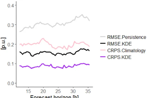
The training period of the KDE forecast is July– November and the test period is December – February. The forecast model issues predictions at a 30-min resolution over a 12-h to 36-h horizon. The deterministic output of the KDE aggregated forecast shows a RMSE comprised between 10% and 20% over the forecast horizon, with significant improvement compared to persistence (Fig. 1). These levels are coherent with state-of-the art forecasting for wind and PV at these horizons [18], [21]. The CRPS is comprised between 7% and 11% over the forecast horizon, with similar improvement compared to climatology.
The reliability of the probabilistic KDE forecast is evaluated by a calibration diagram (Fig. 2). The model shows fair reliability, in particular for the 10%-quantile, which is of particular interest for the present application. The calibration analysis shows room for improvement of the model, and could be extended to larger intervals.
Fig. 1: RMSE of deterministic KDE forecast and Persistence model. CRPS of probabilistic KDE forecast and Climatology model.
Fig. 2: Calibration diagram (over all horizons)
B. aFRR Offer Forecast
The offers of aFRR flexibility obtained with the three approaches are presented on an interval of high wind production in Fig. 3. The basic approach based on individual flexibility forecasts, in red on Fig. 3, offers volumes mostly inferior to 1% p.u., except when the forecasted production is constantly high during the whole day. The approach based on aggregated deterministic forecasts, in brown, leads to higher
flexibility levels, greater than zero for most of the days tested. Finally, the approach based on the aggregated probabilistic forecast, in orange, differs slightly from the individual forecast approach because it models the correlation between plants: its average flexibility is higher, whereas the dispersion of levels around the average is lower than for the individual forecast approach. Note that in the present day-ahead framework, the individual flexibility offered by PV plants is zero (no production at night).
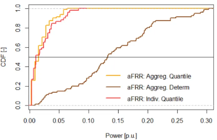
The CDFs of aFRR offers for the three approaches show that the potential offer levels span from 0 to 0.30 p.u. on the evaluation interval (Fig. 4). The median offers of the probabilistic approaches are 0.015 p.u. and 0.010 p.u., for the aggregated approach and the individual approach respectively. The cumulated Rate of Under-Fulfillment (RUF) compared to 5-min monitored production reaches 26% for the deterministic approach (Fig. 5). The cumulated RUF for the aggregated forecast approach is 7%, close to the 5% for the individual forecast approach. As a first conclusion, the probabilistic approaches appear to be better candidates than the deterministic approach for a reliable aFRR capacity forecast.
VI. DISCUSSION AND CONCLUSION
A bivariate KDE has been developed to predict an aggregated production of wind and PV plants, with encouraging results and insights for future improvements, especially on calibration. Optimization of the model for conditions with significant solar radiation could improve reliability. Other models such as Quantile Regression Forests, gradient boosting and copulas will be tested to forecast the aggregated production. Improvement of the aggregated production forecast, as well as shorter product length, would
lower the risk of failing to provide reserve. The aggregated flexibility forecast approach helps formulate offers for product lengths superior or equal to 24h: the individual forecast approach will lead to zero levels for PV plants (zero production at night). With high-resolution measurements of production data and weather conditions on site, the response of a VPP to frequency deviations or AGC signals can be modeled, and the probability of failure to deploy reserve can be assessed.
The rates of under-fulfillment observed in the case study could be assessed on a larger framework: higher plant diversity in the aggregate (higher PV penetration, several climates per technology), combined offers of aFRR with FCR. This would help calibrate the qualification tests a renewable aggregate must pass to provide AS. Future work may include conditional analysis on the technical capacity of an aggregate to deliver AS. Finally the Rate of Under-Fulfillment can be optimized given prices for energy and reserve.
A methodology to forecast the provision of aFRR by aggregates of wind and photovoltaic plants has been presented. Reserve levels are obtained through a simple minimal quantile selection on the production forecast. It is found that renewable power plants can offer volumes of automatic Frequency Restoration Reserve on a day-ahead mechanism, if their aggregate production is forecasted accurately. A trade-off is noticed between the volume of flexibility offered and the expected RUF. Potential aFRR capacities are identified on a case study, yielding volumes from 0 to 0.30 p.u. with medians of 0.01 to 0.13 p.u (Fig. 4).
Fig. 4: CDFs of aFRR offers for the three approaches
Fig. 5: Rate of Under-Fulfilment of aFRR for the three approaches
ACKNOWLEDGMENT
The authors wish to thank the contribution of HESPUL and ENGIE GREEN for the provision of historical production data and ECMWF for the provision of meteorological forecasts.
REFERENCES
[1] M. Faiella, T. Hennig, N. A. Cutululis, and F. Van Hulle, “Capabilities and costs for ancillary services provision by wind power plants,” ReServices Project Deliverable, 2013. [Online]. Available: http://orbit.dtu.dk/fedora/objects/orbit:127131/datastreams/file_ac1a56 c2-b722-439b-bcfb-fb6790c1f4fc/content
[2] B. I. Craciun, T. Kerekes, D. Sera, and R. Teodorescu, “Frequency Support Functions in Large PV Power Plants With Active Power Reserves,” IEEE J. Emerg. Sel. Top. Power Electron., vol. 2, no. 4, pp. 849–858, décembre 2014.
[3] Eirgrid, Eirgrid Grid Code. 2015.
[4] RTE, Règles Services Système Fréquence. 2017. [Online]. Available:
https://clients.rte-france.com/htm/fr/offre/telecharge/20170101_Regles_services_system e_frequence.pdf
[5] IGCC Expert Group, “Stakeholder document for the principles of
IGCC,” Sep. 2016. [Online]. Available:
https://www.entsoe.eu/Documents/Network%20codes%20documents/I mplementation/IGCC/20161020_IGCC_Stakeholder_document.pdf
[6] L. Hirth and I. Ziegenhagen, “Balancing power and variable renewables: Three links,” Renew. Sustain. Energy Rev., vol. 50, pp. 1035–1051, Oct. 2015.
[7] ENTSO-E, “Survey on Ancillary services procurement, Balancing market design 2015,” May 2016. [Online]. Available: https://www.entsoe.eu/Documents/Publications/Market%20Committee %20publications/WGAS%20Survey_04.05.2016_final_publication_v2 .pdf?Web=1
[8] ERSE, Manual de Procedimentos da Gestão Global do Sistema do Setor Elétrico. 2014. [Online]. Available: http://www.mercado.ren.pt/PT/Electr/InfoMercado/DocReg/BibSubreg ula/MP_GGS_SE.pdf
[9] T. Soares, P. Pinson, T. V. Jensen, and H. Morais, “Optimal Offering Strategies for Wind Power in Energy and Primary Reserve Markets,” IEEE Trans. Sustain. Energy, vol. 7, no. 3, pp. 1036–1045, Jul. 2016. [10] “REstable Project Overview,” REstable Project Website, 2017.
[Online]. Available: https://www.restable-project.eu/overview/. [Accessed: 24-Feb-2017].
[11] J. Dowell, G. Hawker, K. Bell, and S. Gill, “A Review of Probabilistic Methods for Defining Reserve Requirements,” 2016 IEEE Power and Energy Society General Meeting (PESGM), Boston, MA, 2016, pp. 1-5 [12] P. Pinson and G. Kariniotakis, “Conditional Prediction Intervals of
Wind Power Generation,” IEEE Trans. Power Syst., vol. 25, no. 4, pp. 1845–1856, Nov. 2010.
[13] T. Hong, P. Pinson, S. Fan, H. Zareipour, A. Troccoli, and R. J. Hyndman, “Probabilistic energy forecasting: Global Energy Forecasting Competition 2014 and beyond,” Int. J. Forecast., vol. 32, no. 3, pp. 896–913, Jul. 2016.
[14] Y. Ren, P. N. Suganthan, and N. Srikanth, “Ensemble methods for wind and solar power forecasting—A state-of-the-art review,” Renew. Sustain. Energy Rev., vol. 50, pp. 82–91, Oct. 2015.
[15] RTE, “RTE - Portail clients - Volumes et prix.” [Online]. Available:
http://clients.rte-france.com/lang/fr/visiteurs/vie/mecanisme/volumes_prix/equilibrage.j sp. [Accessed: 17-Mar-2017].
[16] Fraunhofer IWES, “Regelenergie durch Windkraftanlagen - Abschlussbericht,” Kassel, Mar. 2014. [Online]. Available: https://www.energiesystemtechnik.iwes.fraunhofer.de/content/dam/iwe
s-neu/energiesystemtechnik/de/Dokumente/Studien-Reports/20140822_Abschlussbericht_rev1.pdf
[17] Fraunhofer IWES, Siemens AG, Universität Hannover, and CUBE Engineering GMBH, “Kombikraftwerk 2 - Final Report,” Aug-2014.
[Online]. Available: http://www.kombikraftwerk.de/fileadmin/Kombikraftwerk_2/English/
Kombikraftwerk2_FinalReport.pdf.
[18] A. Bocquet, A. Michiorri, A. Bossavy, R. Girard, and G. Kariniotakis, “Assessment of probabilistic PV production forecasts performance in an operational context,” in 6th Solar Integration Workshop - International Workshop on Integration of Solar Power into Power Systems, Nov 2016, Vienna, Austria. Energynautics GmbH, pp.6. [19] J. Juban, L. Fugon, and G. Kariniotakis, “Probabilistic short-term wind
power forecasting based on kernel density estimators,” in European Wind Energy Conference and exhibition, EWEC 2007, May 2007, MILAN, Italy.
[20] Y. Zhang, J. Wang, and X. Wang, “Review on probabilistic forecasting of wind power generation,” Renew. Sustain. Energy Rev., vol. 32, pp. 255–270, Apr. 2014.
[21] Y. Zhang and J. Wang, “K-nearest neighbors and a kernel density estimator for GEFCom2014 probabilistic wind power forecasting,” Int. J. Forecast., vol. 32, no. 3, pp. 1074–1080, Jul. 2016.
[22] E. Mangalova and O. Shesterneva, “K-nearest neighbors for GEFCom2014 probabilistic wind power forecasting,” Int. J. Forecast., vol. 32, no. 3, pp. 1067–1073, Jul. 2016.
[23] M. Zambrano-Bigiarini, R. Rojas, and M. M. Zambrano-Bigiarini, “Package ‘hydroPSO,’” 2013.
[24] Chiu, “Bandwidth selection for Kernel Density Estimation,” Ann. Stat., vol. 19, 1991.