Discriminative vs. Generative Classifiers for Cost Sensitive Learning

(1)

Publisher’s version / Version de l'éditeur:

Vous avez des questions? Nous pouvons vous aider. Pour communiquer directement avec un auteur, consultez

la première page de la revue dans laquelle son article a été publié afin de trouver ses coordonnées. Si vous n’arrivez pas à les repérer, communiquez avec nous à [email protected].

Questions? Contact the NRC Publications Archive team at

[email protected]. If you wish to email the authors directly, please see the first page of the publication for their contact information.

https://publications-cnrc.canada.ca/fra/droits

L’accès à ce site Web et l’utilisation de son contenu sont assujettis aux conditions présentées dans le site LISEZ CES CONDITIONS ATTENTIVEMENT AVANT D’UTILISER CE SITE WEB.

Proceedings of the Nineteenth Canadian Conference on Artificial Intelligence,

2006

READ THESE TERMS AND CONDITIONS CAREFULLY BEFORE USING THIS WEBSITE. https://nrc-publications.canada.ca/eng/copyright

NRC Publications Archive Record / Notice des Archives des publications du CNRC :

https://nrc-publications.canada.ca/eng/view/object/?id=2c5504ab-1c53-4adf-9244-dd723d699bba

https://publications-cnrc.canada.ca/fra/voir/objet/?id=2c5504ab-1c53-4adf-9244-dd723d699bba

NRC Publications Archive

Archives des publications du CNRC

This publication could be one of several versions: author’s original, accepted manuscript or the publisher’s version. / La version de cette publication peut être l’une des suivantes : la version prépublication de l’auteur, la version acceptée du manuscrit ou la version de l’éditeur.

Access and use of this website and the material on it are subject to the Terms and Conditions set forth at

Discriminative vs. Generative Classifiers for Cost Sensitive Learning

(2)

National Research Council Canada Institute for Information Technology Conseil national de recherches Canada Institut de technologie de l'information

Discriminative vs. Generative Classifiers for

Cost Sensitive Learning *

Drummond, C.

June 2006

* published in the Proceedings of the Nineteenth Canadian Conference on Artificial Intelligence, Lecture Notes in Artificial Intelligence.

June 7-9, 2006. Quebec City, Quebec, Canada. LNAI 4013. pp 479-490. NRC 48481.

National Research Council of Canada

Permission is granted to quote short excerpts and to reproduce figures and tables from this report, provided that the source of such material is fully acknowledged.

(3)

Discriminative vs. Generative Classifiers

for Cost Sensitive Learning

Chris Drummond

Institute for Information Technology, National Research Council Canada, Ottawa, Ontario, Canada, K1A 0R6 [email protected]

Abstract. This paper experimentally compares the performance of

dis-criminative and generative classifiers for cost sensitive learning. There is some evidence that learning a discriminative classifier is more effective for a traditional classification task. This paper explores the advantages, and disadvantages, of using a generative classifier when the misclassification costs, and class frequencies, are not fixed. The paper details experiments built around commonly used algorithms modified to be cost sensitive. This allows a clear comparison to the same algorithm used to produce a discriminative classifier. The paper compares the performance of these different variants over multiple data sets and for the full range of misclas-sification costs and class frequencies. It concludes that although some of these variants are better than a single discriminative classifier, the right choice of training set distribution plus careful calibration are needed to make them competitive with multiple discriminative classifiers.

1 Introduction

This paper compares the performance of discriminative and generative classifiers. It focuses on cost sensitive learning when the misclassification costs, and class frequencies, may change, or are simply unknown ahead of time. The distinction between these two types of classifier has only recently been made clear within the data mining and machine learning communities [1], although both have a long history. For a traditional classification task, it seems intuitive that directly learning the decision boundary, as discriminative classifiers do, is likely to be the more effective option. Indeed, many experiments have shown that such classifiers often have better performance than generative ones [1, 2]. There is also some theory suggesting why this holds true, at least asymptotically [2].

Nevertheless the debate continues, with some research showing that the con-clusion is not as simple as the discriminative classifier being always better. Some restrictions on the sort of distributions the generative model learns have been shown to improve the accuracy of classification [3] over and above that of dis-criminatory classifiers. In addition, although theory suggests that the asymptotic performance of the discriminative classifier maybe better, a generative one may outperform it for realistic training set sizes [4]. Further, generative classifiers are

(4)

a natural way to include domain knowledge, leading some researchers to propose a hybrid of the two [5].

This paper explores the advantages, and disadvantages, of using a generative classifier for cost sensitive learning. Cost sensitive learning is a research area which has grown considerably in recent years. This type of learning seems a much more natural fit with generative classifiers. Without clear knowledge of the class frequencies and misclassifications costs, a discrimination boundary cannot be constructed whereas class likelihood functions can still be learned.

Researchers have proposed simple ways of modifying popular algorithms for probability estimation [6, 7], experimentally comparing these new variants with the original discriminative forms. This paper presents a much more comprehen-sive set of experiments comparing the generative and discriminative versions of the algorithms. It displays the results graphically, for multiple data sets, using cost curves [8]. This provides a clear picture of the difference in performance of these algorithms for all possible class distributions and misclassification costs. It concludes that although all the generative forms improve considerably on a single discriminative classifier, the right choice of training set distribution plus careful calibration are needed to make them competitive with multiple discriminative classifiers.

2 Discriminative vs. Generative Classifiers

The difference between a discriminative and a generative classifier is the dif-ference in being able to recognize something and being able to reproduce it. A discriminative classifier learns a border; one side it labels one class, the other side it labels another. The border is chosen to minimize error rate, or some correlated measure, effectively discriminating between classes. When misclassifi-cation costs are included, a discriminative classifier chooses a border such as to minimize expected cost. A generative classifier learns the full joint distribution of class and attribute values and could generate labeled instances according to this distribution. To classify an unlabeled instance, it applies decision theory. For classification, we want to reliably recognize something as belonging to a par-ticular class. Learning the full distribution is unnecessary and, as discussed in the introduction, often results in lower performance.

One situation where the generative classifier should dominate is when these misclassification costs change independent of the joint distribution. Then the boundary will need to change, necessitating re-learning the discriminative clas-sifier. But the distribution learned by the generative classifier will still be valid. All that is required is that decision theory be used to relabel the instances. A closely related situation, where the generative classifier should also dominate, is when changes in distribution affect only a few marginals. A common way to factor the joint distribution is by using Bayes rule:

P(Cl, D) = P (D|Cl)P (Cl) (1) The distribution is the product of the likelihood function P (D|Cl) (the proba-bility of data D given class Cl) and the prior probaproba-bility of the class P (Cl). If

(5)

only the prior probabilities change, the joint probability can be reconstructed using the new values of these marginals. The priors may be known for different applications in the same domain or they may need estimating. But even in the latter case, it is a multinomial distribution and easy to reliably estimate.

The close relationship between prior probabilities, or class frequencies, and costs is clarified in the decision theoretic equation:

Best(L) = min

i C(Li|Cli)P (Cli|D) = P (D) mini C(Li|Cli)P (D|Cli)P (Cli) (2)

Here C(Li|Cli) is the cost of misclassifying an instance, which is assumed to be

independent of how it is misclassified (As this paper is only concerned with two class problems, this assumption is trivially true). The best class label to choose is the one with the lowest expected cost. Using Bayes rule, we can covert this to the likelihood multiplied by the prior and the misclassification cost. Thus if the likelihood is constant, changes in class frequencies and misclassification costs have the same influence on the choice of best label.

3 Cost Curves

This section gives a brief introduction to cost curves [8], a way to visualize clas-sifier performance over different misclassification costs and class distributions.

The error rate of a binary classifier is a convex combination of the likelihood functions P (−|+), P (+|−), where P (L|Cl) is the probability that an instance of class Cl is labeled L and the coefficients P (+), P (−) are the class priors:

E[Error] = P (−|+) | {z } F N P(+) + P (+|−) | {z } F P P(−)

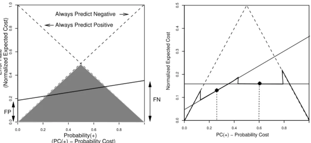
Estimates of the likelihoods are the false positive (FP) and false negative (FN) rates. A straight line, such as the one in bold in Figure 1, gives the error rate on the y-axis (ignore the axis labels in parentheses for the moment), for each possible prior probability of an instance belonging to the positive class on the x-axis. If this line is completely below another line, representing a second classifier, it has a lower error rate for every probability. If they cross, each classifier is better for some range of priors. Of particular note are the two trivial classifiers, the dashed lines in the figure. One always predicts that instances are negative, the other that instances are positive. Together they form the majority classifier, the shaded triangle in Figure 1, which predicts the most common class. The figure shows that any single classifier with a non-zero error rate will always be outperformed by the majority classifier if the priors are sufficiently skewed. It will therefore be of little use in this situation.

If misclassification costs are taken into account, expected error rate is re-placed by expected cost, defined by Equation 3. The expected cost is also a convex combination of the priors, but plotting it against them would produce a y-axis that no longer ranges from zero to one. The expected cost is normalized

(6)

0.6 0.0 0.2 0.4 0.6 0.8 0.0 0.2 0.8 1.0 0.4 Probability(+) (PC(+) − Probability Cost) FN Always Predict Positive

Always Predict Negative

(Normalized Expected Cost)

Error Rate

FP

Fig. 1.Majority Classifier

0.0 0.2 0.3 0.4 0.5 PC(+) − Probability Cost 0.0 0.2 0.4 0.6 0.8 0.1

Normalized Expected Cost

Fig. 2.The Cost Curve

by dividing by the maximum value, given by Equation 4. The costs and priors are combined into the P C(+) the Probability Cost on the x-axis, as in Equation 5. Applying the same normalization factor results in an x-axis that ranges from zero to one, as in Equation 6. The positive and negative Probability Costs now sum to one, as was the case with the probabilities.

E[Cost] = F N ∗ C(−|+)P (+) + F P ∗ C(+|−)P (−) (3) max(E[Cost]) = C(−|+)P (+) + C(+|−)P (−) (4) P C(+) = C(−|+)P (+) (5) N orm(E[Cost]) = F N ∗ P C(+) + F P ∗ P C(−) (6) With this representation, the axes in Figure 1 are simply relabeled, using the text in parentheses, to account for costs. Misclassification costs and class frequencies are more imbalanced the further away from 0.5, the center of the diagram. The lines are still straight. There is still a triangular shaded region, but now representing the classifier predicting the class with the smaller expected cost. For simplicity, we shall continue to refer to it as the majority classifier.

In Figure 2 the straight continuous lines are the expected cost for discrim-inative classifiers for two different class frequencies, or costs, indicated by the vertical dashed lines. To build a curve requires many different classifiers, each associated with the P C(+) value used to generate it. Let’s assume each classi-fier is used in the range from half way between its P C(+) value and that of its left neighbor to half way between this value and that of its right neighbor. The resulting black curve, which includes the trivial classifiers, is shown in Figure 2. It has discontinuities where the change over between classifiers occurs.

To produce a curve for a generative classifier, each instance is associated with the P C(+) value at which the classifier changes the way it is labeled. If the

(7)

instances are sorted according to this value, increasing P C(+) values generate unique F P and T P pairs. A curve is constructed in the same way as that for the discriminative classifiers. But now there are many more points, one for each instance in the test set, typically producing a much smoother looking curve.

4 Experiments

This section discusses experiments comparing the performance of various pop-ular algorithms, as implemented in the machine learning system called Weka [9]. The main set of experiments compares the expected cost of a single gen-erative classifier to that of a single discriminative classifier and to a series of such classifiers trained on data sets with different class frequencies. The ques-tion it addresses is to what extent the existing variants of standard algorithms are effective for cost sensitive learning. Further experiments look at how these probability estimators might be improved, firstly by calibration and secondly by using more balanced training sets.

To produce different P C(+) values, the training set is under-sampled, the number of instances of one class being reduced to produce the appropriate class distribution. This is done for 16 P C(+) values, roughly uniformly covering the range 0 to 1. The F P and T P values are estimated using ten-fold stratified cross validation. Experimental results, drawn from a larger experimental study [10], are given for 8 data sets from the UCI collection [11].

4.1 Decision Trees

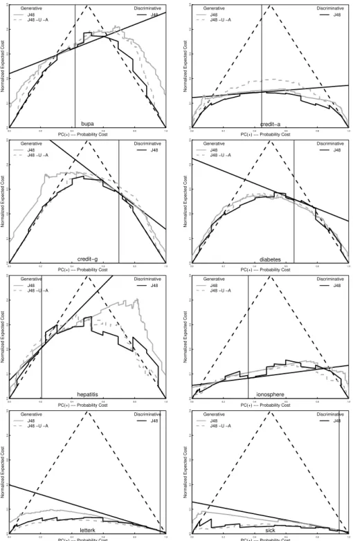
We begin with the decision tree algorithm J48, Weka’s version of C4.5 [12]. Figure 3 shows cost curves for the 8 data sets (the name is just above the x-axis). The gray solid curves give the expected cost for the generative classifier. This is calculated from probability estimates based on the class frequency at the leaves of the tree, adjusted for the class distribution in the training set.

To interpret these graphs, let us note that, in these experiments at least, there is little or no difference between discriminative and generative classifiers for the particular P C(+) value at which they were trained. The main advan-tage of a generative classifier is that it will operate effectively at a quite different P C(+) values. The solid black curve is for 14 discriminative classifiers generated by under-sampling. It acts, essentially, as a lower bound on the expected cost of using the generative classifier. The bold black straight line is the standard classifier trained (with default settings) at the original data set frequency, indi-cated by the vertical line. At this frequency, the black line, the gray solid curve, and the black curve have a similar expected cost (being essentially the same classifier). The cost sensitivity of the generative classifier is seen by comparing the distance of the gray curve to the straight black line and the distance to the black curve, as one moves away from the original frequency. Closer to the black curve is better.

(8)

0.0 0.2 0.4 0.6 0.8 1.0 0.0 0.1 0.2 0.3 0.4 0.5 PC(+) −− Probability Cost

bupa Generative J48 J48 −U −A Discriminative J48 0.0 0.2 0.4 0.6 0.8 1.0 0.0 0.1 0.2 0.3 0.4 0.5 PC(+) −− Probability Cost

credit−a Generative J48 J48 −U −A Discriminative J48 0.0 0.2 0.4 0.6 0.8 1.0 0.0 0.1 0.2 0.3 0.4 0.5 PC(+) −− Probability Cost

credit−g Generative J48 J48 −U −A Discriminative J48 0.0 0.2 0.4 0.6 0.8 1.0 0.0 0.1 0.2 0.3 0.4 0.5 PC(+) −− Probability Cost

diabetes Generative J48 J48 −U −A Discriminative J48 0.0 0.2 0.4 0.6 0.8 1.0 0.0 0.1 0.2 0.3 0.4 0.5 PC(+) −− Probability Cost

hepatitis Generative J48 J48 −U −A Discriminative J48 0.0 0.2 0.4 0.6 0.8 1.0 0.0 0.1 0.2 0.3 0.4 0.5 PC(+) −− Probability Cost

ionosphere Generative J48 J48 −U −A Discriminative J48 0.0 0.2 0.4 0.6 0.8 1.0 0.0 0.1 0.2 0.3 0.4 0.5 PC(+) −− Probability Cost

letterk Generative J48 J48 −U −A Discriminative J48 0.00.0 0.2 0.4 0.6 0.8 1.0 0.1 0.2 0.3 0.4 0.5 PC(+) −− Probability Cost

sick Generative J48 J48 −U −A Discriminative J48

(9)

bupa Original J48 −U −A Balanced J48 −U −A 0.00.0 0.2 0.4 0.6 0.8 1.0 0.1 0.2 0.3 0.4 0.5 PC(+) −− Probability Cost

hepatitis

Original J48 −U −A

Balanced J48 −U −A

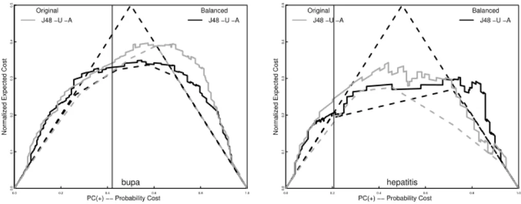
Fig. 4.Improving the Decision Tree Generative Classifier

Although close to the original frequency there is little to separate the curves, the difference grows as the distance increases. For P C(+) values closer to zero and one, the solid gray curves are much better than the single discriminative clas-sifiers and quite close to the multiple ones. Unfortunately, here the performance is worse than the majority classifier, making any gain over the discriminative classifier of dubious merit. One way to improve the probability estimates is to use Laplace correction at the leaves of an unpruned tree [6]. In Figure 3 this variant is indicated by the dashed gray curve. Generally, this improves on the standard algorithm, again it is most clear far away from the original frequency. For some data sets, e.g. letterK and Sick, it is indistinguishable from the black solid curve. But for other data sets, e.g. credit-a and hepatitis, without pruning means it is worse than the standard classifier around the original frequency.

There are two commonly methods to improve cost sensitivity: calibration and changing the training set distribution. Calibration refines the existing probability estimates to better reflect the true distribution using the training, or a hold-out, data. Figure 4 compares the cost curves to their lower envelopes, the dashed curves. The envelopes represent perfect calibration. The figure also shows results for using a balanced set for training the generative classifier. For many data sets, like Bupa and Hepatitis, balancing the training set makes the cost curve more symmetric. Calibration has greater potential impact, although often the best one might expect to do as well as the majority classifier far away from the original frequency.

4.2 Support Vector Machines

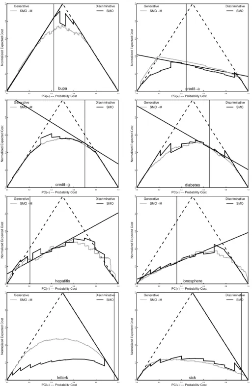
The original Support Vector Machine [2] had no means of producing probability estimates and only acted as a discriminative classifier. Platt [7] showed that a sigmoid could be applied to the normal output, the distance to the optimal hyperplane (the sign deciding the class), to represent the posterior probability. This sigmoid is learned from the training set (or by cross validation) using cross entropy as the error measure. Figure 5 shows that this variant, the gray curve,

(10)

bupa Generative SMO −M Discriminative SMO 0.0 0.2 0.4 0.6 0.8 1.0 0.0 0.1 0.2 0.3 0.4 0.5 PC(+) −− Probability Cost

credit−a Generative SMO −M Discriminative SMO 0.0 0.2 0.4 0.6 0.8 1.0 0.0 0.1 0.2 0.3 0.4 0.5 PC(+) −− Probability Cost

credit−g Generative SMO −M Discriminative SMO 0.0 0.2 0.4 0.6 0.8 1.0 0.0 0.1 0.2 0.3 0.4 0.5 PC(+) −− Probability Cost

diabetes Generative SMO −M Discriminative SMO 0.0 0.2 0.4 0.6 0.8 1.0 0.0 0.1 0.2 0.3 0.4 0.5 PC(+) −− Probability Cost

hepatitis Generative SMO −M Discriminative SMO 0.0 0.2 0.4 0.6 0.8 1.0 0.0 0.1 0.2 0.3 0.4 0.5 PC(+) −− Probability Cost

ionosphere Generative SMO −M Discriminative SMO 0.0 0.2 0.4 0.6 0.8 1.0 0.0 0.1 0.2 0.3 0.4 0.5 PC(+) −− Probability Cost

letterk Generative SMO −M Discriminative SMO 0.00.0 0.2 0.4 0.6 0.8 1.0 0.1 0.2 0.3 0.4 0.5 PC(+) −− Probability Cost

sick

Generative SMO −M

Discriminative SMO

(11)

letterk Original SMO −M Balanced SMO −M 0.00.0 0.2 0.4 0.6 0.8 1.0 0.1 0.2 0.3 0.4 0.5 PC(+) −− Probability Cost

credit−a

Original SMO −M

Balanced SMO −M

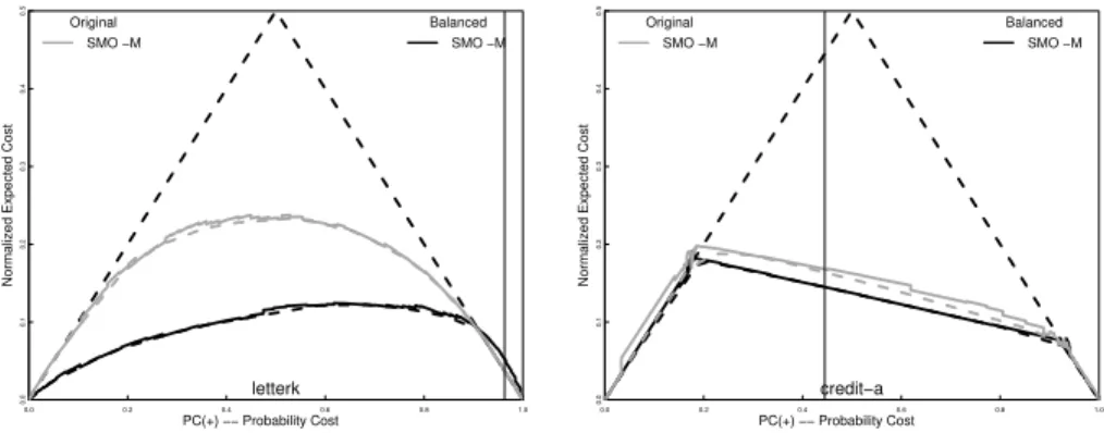
Fig. 6.Improving the Support Vector Machine Generative Classifier

is extremely competitive with the multiple discriminative classifiers. For only a couple of data sets, letterK and credit-a, are the two discernibly different.

Figure 6 shows, there is typically little difference between the cost curves (solid lines) and their lower envelopes (dashed lines), so calibrating the classifier should have little effect. This is not surprising as fitting a sigmoid is, itself, a form of calibration. Although the sigmoid only has two degrees of freedom, one can see more flexible schemes are unlikely to improve calibration much. This may be why no real benefit was seen using isotonic regression [13]. There is one data set, LetterK, that shows a large difference in expected cost. This is an extremely imbalanced domain and by training the classifier on a balanced data set, the black curves in Figure 6, considerable improvement is gained. For, credit-a the difference is smaller and largely on the left hand side of the original frequency. But here neither better balance nor calibration reduce the problem.

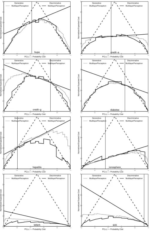
4.3 Neural Networks

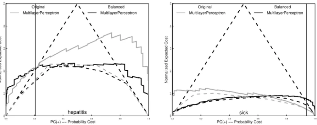
Weka implements the traditional PDP algorithm [14] which is trained using back propagation and minimizes the squared error of the network output. This can be used as a discrimination classifier or, by using the standard sigmoid output of the network, as a probability estimator. As Figure 7 shows, much like the standard decision tree, it improves on a single discriminative classifier but mainly where the majority classifier is best. It certainly falls way short of the performance of the multiple discriminative classifiers. Figure 8 shows that balancing the training set offers some improvement but much of the error is due to poor calibration. It is noteworthy that the Weka algorithm minimizes squared error. Minimizing cross entropy, like the generative version of the Support Vector Machine, should produce better probability estimates [15].

(12)

bupa Generative MultilayerPerceptron Discriminative MultilayerPerceptron 0.0 0.2 0.4 0.6 0.8 1.0 0.0 0.1 0.2 0.3 0.4 0.5 PC(+) −− Probability Cost

credit−a Generative MultilayerPerceptron Discriminative MultilayerPerceptron 0.0 0.2 0.4 0.6 0.8 1.0 0.0 0.1 0.2 0.3 0.4 0.5 PC(+) −− Probability Cost

credit−g Generative MultilayerPerceptron Discriminative MultilayerPerceptron 0.0 0.2 0.4 0.6 0.8 1.0 0.0 0.1 0.2 0.3 0.4 0.5 PC(+) −− Probability Cost

diabetes Generative MultilayerPerceptron Discriminative MultilayerPerceptron 0.0 0.2 0.4 0.6 0.8 1.0 0.0 0.1 0.2 0.3 0.4 0.5 PC(+) −− Probability Cost

hepatitis Generative MultilayerPerceptron Discriminative MultilayerPerceptron 0.0 0.2 0.4 0.6 0.8 1.0 0.0 0.1 0.2 0.3 0.4 0.5 PC(+) −− Probability Cost

ionosphere Generative MultilayerPerceptron Discriminative MultilayerPerceptron 0.0 0.2 0.4 0.6 0.8 1.0 0.0 0.1 0.2 0.3 0.4 0.5 PC(+) −− Probability Cost

letterk Generative MultilayerPerceptron Discriminative MultilayerPerceptron 0.00.0 0.2 0.4 0.6 0.8 1.0 0.1 0.2 0.3 0.4 0.5 PC(+) −− Probability Cost

sick

Generative MultilayerPerceptron

Discriminative MultilayerPerceptron

(13)

hepatitis Original MultilayerPerceptron Balanced MultilayerPerceptron 0.00.0 0.2 0.4 0.6 0.8 1.0 0.1 0.2 0.3 0.4 0.5 PC(+) −− Probability Cost

sick

Original MultilayerPerceptron

Balanced MultilayerPerceptron

Fig. 8.Improving the Multilayer Perceptron Generative Classifier

5 Discussion

In summary, the sigmoid variant for the Support Vector Machine, with a bal-anced training set, was extremely effective as a generative classifier. Decision trees with Laplace correction and, to lesser extent, the Multilayer Perceptron faired reasonably and both showed potential for improvement. Although balanc-ing is useful, calibration offers the most potential benefit and is notably inherent in the Support Vector Machine sigmoid fitting procedure.

In this paper, a curve made up of 16 discriminative classifiers has been used as a “gold standard”. A good generative classifier is assumed to be one whose performance is close to this “gold standard”. But to get good cost sensitive per-formance, one could simply use the 16 classifiers. The main advantage of the generative classifier is that it is a single classifier, reducing learning time and storage considerably. Another advantage is that a single classifier may be more understandable. Yet neither the Support Vector Machine nor the Multilayer Per-ceptron is easily understandable without extra processing. Even for the decision tree algorithm, as the generative version is unpruned, the classifier is more com-plex than any single discriminative classifier. It may be possible that a few, a lot less than the 16, judiciously chosen, discriminative classifiers would be very competitive. A tree with a stable splitting criterion but variable cost sensitive pruning [16] would have identical lower branches for all P C(+) values, making a collection of trees more easily understandable.

6 Conclusions

This paper experimentally compared the performance of discriminative and gen-erative classifiers for cost sensitive leaning. It showed that variants of commonly used algorithms produced reasonably effective generative classifiers. Where the classifiers were less effective, simple techniques like choosing the right training set distribution and calibration would improve their performance considerably.

(14)

References

1. Rubinstein, Y.D., Hastie, T.: Discriminative vs informative learning. In: Knowledge Discovery and Data Mining. (1997) 49–53

2. Vapnik, V.: Statistical Learning Theory. Wiley (1998)

3. Tong, S., Koller, D.: Restricted Bayes optimal classifiers. In: Proceedings of the 17th National Conference on Artificial Intelligence. (2000) 658–664

4. Ng, A.Y., Jordan, M.: On discriminative vs. generative classifiers: A comparison of logistic regression and naive Bayes. In: Advances in Neural Information Processing Systems 14. MIT Press (2002)

5. Jaakkola, T.S., Haussler, D.: Exploiting generative models in discriminative

classiers. In: Advances in Neural Information Processing Systems. MIT Press (1999) 487–493

6. Provost, F., Domingos, P.: Tree induction for probability-based ranking. Machine Learning 52 (2003)

7. Platt, J.: Probabilistic outputs for support vector machines and comparison to regularized likelihood methods. In: Advances in Large-Margin Classifiers. MIT Press (2000) 61–74

8. Drummond, C., Holte, R.C.: Cost curves: An improved method for visualizing classifier performance. Machine Learning (In Press)

9. Witten, I.H., Frank, E.: Data Mining: Practical machine learning tools and tech-niques. Morgan Kaufmann (2005)

10. Drummond, C.: Discriminative vs. generative classifiers: An in-depth experimen-tal comparison using cost curves. http://iit-iti.nrc-cnrc.gc.ca/personnel/

drummond_christopher_e.html(2006)

11. Blake, C.L., Merz, C.J.: UCI repository of machine learning databases. http: //www.ics.uci.edu/~mlearn/MLRepository.html (1998)

12. Quinlan, J.R.: C4.5 Programs for Machine Learning. Morgan Kaufmann (1993) 13. Zadrozny, B., Elkan, C.: Transforming classifier scores into accurate multiclass

probability estimates. In: Proceedings of the Eighth International Conference on Knowledge Discovery & Data Mining. (2002)

14. Rumelhart, D.E., McClelland, J.L.: Parallel distributed processing: explorations in the microstructure of cognition. MIT Press (1986)

15. Bishop, C.M.: Neural networks for pattern recognition. OUP (1996)

16. Drummond, C., Holte, R.C.: Exploiting the cost (in)sensitivity of decision tree splitting criteria. In: Proceedings of the 17th International Conference on Machine Learning. (2000) 239–246