Optimal Size of Nanoparticles for Magnetic Hyperthermia: A Combined Theoretical and Experimental Study

HAL Id: hal-01952258

https://hal.archives-ouvertes.fr/hal-01952258

HAL is a multi-disciplinary open access archive for the deposit and dissemination of sci-entific research documents, whether they are pub-lished or not. The documents may come from teaching and research institutions in France or abroad, or from public or private research centers.

L’archive ouverte pluridisciplinaire HAL, est destinée au dépôt et à la diffusion de documents scientifiques de niveau recherche, publiés ou non, émanant des établissements d’enseignement et de recherche français ou étrangers, des laboratoires publics ou privés.

Optimal Size of Nanoparticles for Magnetic

Hyperthermia: A Combined Theoretical and

Experimental Study

Boubker Mehdaoui, Anca Meffre, Julian Carrey, Sebastien Lachaize,

Lise-Marie Lacroix, Michel Gougeon, Bruno Chaudret, Marc Respaud

To cite this version:

Boubker Mehdaoui, Anca Meffre, Julian Carrey, Sebastien Lachaize, Lise-Marie Lacroix, et al.. Optimal Size of Nanoparticles for Magnetic Hyperthermia: A Combined Theoretical and Experimental Study. Advanced Functional Materials, Wiley, 2011, 21 (23), pp.4573-4581. �10.1002/adfm.201101243�. �hal-01952258�

DOI: 10.1002/adfm.((please insert DOI)

Optimal size of nanoparticles for magnetic hyperthermia: A combined theoretical and experimental study

By B. Mehdaoui, A. Meffre, J. Carrey*, S. Lachaize, L. M. Lacroix, M. Gougeon, B. Chaudret,

and M. Respaud

[*] Dr B. Mehdaoui, Dr A. Meffre, Dr J. Carrey Corresponding Author, Dr S. Lachaize, Dr L. M. Lacroix, Prof B. Chaudret, Prof M. Respaud

Université de Toulouse; INSA; UPS; LPCNO (Laboratoire de Physique et Chimie des Nano-Objets), 135 avenue de Rangueil, F-31077 Toulouse, France and

CNRS; UMR 5215 ; LPCNO, F-31077 Toulouse, France E-mail: (([email protected]))

Dr. M. Gougeon

Institut CARNOT - CIRIMAT - UMR 5085, Bâtiment 2R1, 118 route de Narbonne F-31062 Toulouse, France

Keywords: hyperthermia, magnetic nanoparticles, iron, hysteresis loop calculation

Progresses in the prediction and optimization of the heating of magnetic nanoparticles in an alternative magnetic field are highly desirable for their application in magnetic hyperthermia. Here a model system consisting of metallic iron nanoparticles with a size ranging from 5.5 to 28 nm is extensively studied. Different regimes as a function of the nanoparticles size are evidenced: single-domain superparamagnetic, single-domain ferromagnetic and multi-domain. Ferromagnetic single-domain nanoparticles are the best candidates and display the highest specific losses reported in the literature so far (11.2±1 mJ g-1_{). Measurements are analysed}

using state-of-the-art analytical formula and numerical simulations of hysteresis loops. Several features expected theoretically are observed for the first time experimentally: i) the correlation between the nanoparticle diameter and their coercive field ii) the correlation between the amplitude of the coercive field and the losses iii) the variation of the optimal size with the amplitude the magnetic field. None of these features are predicted by the linear response theory -generally used to interpret hyperthermia experiments- but are a natural

consequence of theories deriving from the Stoner-Wohlfarth model; they also appear clearly in numerical simulations. These results open the path to a more accurate description, prediction and analysis of magnetic hyperthermia.

1. Introduction

Magnetic hyperthermia (MH) is a promising therapeutic method based on the use of magnetic nanoparticles (MNPs). MH is a two step procedure: MNPs are first injected into the tumour; the patient is then immersed in an alternating magnetic field with a frequency f and an amplitude µ0Hmax appropriately chosen. Due to the excitation of the MNPs, the temperature

of the tumour rises

.

When applying an alternative magnetic field to MNPs, the area of their magnetic hysteresis loop A corresponds to a dissipated energy, which is used in MH. The power generated by the MNPs is evaluated by this specific area A (specific losses) or, more commonly used, by their specific absorption rate (SAR), the two parameters being linked by the equation SAR = Af. Exploiting this effect in oncology requires biocompatible MNPs with large heating power, thus one of the challenges in this topic is to maximize SAR values. The SAR being an increasing function of f and µ0Hmax, one could think of increasing these

parameters. However, human body cannot be exposed to alternating magnetic field of large

µ0Hmaxf product, due to medical limitation [7]. Therefore, optimizing the MNPs requires

optimizing their SAR at finite and specific values of the applied frequency and magnetic field. Typical values used in medical treatments so far are 100 kHz and 20 mT [8].

For experimentalists, there are three main ways to optimize the SAR. The first one is to increase the saturation magnetization MS of MNPs since the maximum SAR achievable is

directly proportional to MS. The second way is to optimize the anisotropy of the MNPs since

the importance of this parameter has been recently shown [9]. These first two points help in determining the optimal materials. Finally, for a given material, the next major parameter is the MNP size. An experimental study of this parameter requires synthesizing monodisperse MNPs with a varying mean size and studying the size-dependence of SAR. This has been realised in a few articles centred on the properties of iron oxide MNPs [10, 11, 12, 13, 14].

In the previous studies, when a quantitative analysis was tempted, [11, 12, 13, 14] the linear response theory (LRT) was always used, which is a major problem. Indeed, this theory has a restricted domain of validity [9], but the studies mentioned above have at some point used LRT out of this domain, which casts doubt on the results obtained (on this issue, see [ 15 ]). For a rigorous analysis of experimental data, theories derived from the Stoner-Wohlfarth model in their domain of validity should be used in complement to LRT [9, 16]. Out of the domain of validity of these two models, only numerical simulations can confidently calculate the SAR of single-domain MNPs [9, 17]. However, such simulations have never been applied so far for a direct comparison with experiments.

The aim of the present article is precisely to compare experiments performed on a model system consisting of Fe MNPs, with a tuneable mean size ranging from 5.5 to 28 nm, with state-of-the-art methods of analysis consisting of numerical simulations and adequate theories. Iron is a material with a weak anisotropy and a high MS; its magnetic properties are

less sensitive to unwanted size and surface effects such as dead layers than its oxide counterparts due to its metallic character. The synthesized Fe MNPs studied here are highly crystalline and display a MS value close to the bulk one in the whole range of size studied.

Thus, these MNPs constitute a perfect system for a fine study on the influence of the MNP size on MH.

Here we show that the magnetic-field dependence of the SAR and its amplitude strongly depends on the MNP size. In particular the specific losses are maximized for MNPs in a narrow range of diameters, and reach unprecedented values. Behaviour typical of single-domain MNPs in the superparamagnetic regime, in the ferromagnetic regime and of multi-domain MNPs are observed. Moreover, several features in the size-dependence of MH are reported here for the first time and can be well understood using theories derived from the Stoner-Wohlfarth model and numerical simulations. An original method for the quantitative analysis of MH is proposed and applied to our experimental results, permitting their fine analysis. Thus, this article confirms the limitation of LRT theory to explain experimental results on systems of interest for MH. It evidences that the use of suitable theories opens the path to more accurate description, prediction and analysis of MH.

2.1. Synthesis and characterisations

Our group has been investigating the elaboration of pure metallic iron(0) nanoparticles using an organometallic approach for about 10 years. [18, 19, 20] This approach is based on the decomposition of an iron source in a reductive medium in the presence of surfactants. By varying the reactants (iron source, surfactants) and the experimental conditions (concentration, temperature or pressure), we covered a large panel of size and shape for iron(0) nanoparticles. In this article, the iron sources were either the iron dimer {Fe[N(SiMe3)2]2}2 or the ultra-small Fe(0) NPs whose preparation has already been reported

elsewhere.[20] The surfactant system can be one of the two following combinations: palmitic acid (PA) / hexadecylamine (HDA) or hexadecylamonium chloride (HDA⋅HCl) / HDA. In all the cases, the reactants were reacted in mesitylen, under a reductive atmosphere of dihydrogen at 150°C for 2 days. Depending on the conditions, we forced different growth mechanisms to take place in order to change the morphology of the final NPs. Thus, the spherical NPs of samples 1 and 2 were formed thanks to an isotropic growth regulated by the PA/HDA ratio. Increasing the quantity of carboxylic acid over the amine led to a size increase because the growth is then favoured over the nucleation.[19] The same trend was observed for samples 3 to 7 that were prepared with the ammonium chloride HDA⋅HCl at various concentrations.[21] Samples 3 and 5 were prepared from the {Fe[N(SiMe3)2]2}2 iron source whereas samples 4, 6

and 7 were formed from ultra-small Fe(0) NPs. Changing the iron source nature helped us to produce different samples by playing with the different reduction kinetics. Tuning the experimental conditions finally allowed us to produce 7 samples of different shapes and mean sizes displaying a magnetization close to the bulk value. One main difference between the spherical and the cubic NPs is their aggregation in solution. Due to the shape and the larger mean size, the samples with cubic NPs are not colloids: the NPs self-organize into large superlattices. The latter are strongly stabilized by Van der Waals interactions between the alkyl chains of the surfactants at the surface of the NPs, and by magnetic interaction between the ferromagnetic NPs. These two contributions prevent any good dispersion of the NPs in compatible solvents.

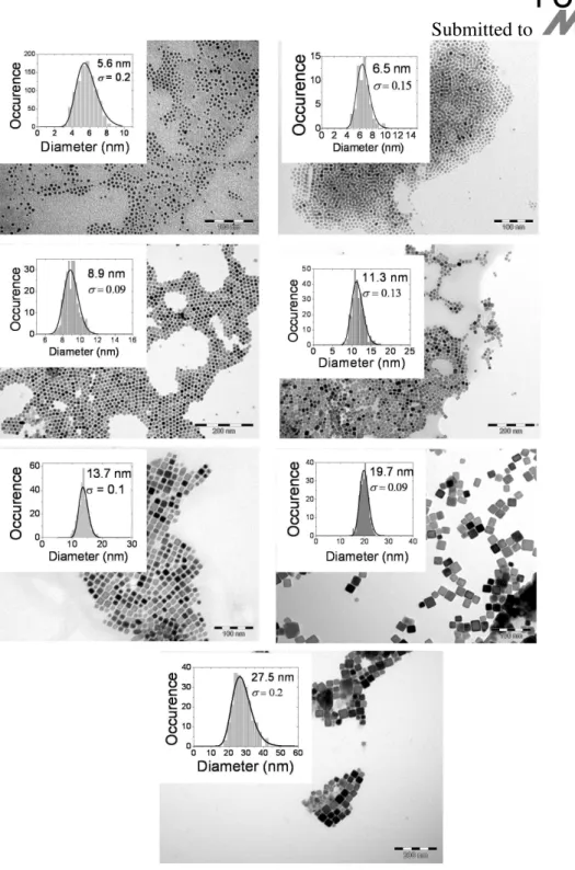
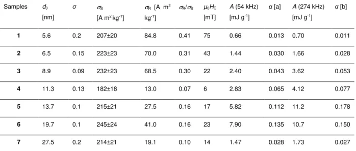
Transmission electron microscopy (TEM) characterisations of the samples are shown in Figure 1. Magnetic parameters extracted from SQUID measurements (see Supplementary Information) are summarized in Table 1. For all samples, except sample 4, the saturation magnetization per unit mass

σ

2.2. Magnetic hyperthermia measurements

MH measurements at 54 kHz were performed on a specially designed frequency-adjustable electromagnet [22]. This setup has been recently improved and allows us to work with a magnetic field up to µ0Hmax = 60 mT for frequencies f in the range 5-100 kHz.

Measurements at 274 kHz were performed using the coil of an induction oven, with a magnetic field up to µ0Hmax = 73 mT, similarly to experiments described in Ref. [23] (see

Experimental Section). Preliminary results on the MH properties of samples 1 and 4 were published in Refs [24] and [23], respectively.

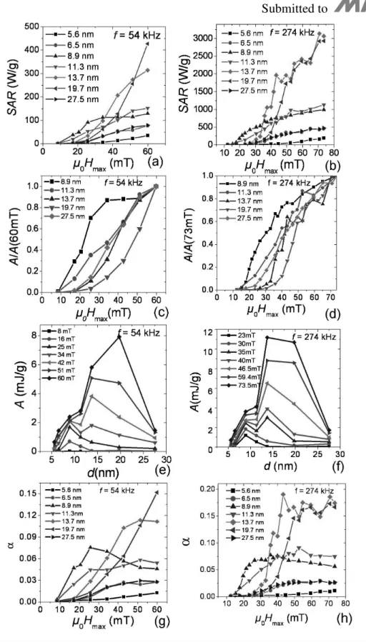
The SAR dependence as a function of magnetic field at frequencies f = 54 kHz and f = 274 kHz for samples 1-7 are shown in Figures 2a and 2b respectively. For sample 1 (d = 5.6 nm) the magnetic field dependence of the SAR follows a power law with an exponent of 2.8 and 3.1 at frequencies f = 54 kHz and 274 kHz respectively. Their behaviour has been analysed in details in a previous article and is typical of MNPs in the superparamagnetic regime [24].

In samples 3-7 (d = 8.9-27.5 nm), the SAR displays at 274 kHz a saturation at large magnetic field (see Figure 2b), which is typical of the ferromagnetic regime [16]. At 54 kHz, the saturation is only visible on sample 3 (d = 8.9 nm) because of the smaller maximum magnetic field available on this setup. On these samples the SAR shows a small amplitude at low magnetic field and a sharp increase above the coercive field of the MNPs, which is another feature of the ferromagnetic regime. The evolution of the coercive field with size is more clearly evidenced in Figure 2c and 2d, where the normalized SAR values are shown for these samples. In samples 3-6, the coercive field increases with the size of the MNPs. It can be observed that the amplitude of the SAR at large magnetic field is directly related to the amplitude of the coercive field : the larger the coercive field, the larger the SAR. In sample 7 (d = 27.5 nm), both the coercive field and the SAR displays an abrupt drop (see Figure 2a-d).

Another interesting way to plot the same experimental data is to display the size dependence of SAR for various applied magnetic fields. Such a plot is shown for the two frequencies in Figures 2e and 2f. It can be observed that, for each magnetic field, an optimal

diameter dopt maximizes the amplitude of SAR. Interestingly, dopt is not constant but increases

with the amplitude of the applied magnetic field.

Finally, the degree of optimization

α

f H

SAR =4αµ0 maxσS (1)

where σS is taken here as the bulk Fe value. α is a dimensionless parameter which

characterizes the relative area of the hysteresis loops with respect to the ideal square (α = 1). In Figures 2g and 2h the evolution of α as a function of the magnetic field and MNP diameter is shown and its value at saturation is summarized in Table I.

For a possible application of such nanoparticles in medical applications, the µ0Hmaxf

product is limited to be safe for the patient. We have performed hyperthermia measurements on the various samples at 35 kHz and 57 mT so as to keep the same µ0Hmaxf product as the

one currently used at the Charité Hospital [8]. The evolution of SAR, A and α with size are shown as Supporting Information. Sample 6 (d = 19.7 nm) displays the largest SAR = 290 W/g, corresponding to A = 8.3 mJ/g and α = 0.17.

A few comments on the data shown in Figure 2 can be made. First, the SAR values measured on the optimized samples are very large. At 54 kHz, the maximum SAR = 427±42 W g-1 occurs for sample 6 (d = 19.7 nm), while at f = 274 kHz, the maximum SAR = 3066±306 W g-1 _{occurs for sample 5 (d = 13.7 nm). In the latter case, this corresponds to}

specific losses A = 11.2±1 mJ g-1_{, which are the highest reported in the literature so far.}

Interestingly, large values of α are obtained only for values of the magnetic field greater than 50 mT. In a previous article, we had theoretically shown that iron MNPs -due to the value of their anisotropy field around 50 mT- should in principle be optimized nanoparticles only when magnetic fields of this order of magnitude are applied [9]. This is experimentally confirmed here. The largest α = 0.19 is observed in sample 5 (d = 13.7nm) under µ0Hmax = 43

from the maximum value achievable in a system with randomly oriented anisotropy axis α = 0.39 [9]. Thus our system could be optimized further, as will be discussed in Section 3.2.2.

3. Analysis

3.1 Qualitative analysis

3.1.1. Magnetic field dependence of SAR

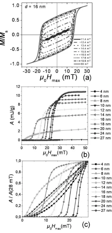
In this part, MH properties are calculated numerically without attempt to fit the experimental data. The results are then compared to experimental results for a qualitative analysis. The hysteresis loop area A is calculated for an assembly of spherical, uniaxial MNPs with their anisotropy axis randomly distributed in space, as detailed in Ref. [9]. The magnetic parameters of bulk iron have been used (MS = 1700 kA/m, the effective anisotropy Keff =

4.8×104 J m-3). The other parameters are T = 300 K, f = 100 kHz, and the frequency factor of the Néel-Brown relaxation time τ0 = 5×10-11 s As an illustration, the calculated hysteresis

loops for d = 16 nm are shown in Figure 3a as a function of the maximum field applied.

In Figure 3b the evolution of A with magnetic field for MNPs with a diameter d ranging from 4 nm to 24 nm is shown. In Figure 3c normalized data illustrating more clearly the evolution of the curve shape for the different diameters are shown. It can be seen that the shape of the A(µ0Hmax) evolves significantly with the diameter. For the smallest MNPs (d = 4

nm), A shows a square dependence with the magnetic field in agreement with LRT for superparamagnetic MNPs [9,25]. For sizes up to d =10 nm, A follows a power law, whose exponent vary with MNPs size [9]. For d ≥ 14 nm, the shape of the curves is characteristic of the ferromagnetic regime: the losses are very weak at low magnetic field followed by an increase around the coercive field and finally a progressive saturation [16,26].

The comparison between numerical calculations (Figure 3) and experiments (Figure 2) shows a qualitative agreement on three main features: i) the difference of behaviour between the superparamagnetic regime and the ferromagnetic one, the former displaying small SAR values and no saturation at large magnetic field, ii) the correlation between the amplitude of the coercive field and the amplitude of SAR for MNPs in the ferromagnetic regime and iii)

the increase of SAR with the MNP diameter at high magnetic field. The main point of discrepancy comes from the sample 7 (d = 27.5 nm), which displays an abrupt drop of coercive field and SAR. This drop in coercive field can be explained by the transition toward a multi-domain state of the MNP magnetization. Indeed, a transition from single-domain to vortex configuration has been calculated by micromagnetic simulations for Fe particles of roughly d = 26 nm [27]. Moreover, magnetic holography measurements performed on a 30 nm nanocube, similar to the ones composing this sample, have evidenced a vortex state of the magnetic configuration [28].

3.1.2. Optimal size

To study the optimal diameter dopt or the optimal volume Vopt for MH, the evolution of

A as a function of the diameter at a fixed µ0Hmax value must be evaluated. In order to do so,

hysteresis loops are calculated numerically for various sizes, the parameter values being chosen as previously. Figure 4a shows an example for µ0Hmax = 20 mT -which is the

magnetic field used during treatments [8]. For very small nanoparticles (d < dopt), the

hysteresis loop is almost reversible and specific losses A almost null, MNPs are superparamagnetic. When the volume increases, the hysteresis loop progressively opens and displays a typical ferromagnetic shape. The area of the hysteresis loop reaches a maximum for

d = dopt = 17.4 nm, plotted in thick line. For d > dopt, the coercive field is too large compared

to the applied magnetic field, so the magnetization of the MNPs cannot be switched, leading to minor loops only. Thus, the losses decrease with increasing size, and vanish at very large size.

The evolution of the area A as a function of the MNP size is summarized in Figure 4b for various magnetic field amplitudes. The presence of an optimal diameter is clearly visible, permitting to plot the evolution of dopt as a function of the magnetic field (Figure 4c). At very

low magnetic field amplitude, the optimal diameter dopt =11.7 nm is independent of the

magnetic field amplitude. With strengthened µ0Hmax, dopt increases. The optimal size, derived

here above from numerical calculations, can also be predicted analytically using two models. At low field, for µ0Hmax < 2.7 mT, LRT is valid, so the optimum volume is given by the

following equation [9]: ) ln(πfτ₀ K T k V B opt = (2)

The optimal volume is thus constant at low field, as represented in Figure 4c by the horizontal solid line.

In the ferromagnetic regime, LRT is no more valid, therefore theories derived from the Stoner-Wohlfarth model should be used instead. In this framework, one can have access to the optimal volume through the optimization of the coercive field µ0HC which reads [9]:

), 1 ( 48 . 0 ₀ 0.8 0HC = µ HK −κ µ (3) where S K M K

H = 2 is the anisotropy field and

. 4 ln 0 max 0       =

τ

κ

Note that Equation (3) is only valid when κ < 0.7. The maximum value for A is obtained for an optimal coercive field, the value of which is slightly below the applied magnetic field [6] :

(

)

0H µ H

µ _C = ± (5)

Using Equations (3) and (5), one can then deduce the optimal volume and thus, the optimal diameter. The result of this resolution is shown in Figure 4c as a dashed line in the domain of validity of Equation (3). This figure illustrates that the evolution of the optimal size at large magnetic field is a natural consequence of theories derived from the Stoner-Wohlfarth model.

Here again, comparing Figure 4b with Figure 2e-f shows that this feature is observed experimentally, since the optimal diameter increases with the magnetic field. This evolution comes with an increase of SAR. This is the first time that this feature is observed experimentally.

3.2 Quantitative analysis

3.2.1. Method and hypothesis

The experimental and theoretical results presented above are in good qualitative agreement, insofar as all the main features predicted theoretically are observed experimentally. However, there are some quantitative disagreements on the values of the losses, on the optimal diameters and on the coercive field values. These differences cannot be explained only by the frequency used. For instance, a coercive field of ca. 10 mT is

determined numerically for 14nm MNPs at 100 kHz (cf Figure 3b) while values of ca. 40 and 35 mT are respectively obtained at 54 and 274 kHz (cf Figure 2c-d). This discrepancy might result from several effects: different values of τ0 and/or Keff, influence of size distribution

and/or of magnetic interactions. In order to determine the origin of this discrepancy, a quantitative analysis of the experimental results is required.

Due to the fact that the calculation time of a typical graph in Figures 3 or 4 is around one week, it is not reasonable to expect to vary both τ0 and Keff in numerical simulations until

a good fit of experimental data is achieved. To make a quantitative analysis possible, a special method must be used and a few assumptions made. The method is the following: i) a “coercive field value deduced from MH experiments” µ₀H_CHyp is defined as the point of highest slope in SAR(µ0Hmax) functions. The interest of µ₀H_CHyp is that it can be calculated

analytically for a sample composed of single-domain MNPs in the ferromagnetic regime. ii) Thus our analysis is restricted to the samples 3-6 (d = 8.9-19.7 nm), given that these samples match these requirements. iii) We assume that these four samples have the same Keff value,

which it is not unreasonable since surface effects are limited in this size range, and have also the same τ0 value. iv) The evolution of µ₀H_CHyp with diameter is fitted analytically to

determine τ0 and Keff. v) These two parameters are then injected into numerical simulations to

obtain the complete and exact SAR values.

The calculation of µ₀H_CHyp as a function of the experimental parameters requires solving numerically:                         − = 8 . 0 0 0 0 0 4 ln 1 463 . 0 τ Vf M H µ T k V K T k H µ H µ S CHyp B eff B K CHyp (6)

Details on the origin and domain of validity of this equation can be found in Supporting Information.

3.2.2. Results

The quantitative analysis of the data has been performed for measurements at 55 and at 274 kHz and lead to compatible results. We will focus here on the results obtained at 274

kHz, provided that the values of µ0HCHyp have a lower error bar due to the higher range of

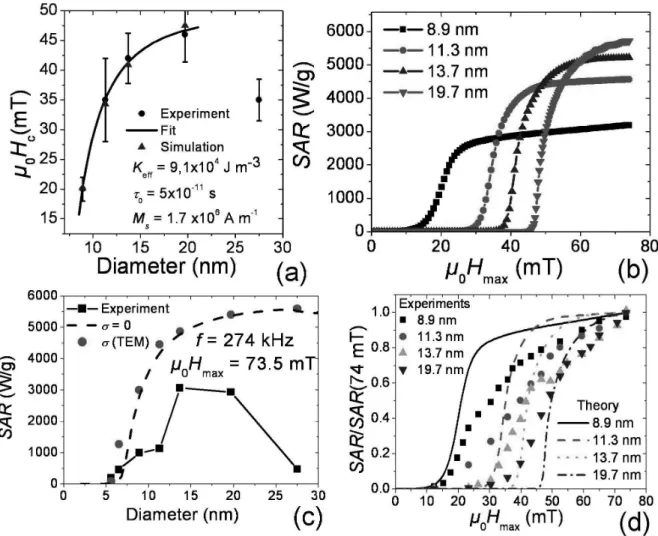
magnetic field used. In Figure 5a, the coercive field µ0HCHyp deduced from the highest slope

of the SAR(µ0Hmax) function is displayed for the four samples. The value for the sample 7 (d

= 27.5 nm) is also shown for indication but is not taken into account in the quantitative analysis due to its multi-domain configuration. The size evolution of the coercive field is fitted using Equation (6) with τ0 and Keff as varying parameters and σS = 212 A m2 kg-1, T =

300 K and f = 274 kHz. The best fit of experimental data is obtained for Keff = 9.1×104 J m-3

and τ0 = 5×10-11 s (see Figure 5a). These values have a correct order of magnitude, though τ0

is smaller than the values usually reported for individual MNPs (10-9 _{– 10}-10 _{s) and K} eff

slightly larger than the bulk value. These values were used for numerical simulations and the results compared with experimental data. In Figure 5b, the numerically calculated SAR obtained for the four samples using these parameters are shown. The coercive fields extracted from these curves are shown in Figure 5a as triangles: the points of maximum slope in numerically calculated SAR(µ0Hmax) matches the experimental points highlighting the

coherency of our method.

The first point of discrepancy between theory and experiments is the amplitude of the SAR. Experimental values as a function of the diameter SAR(d) are plotted in Figure 5c as square points. Theoretical SAR values, plotted as a dashed line, are well above the experimental values, this for all four samples investigated. To check if this higher value arises from the influence of the size distribution of MNPs, the calculated SAR(d) function is convoluted with the size distribution deduced from TEM images and plotted as circles in Figure 5c. For large MNPs, the size distribution has a negligible influence, while for small MNPs, the size distribution increases the SAR values. Thus, the size distribution effect can not be held responsible for the smaller experimental SAR values.

Another hypothesis to explain the discrepancy between theory and experiments is the presence of magnetic interactions in the samples whereas the simulations assume non-interacting nanoparticles. In a recent article, D. Serantes et al., have found using numerical simulations of interacting MNPs that ferromagnetic MNPs in dipolar interactions display an enhanced (reduced) SAR at low (high) field, and saturate at a higher field than independent MNPs [ 29 ]. For a better comparison on the shape of experimental and theoretical

from the samples 4-6 (d = 11.3-19.7 nm) show a striking similarity with the theoretical curves published by D. Serantes et al. As a consequence, we attribute the discrepancies between numerical simulations and experimental data to the presence of magnetic interactions in our samples leading to reduced SAR values and enlarged step width in the SAR(µ0Hmax) function

around the coercive field. This would explain that, even in our optimized samples, α value does not reach the highest possible value (see section 2.2). The next step of optimization would thus consist in elaborating magnetically independent ferromagnetic MNPs of optimized diameter.

4. Conclusions

Extensive MH measurements have been performed on a model system consisting of iron MNPs in a size range going from 5.5 to 27.5 nm. The results have been analysed using state-of-the-art numerical simulations of hysteresis loops and analytical formula. Several features theoretically predicted have been observed for the first time in MH experiments: i) the increase of coercive field with the size of MNPs ii) the correlation between the amplitude of the coercive field and the amplitude of the SAR iii) the fact that the optimal size depends on the amplitude of the magnetic field. None of these features are predicted by the LRT, though this is the theory that has been the most used so far in MH. These features are however a natural consequence of theories deriving from the Stoner-Wohlfarth model and also appear clearly in numerical simulations. Furthermore the transition toward multi-domain MNPs is clearly detected experimentally by an abrupt drop of both coercive field and SAR, confirming that such MNPs are not the most efficient for MH, the optimized objects being single-domain MNPs.

The variation of coercive field with the diameter of the MNPs is quantitatively reproduced by a simple model of monodisperse non-interacting single-domain MNPs with size-independent τ0 and Keff values. However, such a model does not correctly reproduce the

amplitude of the SAR and its magnetic field dependence. The quantitative analysis we have performed shows that this discrepancy is not due to the effect of size distribution but more likely to the effect of magnetic interactions.

Iron MNPs with optimized properties display hysteresis area values A = 11±1 mJ g-1 at

µ0Hmax = 73 mT, which is the highest value of the literature so far. The study of their α

parameter has shown that they reveal their potential only when large magnetic fields are applied. Keeping a µ0Hmaxf product similar to the one used during MH treatments, they

display a SAR of 290 W g-1. We have seen that this value could be further enhanced since α and thus the SAR could be multiplied by a factor between 3 and 7. The next step of our study will be to reduce the importance of magnetic interactions in our system to check if MH experiments and numerical simulations would be in quantitative agreement in system of non-interacting MNPs.

Once protected from oxidation, these high-magnetization nano-objects could be useful for several biomedical applications besides magnetic hyperthermia, such as magnetic labelling, drug targeting or contrast enhancement in MRI [30]. For this purpose, a silica layer can be used, as recently patented by our group [31]; this layer could also ensure an easy functionalization of the objects. However, the question of their eventual toxicity should unquestionably be addressed.

5. Experimental

Nanoparticles synthesis : All the preparations and syntheses are performed under either an

inert atmosphere of argon or a reductive atmosphere of hydrogen using a glove-box and Fisher-Porter bottles. Mesitylene (99%, VWR Prolabo) was dried over alumina and degassed by three pump-freeze-thaw cycles. Hexadecylamine (HAD, 99%, Aldrich) was used without purification. Hexadecylammonium chloride was prepared according to published procedure. [32] The {Fe[N(SiMe3)2]2}2 dimer was brought to NanoMePS and used as-received.

Ultra-small iron(0) NPs were prepared according to published procedure [20].

Synthesis of samples 1 and 2: A solution of palmitic acid (256 mg, 1 mmol for sample 1 and

358 mg, 1,4 mmols for sample 2; 384 mg, 1.5 mmols) in mesitylene (5 ml) was added to a green solution of {Fe[N(SiMe3)2]2}2 (376.5 mg, 0.5 mmol) in mesitylene (10 ml) in a Ficher

Porter bottle. A solution of hexadecylamine (483 mg, 2 mmols) in mesitylene (5 ml) was then added to this mixture. Its color turned to black. The reacting medium was pressurized under 3 bars dihydrogen then heated at 150°C for 48 hours. Excess dihydrogen was evacuated and the solution was let to cool at room temperature. The magnetically collected black powder was washed three times with toluene (15 ml). It yielded a material that contained xx% and 24.1% of iron in samples 1 and 2 respectively.

Synthesis of samples 3 and 4: Hexadecylamonium chloride (277 mg, 1 mmol and 415,5 mg,

1,5 mmols) was added to a green solution of {Fe[N(SiMe3)2]2}2 (376,5 mg, 0.5 mmol) in

mesitylene (15 ml) in a Ficher Porter bottle. The color changed immediately from green to yellow. A solution of hexadecylamine (483 mg, 2 mmols in both cases) in mesitylene (5 ml) was then added to this mixture. Its color turned to black. The reacting medium was heated at 90°C for 30 minutes, cooled down to room temperature, then pressurized under 3 bars dihydrogen and heated again at 150°C for 48 hours. Excess dihydrogen was evacuated and the solution was let to cool down at room temperature. The magnetically collected black powder was washed three times with toluene (15 ml). It yielded a material that contained 70.4% and 68.8% of iron for samples 3 and 4 respectively.

Synthesis of samples 5, 6 and 7: Ultra-small iron NPs (1 mmol of Fe) were prepared in 10 mL

of mesitylene. Hexadecylammonium chloride (304,5 mg, 1.1 mmols for 5; 277 mg, 1 mmol for 6; 554 mg, 2 mmols for 7) and hexadecylamine (483 mg, 2 mmols in the three cases) were successively added to the NPs solution. The reacting medium was heated at 90°C for 30 minutes, cooled to room temperature, pressurized under 3 bars dihydrogen and then heated again at 150°C for 48 hours. Excess dihydrogen was evacuated and the solution was let to cool down at room temperature. The magnetically collected black powder was washed three times with toluene (15 ml). It yielded a material that contained 81.1%, 75.6% and 91.2% of iron in samples 5, 6 and 7 respectively.

Magnetic measurements: The magnetization and the coercive field of as-synthesized iron(0)

NPs were measured on a Quantum Design Model MPMS 5.5 SQUID magnetometer. The absolute magnetization was deduced from the iron(0) total content determined by Inductively Coupled Plasma – Mass Spectrometry. These studies were carried out on powder samples that were prepared and sealed under an argon atmosphere to preserve the metallic character of iron. Extreme care was taken to avoid oxidation during the transfer to the apparatus.

Hyperthermia measurements: For hyperthermia measurements, a schlenk containing about 12

mg of powder of Fe NPs and 0.5 ml of mesitylene was filled under inert atmosphere to prevent any oxidation of the NPs. The mesitylene was used as solvent to ensure the solubility of the nanoparticles and because of his high boiling point. The schlenk is then placed in a calorimeter with 1.5 ml of deionised water, the temperature of which was measured. The measurement time was varied between 30 and 100 s, depending on the experimental

parameters, so that the temperature rise never exceeds 20°C. The temperature rise at the end of the magnetic field application was always measured after shaking the calorimeter to ensure the temperature homogeneity, which was checked by putting two probes at the top and the bottom of the calorimeter. The temperature rise is determined after this process from the mean slope of the ∆T/∆t function. Then the SAR values were calculated using the expression:

t T m m C SAR Fe i i pi ∆ ∆ =

∑

Where Cpi and mi are specific heat capacity and mass for each component (Cp = 449 J kg-1K-1

for Fe NPs, Cp = 1750 J kg-1K-1 for mesitylene, Cp = 4186 J kg-1K-1 for water and Cp = 720 J

kg-1K-1 for glass), and mFe is the mass of the pure Fe MNPs. The mass of glass is put to 2930

mg. Dividing SAR values by the magnetic field frequency lead to the specific losses A.

Acknowledgements

This work was supported by the InNaBioSanté Foundation. Supporting Information is available online from Wiley InterScience or from the author.

Received: ((will be filled in by the editorial staff)) Revised: ((will be filled in by the editorial staff)) Published online: ((will be filled in by the editorial staff))

_[1] P. Moroz, S. K. Jones, and B. N. Gray, Int, J. Hyperthermia 2002 18, 267. _[2] J. J. W. Lagendijk, Phys. Med. Biol. 2000, 45, R61.

_[3] A. Jordan, R. Scholz, K. Maier-Hauff, M. Johannsen, P. Wust, J. Nadobny, H. Schirra, H. Schmidt, S. Deger, S. Loening, W. Lanksch, R. Felix, J. Magn. Magn. Mater. 2001, 225, 118.

_[4] K. Maier-Hauff, R. Rothe, R. Scholz, U. Gneveckow, P. Wust, B. Thiesen, A. Feussner, A. von Deimling, N. Waldoefner, R. Felix and A. Jordan, J Neurooncol 2007 81, 53

_[5] K. Maier-Hauff, F. Ulrich, D. Nestler, H. Niehoff, P. Wust, B. Thiesen, H. Orawa,V. Budach and A. Jordan, J. Neurooncol. 2011 103, 317

_[6] M. Johannsen, U. Gneveckow, B. Thiesen, K. Taymoorian, C. H. Cho, N. Waldöfner, R. Scholz, A. Jordan, S. A. Loening, P. Wust, European Urology 2007 52, 1653

_[7] I.A. Brezovich, Med. Phys. Monogr. 1988, 16, 82.

_[8] P. Wust, U. Gneveckow, M. Johannsen, D. Böhmer, T. Henkel, F. Kahmann, J. Sehouli, R. Felix, J. Ricke, A. Jordan, Int. J. Hyperthermia 2006 22, 673.

_[9] J. Carrey, B. Mehdaoui, M. Respaud, J. Appl. Phys. 2011, 109, 083921

_[10] R. Hergt, R. Hiergeist, M. Zeisberger, G. Glöckl, W. Weitschies, L.P. Ramirez, I. Hilger and W.A. Kaiser, J. Magn. Magn. Mater. 2004, 280, 358.

_[11] J.-P. Fortin, C. Wilhelm, J. Servais, C. Ménager, J.-C. Bacri and F. Gazeau, J. Am.

Chem. Soc. 2007, 129, 2628.

_[12] M. Lévy, C. Wilhelm, J-M. Siaugue, O. Horner, J-C. Bacri and F. Gazeau, J. Phys.:

Condens. Mater. 2008, 20, 204133.

_[ 13 ] G. F. Goya, E. Lima, A. D. Arelaro, T. Torres, H. R. Rechenberg, L. Rossi, C. Marquina and M. R. Ibarra, IEEE Trans. Magn. 2008, 44, 4444.

_[14] M. Gonzales-Weimuller, M. Zeisberger, K. M. Krishnan, J. Magn. Magn. Mater. 2009, 321, 1947.

_[15] R. Hergt, S. Dutz and M. Zeisberger, Nanotechnology 2010, 21, 015706.

_[16] L.-M. Lacroix, R. Bel-Malaki, J. Carrey, S. Lachaize, G. F. Goya, B. Chaudret, M. Respaud, J. Appl. Phys. 2009, 105, 023911.

_[17] N. A. Usov, J. Appl. Phys. 2010, 107, 123909.

_[18] F. Dumestre, B. Chaudret, C. Amiens, P. Renaud, and P. Fejes, Science 2004, 303, 821. _[19] L.-M. Lacroix, S. Lachaize, A. Falqui, M. Respaud, and B. Chaudret, J. Am. Chem. Soc. 2009, 131, 549.

_[20] L.-M. Lacroix, S. Lachaize, A. Falqui, T. Blon, J. Carrey, and M. Respaud, F.

Dumestre, C. Amiens, O. Margeat, and B. Chaudret, P. Lecante and E. Snoeck, J. Appl. Phys. 2008, 103, 07D521.

_[21] A. Meffre, S. Lachaize, M. Respaud, B. Chaudret, in preparation

_[22] L.-M. Lacroix, J. Carrey, and M. Respaud, Rev. Sci. Instrum.2008, 79, 093909.

_[23] B. Mehdaoui, A. Meffre, L. M. Lacroix, J. Carrey, S. Lachaize, M. Goujeon, M. Respaud, B. Chaudret, J. Magn. Magn. Mater. 2010, 322, L49.

_[24] B. Mehdaoui, A. Meffre, L. M. Lacroix, J. Carrey, S. Lachaize, M. Goujeon, M. Respaud, B. Chaudret, J. Appl. Phys. 2010, 107, 09A324.

_[25] R. E. Rosensweig, J. Magn. Magn. Mater. 2002, 252, 370.

_[26] Y. L. Raikher, V. I. Stepanov, R. Perzynski, Physica B 2004, 343, 262. _[27] W. Rave, K. Fanian, A. Hubert, J. Magn. Magn. Mater. 1998, 190, 332.

_[28] E. Snoeck, C. Gatel, L.M. Lacroix, T. Blon, S. Lachaize, J. Carrey, M. Respaud, B. Chaudret, Nanoletters 2008, 8, 4293

_[29] D. Serantes, D. Baldomir, C. Martinez-Boubeta, K. Simeonidis, M. Angelakeris, E. Natividad, M. Castro, A. Mediano, D.-X. Chen, A. Sanchez, LI. Balcells and B. Martínez, J.

Appl. Phys. 2010, 108, 073918.

_[30] Q. A. Pankhurst, J. Connolly, S. K. Jones and J Dobson, J. Phys. D: Appl. Phys. 2003, 36 R167–R181

_[31] F. Delpech, C. Nayral, N. El Hawi, WO/2009/071794

_[32] K. Soulantika, A. Maisonnat, M.-C. Fromen, M.-J. Casanove, B. Chaudret, Angew.

Figure 1. Transmission electron microscopy image of the different samples and

corresponding size distribution. The histogram was fitted with a log-normal distribution to estimate the mean particle size d0 and the standard deviation σ.

Figure 2. Hyperthermia measurement at frequency f = 54 kHz (left) and f = 274 kHz (right). (a) and (b) Evolution of the SAR as a function of magnetic field for different samples. (c) and (d) Normalized SAR value for NPs ranging between 8.9 and 27.5 nm. (e) and (f) Size

dependence of SAR at different magnetic fields. (g) and (h) Data of (a) and (b) modified using Equation (1) to plot the magnetic field dependence of α.

Figure 3. Numerical simulations of the hysteresis area using the parameters of bulk iron. Keff

= 4.8×104 _{J m}-3_, τ

0 = 5×10-11 s, MS = 1.7 kA m-1, T = 300 K, f =100 kHz. (a) Evolution of the

hysteresis loops as a function of the magnetic field for d = 16 nm. (b) Evolution of area as a function of magnetic field for different sizes. (c) Normalized hysteresis area for different size.

Figure 4. (a) Evolution of the hysteresis loop as a function of size for µ0Hmax = 20 mT. (b)

Evolution of hysteresis area as a function of size NPs at different magnetic field. (c)

Comparison between the optimal diameters calculated analytically using Equation (2) (solid line), Equations (3), (4), (5) (dashed line) , and the ones extracted from numerical simulations (star points).

Figure 5. Quantitative analysis of data at f = 274 kHz (a) Evolution of µ0HCHyp determined

from experiments (round dots), from a fit using Equation (6) (solid line), and from the

numerical simulations (triangles). Ms = 1.7×106 A m-1, T = 300 K, f = 274 kHz, τ0 = 5×10-11 s

and Keff = 9.1×104 J m-3. (b) SAR (µ0Hmax) calculated numerically for four diameters using

these parameters. (c) Numerical calculations of the SAR at µ0Hmax = 73.5 mT as a function of

the diameter when neglecting the effect of size distribution (dashed line), or using the size distribution deduced from TEM (round dots). Corresponding experimental values (square points). (d) Normalized SAR (µ0Hmax). Dots represents experimental values and lines are

Table 1. Summary of magnetic and hyperthermia properties of the different samples: mean diameter d0, standard deviation σ, saturation magnetization σS, remnant magnetization σR,

ratio σR / σS, coercive field µ0HC, losses per cycle A at f = 54 kHz, 60 mT, and at f = 274 kHz,

73 mT, and corresponding α values calculated using Equation (1).

Samples d0 [nm] σ σS [A m2 _kg-1_] σR [A m2 kg-1_] σR/σS µ0HC [mT] A (54 kHz) [mJ g-1 ] α _[a] A (274 kHz) [mJ g-1 ] α _[b] 1 _{5.6 0.2 207±20 84.8 0.41 75 0.66 0.013 0.70 0.011} 2 _{6.5 0.15 223±23 70.0 0.31 43 1.44 0.030 1.66 0.028} 3 _{8.9 0.09 232±23 68.5 0.30 22 2.40 0.043 3.62 0.053} 4 _{11.3 0.13 182±18 13.0 0.07 6 2.83 0.065 4.12 0.077} 5 _{13.7 0.1 215±21 27.5 0.16 17 5.82 0.112 11.2 0.178} 6 _{19.7 0.1 245±24 41.0 0.16 23 7.90 0.135 10.7 0.150} 7 _{27.5 0.2 214±21 19.1 0.10 14 1.47 0.028 1.73 0.027}

[a] α values for measurements at µ0Hmax = 60 mT and f = 54 kHz.

The table of contents entry should be fifty to sixty words long, written in the present tense, and refer to the chosen figure.

Magnetic Nanoparticles, Biomedical Applications, Fe Nanoparticles

By B. Mehdaoui, A. Meffre, J. Carrey*, S. Lachaize, L. M. Lacroix, M. Gougeon, B. Chaudret ,and M. Respaud

Optimal size of nanoparticles for magnetic hyperthermia: A combined theoretical and experimental study

ToC figure ((Please choose one size: 55 mm broad × 50 mm high or 110 mm broad × 20 mm high. Please do not use any other dimensions))

Heating power of metallic iron magnetic nanoparticles whose diameter ranges from 5.5 nm to 28 nm is measured in an alternative applied magnetic field of frequency of 54 kHz and of amplitude ranging from 8 to 60 mT. The optimal size is visible as a maximum in the curve. Optimized nanoparticles display losses of 8 mJ g-1 _{at this frequency.}