Boundary layer and shock detection in CFD solutions

Boundary Layer and Shock Detection in CFD

Solutions

by

David Lovely

Submitted to the Department of Aeronautics and Astronautics

in partial fulfillment of the requirements for the degree of

Masters of Science in Aeronautical Engineering

at the

MASSACHUSETTS INSTITUTE OF TECHNOLOGY

February 2000

©

Massachusetts Institute of Technology 2000. All rights reserved.

A uthor ... ....

...

Department of Xeronautics and Astronautics

October 18, 1999

C ertified by ...

Robert Haimes

Principal Research Engineer

Thesis Supervisor

Accepted by ...

SEP 0 7 2000

Nesbitt Hagood

Boundary Layer and Shock Detection in CFD Solutions

by

David Lovely

Submitted to the Department of Aeronautics and Astronautics on October 18, 1999, in partial fulfillment of the

requirements for the degree of

Masters of Science in Aeronautical Engineering

Abstract

The motivation for feature detection research is to provide analysts with quantitative information about features of interest, without the need for manually probing the solution field. This thesis investigates new feature detection algorithms for shocks in compressible flow solutions and boundary layers in viscous solutions. These new algorithms were designed to be applied in a co-processing step, filtering the massive quantities of data and extracting physically meaningful flow characteristics.

Shock detection algorithms were developed to locate, classify and determine shock strength for both transient and steady state solutions. The algorithm uses the physics of the flow field to calculate a marker quantity that correlates with the location of shock. The marker quantity is an approximation to the Mach number normal to a moving or stationary shock. Since the Mach number relative to the shock wave has to pass through unity, this number can be used as a threshold to mark regions of likely shocks. Unfortunately, the marker quantity has some undesirable properties for a shock detector, picking out areas of the flow that are not shocks, so some other filters had to be created to remove these false indications.

The boundary layer algorithms estimate the displacement and momentum thick-ness on the solid boundaries of a CFD solution domain. The challenge in designing this algorithm was to make it applicable to any geometry and flow situation. This required a careful definition of the boundary layer, because some measures of the boundary layer thickness have a physical meaning in the two-dimensional flows, but loose that meaning in moving to a more complex topology.

The boundary layer thickness algorithms works in two steps, first estimating the free stream velocity by integrating vorticity components along curves normal to the wall. The second step is to integrate the mass flow rate and momentum flow rate in this region and construct a displacement and momentum thickness from these quantities. Comparisons were made between the actual free stream velocities and calculated free stream velocities for some standard two and three-dimensional flows. Results were encouraging; often coming within a percentage of the theoretical value,

culations. The technique involves casting the streamline and stream-tube integrations as a linear convection problem, and then solving that problem. Results of the full boundary layer thickness estimation technique applied to a corner flow model show that it is possible to estimate the boundary layer thickness as a function along the solid surface of the model, without having any discontinuities in the function. The technique was also tested on two airfoil flow models, one in a laminar flow regime, the other in a turbulent flow. The comparison of displacement thickness estimated with the new technique to the displacement thickness calculated within the CFD solution process was within 10 percent.

Applications to more complex flows will have to deal with cases where vorticity is added from outside the boundary layer such as curved shocks and wakes from upstream bodies, but do not effect boundary layer thickness.

Thesis Supervisor: Robert Haimes Title: Principal Research Engineer

Acknowledgments

The shock detection algorithm has been an extension of the work done by David Darmofal and others. Professor Mark Drela was instrumental in finding the unsteady extensions to the basic algorithm, as well as providing understanding of the boundary layer equations. Tim Barth was also a great resource for discussing boundary layer detection. I would also like to thank others in the Fluid Dyamics Research Lab, Ali Merchant and Alex Budge in particular for letting me use there datasets.

Funding for this project has been provided by NASA Ames, through grant number

0.1

Shock Wave Nomenclature

P

ratio of specific heats

qf Velocity

0.2

Boundary Layer Nomenclature

P Pressure

p Density

6 boundary-layer thickness

61 Displacement thickness

62 Momentum thickness

U Velocity outside the boundary layer u local x velocity component

v local y velocity component w local z velocity component p absolute viscocity

Pt turbulent viscocity

v = p/p kinematice viscosity

Vt turbulent kinematic viscosity

Contents

0.1 Shock Wave Nomenclature . . . . 0.2 Boundary Layer Nomenclature. . . . .

1 Introduction 1.1 Shock Waves . . . . 1.2 Boundary Layers . . . . 1.2.1 2D Boundary Layers 1.2.2 3D Boundary Layers 1.2.3 Flow Blockage . . . .

2 Stationary Shock Wave Detection 2.1 Shock strength . . . . 2.2 Shock Classification . . . .

2.3 Grid Study . . . . 2.4 Supersonic projectile . . . .

3 Transient Shock Wave Detection

3.0.1 Translating normal shock in a tube . . . .

4 Filtered Shock Detection Results

4.1 Transonic Aircraft . . . .

5 Boundary Layer Detection

5 5 14 . . . . 14 . . . . 16 . . . . 17 . . . . 18 . . . . 20 24 . . . . 25 . . . . 26 . . . . 27 . . . . 31 34 35 42 46 49

Potential flow quantities . . . . Comparison with boundary layer theory Turbulence model quantities . . . . Integration schemes . . . . Integration End Points . . . . Geometric Difficulties . . . .

6 2D Boundary layer detection

6.1 Flat plate results . . . . 6.1.1 Velocity integration vs. vorticity integration . . . . 6.2 Pipe Flow . . . .

6.2.1 Boundary layer measurements in channels . . . . .

6.3 Boundary layer detection on a laminar flow airfoil model 6.4 Boundary layer detection on a turbulent flow airfoil model

5.2.1 5.2.2 5.2.3 5.2.4 5.2.5 5.2.6

Boundary Layer Detection

Axisymmetric Stagnation Flow . . . . Axisymmetric Stagnation Flow With Swirl . . . .

8 Integration Methods

8.1 One dimensional test problems . . . .

8.2 Boundary layer integration as a solution to 8.2.1 ID m odel . . . . 8.2.2 Higher dimensions . . . .

8.2.3 Discretizing the equations . . . . . 8.2.4 Corner flow test case . . . .

8.2.5 Laminar airfoil test case . . . .

8.2.6 Turbulent airfoil test case . . . . . 8.2.7 Time dependant problems . . . . .

8.2.8 Other three dimensional issues . . . 8.3 Summary of Boundary Layer Detection Tec

87 87 89 92 92 94 the convection equations .

hnic . . . . 96 . . . . 97 . . . . 98 . . . . 100 . . . . 104 . . . . 108 . . . . 110 . . . . 111 ue . . . .111 . . . . 53 . . . . 56 . . . . 57 . . . . 57 . . . . 58 . . . . 60 66 . . . . 66 . . . . 66 . . . . 70 . . . . 72 . . . . 73 . . . . 80 7 3D 7.1 7.2

9 Conclusions 113 9.1 Shock D etection . . . . 113 9.2 Boundary Layer Description . . . . 114

List of Figures

1-1 Shock inflection points . . . . 1-2 Boundary Layer Definitions . . . .

1-3 Three dimensional boundary layer profiles . . . . .

1-4 Swept wing boundary layer integration coordinates

1-5 Boundary Layer on Curved Surface . . . .

1-6 2D vs Curved Approximations . . . . 1-7 Displacement Thickness vs. Radius of Curvature . .

2-1 Shock detection test quantity . . . .

2-2 Computed vs. actual pressure ratio . Ramp model . . . . Grid Refinement On Wedge Model . .

Shock contours on the coarse grid . . .

Shock contours on the more refined grid Shock contours on highly refined grid . Three dimensional shock representation

1.2 flow . . . .

Shock strength false color image . . . .

Pressure gradient magnitude . . . . Transient Shock Model . . . . Pressure Distribution . . . . Shock Scalar . . . . Shock Scalar at . . . . . . . . 24 . . . . 26 . . . . 28 . . . . 28 . . . . 29 . . . . 29 . . . . 30

on a projectile model in mach

31 32 33 36 37 38 38 16 17 19 20 21 21 22 2-3 2-4 2-5 2-6 2-7 2-8 2-9 2-10 3-1 3-2 3-3 3-4

3-5 Shock scalar with unfiltered pressure gradient . . . . 39

3-6 Normal Mach Number vs. Location . . . . 39

3-7 Shock scalar vs. Location . . . . 40

3-8 Theoretical vs. Experimental Shock Location . . . . 41

4-1 Stationary shock algorithm applied to converged solution . . . . 44

4-2 Transient shock algorithm without filtering . . . . 45

4-3 Transient shock algorithm with pressure gradient magnitude filter . . 45

4-4 Shock detection algorithm applied to a Euler solution of an aircraft m odel . . . . 47

4-5 Unsteady shock detection algorithm applied to a euler solution of an aircraft m odel . . . . 48

5-1 Typical boundary layer profile . . . . 50

5-2 Cannel flow viscous and inviscid solution . . . . 51

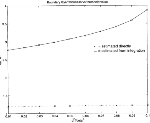
5-3 Number of Nodes with Vorticity Magnitude Less than the Threshold vs. Threshold Value . . . . 55

5-4 Variation in boundary layer thickness with changes in integration end p oint . . . . 59

5-5 Velocity and velocity derivative profiles for various regimes . . . . 60

5-6 Boundary layer surface represented as a function of arc length . . . . 61

5-7 Corner Flow Model . . . . 62

5-8

#

5-9 V) Function contours . . . . 63

5-10 V) and

#

5-11 Areas used in displacement thickness calculation . . . . 64

5-12 Corner flow calculated vs. theoretical displacement curve . . . . 65

6-1 Vorticity plot on the flat plate test case . . . . 68

6-4 6-5 6-6 6-7 6-8 6-9 6-10 6-11 6-12 6-13 6-14 6-15 6-16 6-17 6-18 6-19

Calculated vs. theoretical displacement thickness . . . .

Calculated vs. theoretical momentum thickness . . . . Pipe flow model geometry . . . . Integration Areas for the pipe . . . . Velocity contours on NACA0012 airfoil in Re = 500 flow . . . .

Vorticity contours on NACA0012 airfoil in Re = 500 flow . . . .

Free stream velocity calculation on airfoil in laminar flow, f = 0. Free stream velocity calculation on airfoil in laminar flow, f = 0. Free stream velocity calculation on airfoil in laminar flow, ' = 0. Calculated free stream velocity on laminar flow airfoil model Calculated displacement thickness on laminar flow airfoil model Free stream velocity estimation at ! =0.1 . . . . Free stream velocity estimation at 1 = 0.008 . . . .

Free stream velocity vs. location . . . . Displacement thickness vs. location on upper airfoil surface

Displacement thickness vs. location on lower airfoil surface

1 3 . . . 69 . . . 70 . . . 71 . . . 73 . . . 74 . . . 75 18. 76 27. 77 9 .78 . . . 79 . . . 80 . . . . . 81 . . . . . 82 . . . . . 83 . . . . . 84 . . . . . 85

7-1 Stagnation flow model geometry . . . . 88

7-2 Stagnation flow model with swirl . . . . 90

8-1 Element length vs. the error in displacement thickness . . . . 93

8-2 Element length vs. the error in momentum thickness . . . . 93

8-3 Boundary layer integration volume . . . . 95

8-4 Function integration as convection . . . . 96

8-5 Area integration as a solution to the convection equations . . . . 98

8-6 Typical Triangulated Domain . . . . 100

8-7 Area convection results after 10 iterations . . . . 101

8-8 Area convection results after 30 iterations . . . . 101

8-9 Convected area calculation . . . . 102

8-10 Convection values without damping: Area = 1.01, with damping: Area = 0 .9 7 . . . . 103

8-11 Dissipation constant vs. integrated area value . . . . 104

8-12 Displacement thickness curve . . . . 105

8-13 Displacement thickness curve for coarse grid . . . . 105

8-14 Convecting vorticity on a laminar airfoil model . . . . 106

8-15 Normal curves used for convecting vorticity on the laminar airfoil model107 8-16 70 solution for convection velocity . . . . 108

List of Tables

2.1 Grid study results . . . . 30

4.1 Filtering study results . . . . 46 8.1 Boundary Layer Integration Parameters . . . . 94

Chapter 1

Introduction

This thesis discusses new numerical techniques in the areas of shock detection and boundary layer description. An attempt was made to use the physics of the situation to extract these features, instead of using a more generalized approach, although the goals are sometimes the same. Because the physics of shock waves and boundary layers are so different, they are presented independently.

1.1

Shock Waves

Shocks are a type of compression wave in flow fields that may occur when the veloc-ity of the fluid exceeds the local speed of sound. The state of the fluid as described

by the pressure, velocity and other primitive variables can change radically across

a shock boundary of only a few molecular mean free paths wide. There are many types of discontinuities, but this thesis will only deal with simple shocks; compres-sion discontinuities without heat addition and with constant specific heats. Shock discontinuities are of interest to designers because their strength and location affects drag on aircraft, the functioning of inlets, the efficiency of nozzles and a host of other design problems in fluid mechanics.

image, the purpose of both applications is to find discontinuities in a scalar field that contain large spatial changes in the scalar along with noise and smoothing. In the case of CFD solutions, the noise in the solution is analogous to dispersion and the smoothing is related to dissipation. Figure 1-1 shows the how the pressure across the idealized pressure discontinuity at a shock differs from an actual shock. Dissipation blurs the edges of the shock, making it hard to determine its extent. Dispersion creates the high frequency noise on the edges of the shock.

There are a couple of approaches to detecting shock discontinuities. The first approach is to view it as an edge detection problem and apply the methods that have been developed in that field. Alternatively the physics of shocks can be used to create a detection algorithm that is not applicable to the more general problem. This thesis takes the physics approach since there is not an agreed on 'best' edge detection algorithm and by looking at the physics, it might be possible to formulate a more rigorous detector.

In the past, shock waves have been extracted with an edge detection technique described by Ma, Rosendale, and Vermeer [1]. This technique searches for inflection points in the pressure or density fields by finding areas where the LaPlacian of the

scalar quantity goes to zero. This works because scalar quantities like pressure have their maximum rate of increase at the shock and the second derivative of the scalar goes to zero, as shown in the figure 1-1. However, this detector will pick up other features that are not shocks. There can be expansion waves in a flow solution that are similar to shock features, except pressure and density decrease along streamlines through the expansion. The second derivatives of pressure and density are also zero in quiescent flow like regions far from a body. Both these artifacts have to be removed from the marked areas. One advantage of this approach is that it also captures moving shocks in a transient solution, since pressure and density are invariant quantities; unchanged when the frame of reference is attached to a moving shock.

A second method is to use the pressure gradient to find the value of the mach

number normal to a shock. The approach was outlined by Darmofal [2] and also implemented in Plot3D [3]. Since the shock surface normal will be aligned with the

Ideal shock ---.---Actual shock -Shock region

(D

Location

Figure 1-1: Shock inflection points

pressure gradient vector, the mach number in the direction of this vector is the normal Mach number. A shock is then located where this normal Mach number is greater

than or equal to one.

One disadvantage of this shock finding method is that it will fail to capture some

moving shocks in transient solutions. The mach vector is calculated in the CFD

solution relative to the model frame of reference, but the shock calculation uses the mach vector in the shock frame of reference. For example, a shock traveling in a shock tube can exist when the fluid in the tube is moving at a velocity less than the speed of sound. Only when the Mach number is calculated with respect to the moving shock would this shock be detected. This thesis later describes extensions to the normal Mach number calculation that makes it applicable to moving shocks.

1.2

Boundary Layers

In most flows of engineering interest, the effects of the fluid inertia dominate over the effects of viscosity. The relative importance of the properties is described by the

envision the flow as being composed of two regions; a far field region where viscosity is essentially zero, and a region close to the wall where the viscosity enforces the no-slip condition. The size and shape of the viscous region provides information about drag and flow blockage.

1.2.1

2D Boundary Layers

In real 2D flows, the velocity varies continuously from some free stream value to zero at the wall, so location of the boundary layer edge is subjective. It is often stated as the location where the velocity reaches 95% - 99% of it's free stream value. More

ob-jective measures of the boundary layer are the displacement thickness and momentum thickness. These two measures compare the actual velocity profile to a flow that has a step discontinuity at some distance away from the wall. The approximate velocity profile looks like one of those in figure 1-2. The displacement thickness is related to the velocity of the flow with the following equation.

61 = (1 - -)dn (1.1)

The displacement thickness is a measure of the flow restriction and mass flow deficit

n n n nC n) A CL CD 0) 0 C)D-u(n) 2A

Figure 1-2: Boundary Layer Definitions

momentum deficit caused by the viscous layer, and is defined in relation 1.2.

62= (1 - )dn (1.2)

o U U

1.2.2

3D Boundary Layers

Three dimensional boundary layers are much more complex because of the possibil-ity that the flow changes direction through the viscous layer. Figure 1-3 shows a possible boundary layer profile for a three dimensional flow. One way of describing such flows is to calculate the displacement thickness in the free stream flow direction and a displacement thickness normal to this direction, the cross-flow component as described in Schlicting[4]. The equations for the displacement thickness parallel to the free stream velocity is shown in equation 1.3, where u,6 is the component of the

velocity vector in the direction of the velocity vector at the edge of the boundary layer, 6. Similarly, the equation for the cross-flow displacement thickness is shown in equation 1.4, where un, is the component of the velocity vector in normal to the

velocity vector at the edge of the boundary layer.

6_{iparalle =-}

(1

6_{icross-flow = (1 - )dz (1.4)}

Alternatively, for some geometries, it makes sense to calculate the displacement thickness along perpendicular coordinates that are mapped to a surface. In this case, the definitions for the parallel and cross-flow displacement thickness change to equations 1.5 and 1.6, where x and y are some arbitrary orthogonal vectors, and it is assumed that x is the primary flow direction.

6₁x =j(1 - uj )dz (1.5)

Y N /S Y Z U - _X Y x Y

Side View Top View

Figure 1-3: Three dimensional boundary layer profiles

For example, figure 1-4 shows a curvilinear coordinate system on the wing that is not aligned with the free stream, but is often used in design.

For very convoluted flows, with the cross-flow component switching from positive to negative sign, the integrated cross flow displacement thickness will not show this effect because some of the negative area cancels the positive area of the integral. The integral may be computed with the absolute value of the crossflow velocity component and compared to the normal calculation of the displacement thickness to determine if this is happening. An alternative way to measure these three dimensional boundary layers is to compute the displacement thickness in the local streamwise direction (equation 1.7) and a twist angle from the wall to the free stream (equation 1.8). This in effect unwraps the boundary layer and makes it two dimensional in the rotated coordinate system.

is=

(

Figure 1-4: Swept wing boundary layer integration coordinates

_o fds

0 = )dz (1.8)

o d z

This turning angle calculation suffers from the same problem as the cross flow integral in equation 1.4 because the angle may change sign from the edge of the boundary layer to the wall. Instead, it may be useful to perform the integral on the absolute value of the change in velocity direction and compare this to the total turning angle.

1.2.3

Flow Blockage

One of the advantages of using the displacement and momentum thickness is that these quantities have some physical meaning in two dimensional flows. However, the definitions loose their meaning for more complex geometries, requiring a redefinition for these new cases. In two dimensional flows, the displacement thickness represents the difference in mass flow rate between the actual viscous flow and a flow without viscosity. However, this assumes the body has an infinite extent out of the plane of

flow, without any curvature in this direction. If the wall has curvature normal to the

plane of flow, the integral no longer approximates the mass flow deficit. Figure

volume. As shown in equation 1.9 the definition for 61 can be derived from equating the mass flow rate through an incremental width dz with that obtained by assuming a uniform flow of U0 outside of 61 and 0 less than 61.

(1.9)

p= u(y)dy = Uody

dzp = f1

Y

Front View Side View

Figure 1-5: Boundary Layer on Curved Surface

8 61 dz U00 0 / 5 61 U0 0 ' RI

Without Curvature With Curvature

Figure 1-6: 2D vs Curved Approximations

This can be modified for the case of a cylindrical control volume element with a local radius of curvature, R, as shown in equation 1.10

h =R+6 dp= f R+6 u(r)rdr =

I

This yields equation 1.11 for the displacement thickness as a function of the velocity profile and the local radius of curvature.

/R+6

61 = (+ R2 + f(2 - -)rdr) - R (.1

R Uoo

To check that this equation yields the same result as the two dimensional displace-ment thickness calculation for large radii of curvature, a simple test velocity profile was created and both displacement thickness equations were applied. The velocity profile tested was a linear profile varying from zero at the wall to 1 at the edge of the boundary layer. The thickness calculated for a flat wall is 0.5, while that for the curved wall is shown in figure 1-7. For large radii of curvature, the corrected displacement thickness approaches the two dimensional result, with increasing error in areas of large curvature.

Displacement Thickness vs Radius of Curvature

0.528 0.526 0.524 S0.522 (D 0.52 0.518 (D 0.516 -C S 0.514 - 0-0.512 * 0.51 0.508 0.506 0.504 2 4 OCU6 8 10 Radius of Curvature

circumstances where the surface of the body does not have any local radii of curvature comparable to the boundary layer thickness.

Chapter 2

Stationary Shock Wave Detection

The stationary shock algorithm was developed with a knowledge of the shock geom-etry shown in figure 2-1.

0

0!

SM2

M1

Mn

=

16

D

Figure 2-1: Shock detection test quantity

For any shock, the Mach number normal to the shock has a value of at least one

just

calculate a shock test value at each node. The locations where the test value equals one forms a boundary surrounding the shock location.

This test excludes areas of expansion, since the pressure gradient and the mach vector will have opposite senses, and their dot product will be less than zero.

For three-dimensional models, an iso-surface of M, = 1 was used to visualize the results. The shock feature is surrounded by the M, = 1 iso-surface, and has

a thickness associated with it. In the two-dimensional case, contours of the normal Mach number were created, and the M, = 1 curve forms a boundary for a shock region.

2.1

Shock strength

The relative strength of the shock is of interest to designers, as well as its location. Ideally, the shock strength can be represented by the ratio of some invariant flow variable across the shock. - is measure of the shock strength often used to compute the ratio of the other flow variables across the shock. Unfortunately, the calculated shock region does not correspond to the actual extent of the shock. The shock finding

algorithm relies on high gradients to mark the boundary of the shock region.

However, near the boundaries of the shock, the pressure and density gradients get smoothed due to viscosity in the real shocks and dissipation in numerical shocks. The result is that the detected shock region will not encompass then entire shock as illustrated in figure 2-2. This means that the pressure ratio across the boundary of the detected shock region will be smaller than the actual pressure ratio across the shock.

A different, more direct approach was used to find the pressure values. The

algorithm starts from a node in the shock region and marches in space along the pressure gradient vector. When the pressure is no longer increasing, or is increasing at a very slow rate, then the marching is stopped and the pressure at this point is called P2. A similar procedure is used to find the upstream pressure, but the

Shock location region P2 P2 found P2 P2 found P1 P1 found P1 found P1

Location

Figure 2-2: Computed vs. actual pressure ratio

computationally expensive, but is more analogous to the way an analyst would find the pressure ratio across the shock; by looking at the graph of the pressure normal to the shock. Fortunately, the number of nodes in the shock region is also relatively small and only covers a width of about three cells for the types of solutions tested, so a calculation of this type is not prohibitively expensive; on the order of the computation needed to calculate the shock test quantity.

The shock strength can be represented by the pressure ratio across the shock, which can be calculated by marching in space along the pressure gradient.

2.2

Shock Classification

Their geometry and relationship to physical objects can classify shock waves. This classification can be made automatically once the shock is located.

One classification that can be easily made is for normal or oblique shocks. All that is needed is the angle of the shock with respect to the local velocity. Since the pressure gradient is normal to shock, a test value can be constructed that is the angle

between the velocity vector and the shock surface with the equation 2.1.

arccos (VP - -/q) (2.1)

The only difficulty with this test quantity is that it will change across an oblique shock because the velocity vector direction changes across the shock.

Another classification that can be made is whether the shock is attached (or not) to an object. In this case, it is necessary to see which geometric objects intersect the shock region. If the shock is not attached to a solid surface, then it is a detached shock. This paper does not cover any algorithms to coalesce the shock areas into distinct regions, but clearly this is possible by employing a flood algorithm. Then each shock could have a geometric description, a strength value, an angle, and (if it is a transient model), an associated speed. Unfortunately, it is not always clear how to display the angle and strength values in a meaningful way. For the three-dimensional cases, the angle and strength values were painted on the shock iso-surface, which produced some easily understood results. However, in the two-dimensional case, presenting contours of the strength and angle does not convey the information appropriately. These are single scalar values at a few isolated nodes, and having contours between them and the surrounding areas that do not have values does not make sense. A better method might be to put the numerical values on the shock contour itself.

With a few simple operations, the shocks can be easily classified once located.

2.3

Grid Study

The supersonic ramp test case had the geometry of figure 2-3. The shaded area is the region of the model that was used to plot the results and grids. Three different uniform grids were generated for the same geometry to determine the sensitivity of the detector to grid size. Figure 2-4 shows the three grids that were used for the experiment.

open

Figure 2-3: Ramp model

SEEM

---Coarse Grid

Fine Grid

Highly Refined Grid

M = 3

0

Pu

shock. The larger the element size, the larger the indicated shock. Figures 2-5, 2-6 and 2-7 are contour plots of the normal Mach number, starting at M, = 1 in the region of the wedge.

Figure 2-5: Shock contours on the coarse grid

Figure 2-6: Shock contours on the more refined grid

The results in table 2.1 show that the shock algorithm displays shock thickness as a linear function of element size. The shape of the shock region not only locates the shock, but also can point to a lack of mesh refinement in the area.

The numerical model used to solve the problem also greatly effects the shape of the shocks. Some CFD solution algorithms are better suited to capturing the sharp

Figure 2-7: Shock contours on highly refined grid

Number of Shock thickness (num elements cells)

5272 3

13801 3

20942 3

discontinuities. The larger the effective dissipation, the more spread out the shock and the more cells involved.

2.4

Supersonic projectile

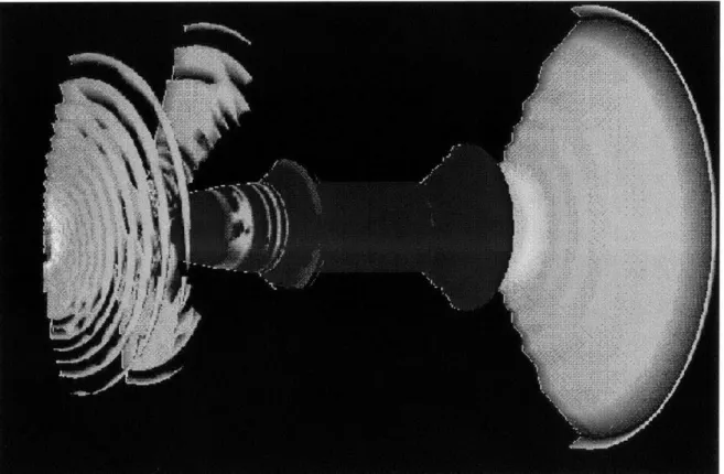
The same shock finding algorithms were applied to the results of a much larger three-dimensional viscous solution; a projectile in a Mach 1.2 flow. The image in figure 2-8 shows the shock iso-surface painted with the calculated pressure ratio. The grid is only refined near the body, so the shock appears jagged at any distance from the body. The highest pressure ratio occurs at the center of the oblique shock just in front of the nose, and has a value of 1.5.

Figure 2-8: Three dimensional shock representation on a projectile model in mach 1.2 flow

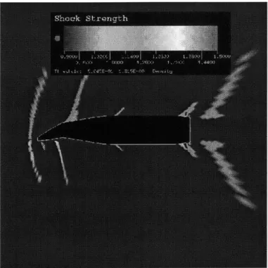
Figure 2-9 shows a two dimensional slice of the same model. A couple of features appeared that were somewhat puzzling. Note that there was an indicated shock after the first bend on the top of the shell, which should really be followed by an expansion.

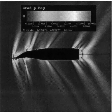
Closer examination of the pressure gradient magnitude shown in figure 2-10 shows that there is an expansion immediately following the turning, then a sudden increase in pressure that the shock finder has picked up. This filter is not picking up the expansion waves.

Figure 2-9: Shock strength false color image

The shock algorithm picked out the bow shock and compressive bend at the bot-tom front of the shell, but also detected some other interesting features. In fact, the designers of the projectile are still arguing over the cause of these compressions after the initial expansions.

Chapter 3

Transient Shock Wave Detection

The assumptions made in constructing the previously described shock finding tech-nique no longer apply when the shock is moving. To locate a shock with the previous method, it is necessary to assume that the observer is traveling with the shock and all velocities are measured with respect to this translating frame of reference. However, since all velocities are calculated in the model frame, there has to be a correction applied to the test equation to account for the moving shock. The equation 3.1 shows what this term must be, basically a time derivative of the pressure.

1 1 Dp 1 1 dp M - VP

- - - + (3.1)

|V PIa Dt |V PIa dt + V P|

It is more computationally expensive to approximate time derivatives directly, since that would require the storage of multiple time steps. So, the time derivative of pressure was calculated based on relations that equate it to a spatial variation of the state variables. Equation 3.2 applies to isentropic flows.

dp = a2d p (3.2)

an equation for an invariant test quantity that can be used to locate moving shocks.

(3.3) =p _{- -a2 V -(pq)}

dt

From equations 3.2 and 3.3, equation 3.1 becomes: 1 1 Dp I V PI a Dt 1 = 7 a P -(pq) I|V P I +

IVP

A shock is then located when this quantity equals or exceeds one.

In the general case, pressure can be related to the internal energy and velocity of the flow with equation 3.5.

1

p = (-y - 1)[pE - -(pq - (pq] p

(3.5)

Taking the time derivative of this quantity will yield the required correction term, equation 3.6.

dp _d(pE)

-dt dt

1 2dp

+-q _{2 dt}|] (3.6)

Substituting equation 3.3 into equation 3.6, and replacing the time derivatives with their equivalents from the mass and momentum equations yields equation 3.7.

dp - (7- 1)[- 7 -(pqH) +

dt

1 q2

q - (,7P + Vpfig 2 2q V -(pq'] (3.7)

This is the generalized correction term needed for transient problems.

3.0.1

Translating normal shock in a tube

A model of a moving normal shock in a channel was created to investigate the behavior

of the shock finding algorithm and the effect of the transient modification. Two (3.4)

0d

q .-- (pq

separate runs were done, the first had the initial conditions shown in the figure 3-1. P2/P1 = 5

Shock

Figure 3-1: Transient Shock Model

Shock relations were used to set up the initial conditions for the model. The formulas for moving normal shock waves with constant C, and C, were applicable in this case. However, these formula assume that the upstream speed, U1 is 0, so a

correction had to be made to produce the correct initial conditions for the flow. For the first run, the pressure ratio was chosen to be less than the pressure ratio required for a standing shock in M=3 flow (10.33). This required that the shock move toward the right in the positive X direction. The speed of the shock traveling into a stationary fluid, W, was calculated with the equation 3.8. Since the upstream velocity was not

zero, the actual speed of the shock had to be corrected with equation 3.9.

7+ 1 P2

W = ai ( P 1) + 1 (38)

W, = U1 - W (3.9)

The shock test scalar was calculated with the isentropic transient correction equa-tion (equaequa-tion 3.4), that was simplified for this particular example. The Y component

the following.

1

ID

| V PI a Dt |~v P| dx |V P|

The derivative of the density times the X velocity was then expanded, yielding the final equation.

1 1Dp 1 du dp 1M-VP)

Iv~a t= -a ~ ( p + -U) + (3.11

| V P| a Dt |1 V P| dx dx | V P|

Results indicated that the pressure variation across the shock has some interesting features that are problematic for the shock finding algorithm. The shock started at X=0, and is moving to the right in the positive X direction. As it moves, the shorter wavelengths that makeup the initial discontinuity move at a slower speed than the longer wavelengths. This difference in speed is a numerical artifact of the time stepping method used in the CFD solver. As time progresses, high frequency pressure oscillations show up behind a moving shock, as shown in the figure 3-2.

0.10 0.08 0.07 i 0.06 C) 0.05 Dispersion effect 0.03 0.02T -2.00 -1.33 -0.67 0.00 0.67 1.33 2.00 X location

Figure 3-2: Pressure Distribution

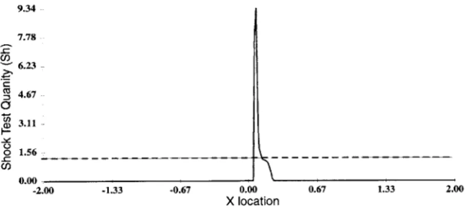
Figure 3-3 is a plot of the shock scalar with the isentropic transient correction.

A filter has been applied to eliminate the pressure gradients caused by dispersion.

The dashed line on this and following figures represents the threshold for a shock. Everything above one is marked as a shock region.

9.34 7.78 C/) S4.67 0 o 1.56--_ U) 0.00 --2.00 0.00 X location

Figure 3-3: Shock Scalar

is clearly moving to the right, as expected.

-1.33 -0.67 1.33 2.00

X location

Figure 3-4: Shock Scalar at 6t

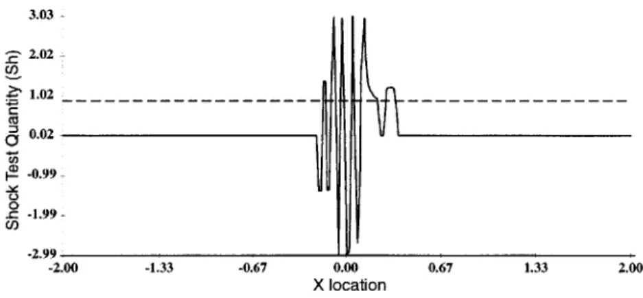
The results of this experiment point to the importance of choosing a threshold value for the magnitude of the pressure gradient. Because of the slower wave speeds of the higher frequency pressure waves, oscillations in the pressure gradient take place behind the shock. These pressure gradient increases are enough to skew the results and show up in the shock detection values as a group of shocks behind the actual position as shown in figure 3-5.

From the above experiment, it was noted that it did not matter if the transient correction was used or not, a shock would still be indicated. This was because the

-1.33 -0.67 0.67 1.33 2.00 -c U) CI) 8.03 6.69 5.35 4.01 2.68 1.34 0.00 --2.00

3.03 2.02 1.02 _ _ _ _ _ _ _ _ _ W 0.02 -0.99 0 0 - -1.99-.2.99 -2.00 -1.33 -0.67 0.00 0.67 1.33 2.00 X location

Figure 3-5: Shock scalar with unfiltered pressure gradient

when the upstream Mach number is less than one. The upstream Mach number was set to 0.9, and the pressure difference was set to 3.0, which will produce a normal

shock moving in the negative X direction of figure 3-1.

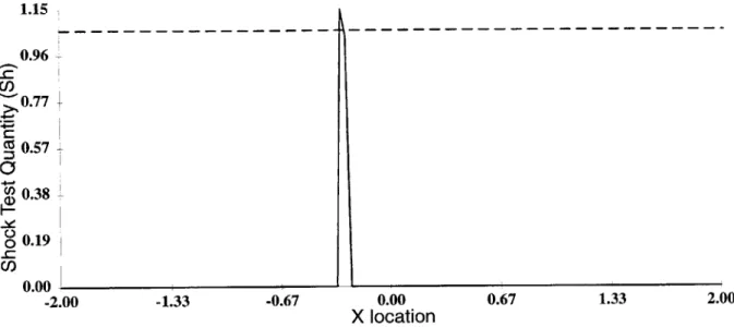
The results of applying these boundary conditions are shown in the following fig-ures. In figure 3-6, the normal Mach number is plotted against the model x coordinate. The normal Mach number never exceeds unity, which by the previous test indicates that no shock is present in the flow. However, the shock test scalar in figure 3-7 does exceed unity at the shock, indicating that the shock is indeed present. The correction term has made it possible to locate the shock.

0.60 -0.50 8 0.40 E Z 0.30 0.20 0.10 0 z -0.00 -2.00 -1.33 -0.67 0.00 0.67 1.33 2.00 X location

Figure 3-6: Normal Mach Number vs. Location

The experimental results were then compared to the theoretical location of the shock at any given time, calculated with the following equation, where x is the

loca-1.15 0.96 Cl) 0.77 C 0.57 0.38 F-o 0.19 U/) 0.00 -2.00 -1.33 -0.67 0.00 0.67 1.33 2.00 X location

Figure 3-7: Shock scalar vs. Location

tion, t is time and W, is calculated with equations 3.8 and 3.9.

X = Wst (3.12)

Figure 3-8 is a plot of the difference between theoretical and measured shock location vs. time.

The experimental shock location was measured two ways, first by the location of the maximum pressure gradient magnitude, and secondly by central location of the shock region.

Since the shock region actually covers about 3 cells in width, or 0.09 units, the theoretical shock location and pressure gradient maximum both occur well within the region at all times.

0.015 0.01 + 0.005- 0--0.005 - -0.01-- 0.0150.02 --0.025 . 0 0.2 0.4 0.6 0.8 1 1.2 time

Figure 3-8: Theoretical vs. Experimental Shock Location - - Maximum Pressure

Gradient -- Shock Value

--Chapter 4

Filtered Shock Detection Results

The previous results show that this shock finding algorithm produces some falsely indicated shock regions. This is partially due to small numerical errors in the gradient away from the shock. As the gradient of pressure goes to zero in the far field, errors in the shock test function build as shown in the following equation, where 6 is a small variation in the quantity.

M(vP +6ovP)

6

yP

| V P + 6 P |67 P|

l

To remove these false indications, three filtering techniques have been applied to the problem. The techniques start with an iso-surface constructed where the value of the shock test scalar is 1.0 and they reject a subset of the triangles that makeup that surface. The first technique enforces the property that the pressure gradient is normal to the shock surface. This technique removes all shock surface triangles that do not pass the test in the following equation, where n is the normal of the surface triangle, and c is a threshold value between 0 and 1.

I

V

pres-discontinuities should only occur in regions of relatively high gradients. The problem is to determine the meaning of a 'relatively' large gradient and set an appropriate threshold. To accomplish this, all the triangles were divided into groups based on the value of the pressure gradient magnitude at their centers. The count of triangles in each group forms a curve. The threshold was chosen where the derivative of this curve goes to zero. This method of setting a threshold assumes that the actual shock surface is located in a region of high gradients and that changing the threshold by some small amount will not change the number of triangles in the surface.

Note that setting a pressure gradient magnitude threshold can be done before the shock iso-surface is constructed by applying the filter to the nodal shock scalar values.

If the node does not pass the pressure gradient magnitude test, the shock value can

be set to 0. Applying a filter to the nodal values has the advantage of producing a more connected shock surface, without disjoint triangles missing.

A third technique removes all the triangles that do not have jumps in density and

temperature that correspond to normal shock relations. For a moving normal shock, equations 4.3 and 4.4 state the relationships between the pressure jump across the shock and density and temperature ratio, respectively.

1 1+ + P2 P2_ Y-1 Pi _(4.3) Pi +1+Pa y-1 Pi T1 p11+lP2 ,Y-1 Pi

The difficulty with this filtering technique is that the extent of the shock needs to be known before hand, so that the pressure, temperature and density ratios can be accurately measured. To overcome this problem, a number of measurements of the pressure temperature and density were made on both sides of the surface triangles, then the two measurements that best fit the shock relations were used to determine if the triangle should be rejected. A fitness function was constructed that, given the measured pressure ratio at two points on either side of the triangle, compares the measured temperature ratio to the temperature ratio computed with equation 4.4

and the measured density ratio with the computed density ratio of equation 4.3 and produces a value of 1.0 in the case where the measurements match theory, and less than 1.0 otherwise.

f(Pi,P2,Ti,T 2,Pi,P2) <= 1.0 (4.5)

If none of the points on either side of the triangle can produce a fitness value of

greater than some threshold, the triangle is removed.

To compare the filtering techniques, a measure of difference between the shock test value fields was constructed. The comparison works from a baseline that is assumed to be the actual shock, then the comparison is run against the results of the unfiltered algorithm and the solution with the various types of filtering. The difference measure is constructed by gathering the centerpoints of all the triangles in the shock surface,

F, then all the points that have a shock value greater than 1 in the baseline and test

solution are removed from F. The total difference value is the sum of the absolute value of the difference between the values of the baseline and test solution at the points in C. The final comparison function takes the total difference and divides it by the final number of triangles in the shock surface.

C=F-BnF (4.6)

Figures 4-1, 4-2, and 4-3 show the results of applying some of the filtering tech-niques, and why they are necessary. In this case, the solution being examined is an

Figure 4-2: Transient shock algorithm without filtering

Figure 4-3: Transient shock algorithm with pressure gradient magnitude filter

inviscid converged flow on a 300,000 element f18 aircraft model traveling in subsonic flow. Because the solution has run to convergence, the stationary and transient shock finding algorithms should produce the same results, which as figure 4-2 shows, is not the case. The transient algorithm generates noise and false indications. However, these false signals can be removed with filtering to produce a shock surface that is very similar to the stationary shock finding results. Figure 4-3 shows the results of

running the transient shock finder through a pressure gradient magnitude filter. Table 4.1 is a collection of the results from passing the transient shock finder through various combinations of the three filtering algorithms. The results in table 4.1 indicate that the pressure gradient magnitude filter alone is better than when used in combination with the other two. This became more evident in looking at the graphical output, where there would be a fairly continuous shock surface at the end of the pressure gradient magnitude filter, with some additional outliers. Applying the normal filter or jump condition filter to these results did not get rid of the outliers, but only removed some of the surface triangles enclosing the shock region, making the

test case Comparison function value no filtering 0.57 I V PI filter 0.105 I V PI and nor- 0.223 mal filter I V P1 and jump 0.104 filter jump filter 0.567

Table 4.1: Filtering study results

final result worse than the result from the pressure gradient magnitude filter alone.

4.1

Transonic Aircraft

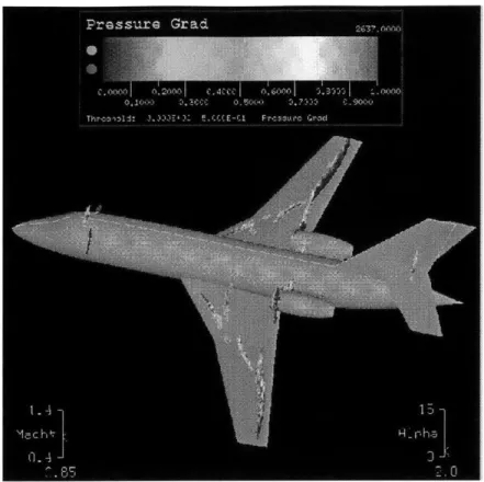
The transient modifications were tested on a relatively large model (1 million el-ements) of an aircraft traveling in transonic conditions (mach 0.85) to see if the unsteady shock finding algorithm could produce useful results on a realistic model. Figure 4-4 shows the results of applying the steady state shock finding algorithm to the converged solution. An iso-surface has been constructed where the normal Mach number equals one, and this iso-surface is painted with the pressure gradient magni-tude as an indication of the shock strength. Note that the thickness of these shock regions is quite small due to the highly refined mesh. Figure 4-5 is of the same model, but the iso-surface is now plotted on the results from the unsteady shock algorithm.

Since the solution has converged, the unsteady and steady shock results should be identical. While this was true of the larger shock features, the unsteady algorithm also produced some false indications. It was necessary to threshold out these regions with the pressure gradient magnitude. Even when this was done, some false indications remained, especially at the leading and trailing edges of the wing. This result was in agreement with the one-dimensional results, where it was also necessary to filter out

Figure 4-4: Shock detection algorithm applied to a Euler solution of an aircraft model

The shock finder captured some fairly complex shock structures that would be difficult to find almost any other way.

Figure 4-5: Unsteady shock detection algorithm applied to a euler solution of an aircraft model

Chapter 5

Boundary Layer Detection

This chapter presents the basic algorithm that was developed for determining the boundary layer thickness, as well as a more formal discussion of the different boundary layer measures and their characteristics. Later chapters are devoted to applying the algorithm to various velocity profiles from exact solutions of the boundary layer equations. In these test cases, the theories were applied analytically to see if they would be valid for the velocity profile of the solution. Then any difference between the analytic and numerically obtained results was investigated. Even if the boundary layer thickness was determined exactly using analytic means, it is important to know how discretization introduces error into the calculation. Ideally a CFD solution has 10-20 points in the boundary layer, so if a numerical method cannot resolve the boundary layer thickness with information from these few points it is essentially useless, even though it may give exact answers for an analytic, smooth velocity profile.

5.1

Boundary Layer Definition

The algorithms developed here try to determine a characteristic boundary layer thick-ness, but what is that exactly? In general, the boundary layer is the region in the neighborhood of a solid body where high velocity gradients and boundary conditions on the body make viscosity influence the flow, while outside of this region viscosity may be neglected. It can be shown that the characteristic thickness of this region is

related to the square root of the Reynolds number, and for flows of engineering inter-est, this makes the boundary layer thickness very small; on the order of a percent of the characteristic length of the flow. With this in mind, it is possible to get an idea of the geometry of the boundary layer on a solid body. The picture becomes that shown in figure 5-1, where the curvature of the wall becomes large relative to the bound-ary layer thickness, and the local normal varies slightly in the streamwise direction. Neglecting three-dimensional effects, the velocity magnitude goes from zero up to a "free stream" value where it is no longer affected by viscosity. This "free stream" velocity is not necessarily the velocity far from the body, but the velocity just outside the region where viscosity has an influence. So, if one knows the free stream velocity, the boundary layer thickness can be defined as the location along the normal where the velocity is some percentage of the free stream velocity like -L _U = 0.99 or I _U = 0.95.

Unfortunately, the way to define free stream velocity is to find the velocity outside of the boundary layer, making a circular argument for finding the boundary layer thick-ness. What if the flow equations could be solved on the same geometry, but with a

U0

Figure 5-1: Typical boundary layer profile

zero viscosity? Would the velocity at any point on the surface in the inviscid solution be the free stream velocity? Well, the short answer is no, not for all cases. Imagine

Typical fully developed viscous channel solution

u(x) _{u(x) = U(X)1}

0

Displacement thickness approximation Mass flow = const

Umax Umax

Inviscid approximation

u(x) = Uave

flow are shown in the equation 5.2. 0 0 1 ld LUy (51) 0 jL (U2 _ U2)d (P1 - P2)L - Fwaii (5.2)

Since this is a fully developed flow, u is not a function of x, therefore the pressure difference from station 1 to 2 balances the shear force exerted by the wall. Compare this solution to a problem with the same boundary conditions, but without viscosity and shear stress. Without the shear stress term and given a finite pressure difference, the flow will accelerate through the channel. So, picking a single free stream velocity from the inviscid solution is not possible. As an alternative, an inviscid solution could be generated where the pressure difference was set to zero, and the mass flow rate was the same as in the viscous solution. The viscous velocity profile cannot be uniform, since the velocity has to go to zero on the boundaries. Therefore it goes from zero at the wall to some maximum, and then back to zero at the other wall, with the area under the curve representing the mass flow rate. However, the inviscid solution will be a uniform velocity across the channel with the velocity times the height of the channel equal to the viscous mass flow rate. Because of the difference

in the shape of the velocity profiles, the inviscid flow velocity will be less than the

maximum viscous velocity. If the definition of the boundary layer is the region where

the flow is influenced by viscous forces, then the fully developed channel flow only has one point outside of the boundary layer, the center of the channel and location of maximum velocity. With this definition, the maximum velocity in the viscous solution would be the "free stream" velocity. But this conflicts with the definition of free stream velocity that is the velocity at the surface in an inviscid solution on the same geometry, because that velocity is a mean velocity across the channel and less than the maximum. Having an inviscid solution on the same geometry and with the same boundary conditions did not make the problem of finding the boundary layer

5.2

Possible Detection Methods

For completeness, a few ways of finding the extent of the boundary layer are presented, along with some reasons for and against their usefulness. The following are the criteria that were used for comparing boundary layer detection algorithm

1. Uses only the vector of unknowns from the CFD simulation or quantities derived

from these. This includes the mass, momentum and energy at each point. 2. Works irrespective of wall geometry

3. Does not need to know the velocity on the edge of the boundary layer before

hand

4. Works for wakes and separated regions

5. Works for laminar and turbulent boundary layers

5.2.1

Potential flow quantities

One technique is to use the idea that some scalar flow quantities do not change in potential flow regions. Boundary layers can be located by marking the regions where

these variables are changing, or differ from the free stream values. For this technique to work, a threshold has to be calculated or set that is a physically meaningful bound-ary layer edge. There has to be a value of a field variable, where if below or above this threshold, the location is no longer in the boundary layer.

Entropy is one such field variable that is a constant in the potential flow region, and generated in the boundary layer. Unfortunately it may also generated in shock waves and in areas of heat addition, so these areas would have to be somehow removed from the boundary layer detector. An entropy detector also suffers from the problem of choosing a threshold value, because entropy is not guaranteed to be the same across all the streamlines before entering the boundary layer. There are situations in isentropic flows, where the entropy does not change along a streamline, but does change from streamline to streamline. Another difficulty is that the value of the