Bayesian tuning and bandits : an extensible, open source library for AutoML

Bayesian Tuning and Bandits: An Extensible, Open

Source Library for AutoML

by

Laura Gustafson

Submitted to the Department of Electrical Engineering and Computer

Science

in partial fulfillment of the requirements for the degree of

Masters of Engineering in Electrical Engineering and Computer Science

at the

MASSACHUSETTS INSTITUTE OF TECHNOLOGY

June 2018

© Massachusetts Institute of Technology 2018. All rights reserved.

Author . . . .

Department of Electrical Engineering and Computer Science

May 25, 2018

Certified by. . . .

Kalyan Veeramachaneni

Principal Research Scientist

Thesis Supervisor

Accepted by . . . .

Katrina LaCurts

Chairman, Masters of Engineering Thesis Committee

Bayesian Tuning and Bandits: An Extensible, Open Source

Library for AutoML

by

Laura Gustafson

Submitted to the Department of Electrical Engineering and Computer Science on May 25, 2018, in partial fulfillment of the

requirements for the degree of

Masters of Engineering in Electrical Engineering and Computer Science

Abstract

The goal of this thesis is to build an extensible and open source library that handles the problems of tuning the hyperparameters of a machine learning pipeline, selecting between multiple pipelines, and recommending a pipeline. We devise a library that users can integrate into their existing datascience workflows and experts can contribute to by writing methods to solve these search problems. Extending upon the existing library, our goals are twofold: one that the library naturally fits within a user’s existing workflow, so that integration does not require a lot of overhead, and two that the three search problems are broken down into small and modular pieces to allow contributors to have maximal flexibility.

We establish the abstractions for each of the solutions to these search problems, showcasing how both a user would use the library and a contributor could override the API. We discuss the creation of a recommender system, that proposes machine learning pipelines for a new dataset, trained on an existing matrix of known scores of pipelines on datasets. We show how using such a system can lead to performance gains.

We discuss how we can evaluate the quality of different solutions to these types of search problems, and how we can measurably compare them to each other.

Thesis Supervisor: Kalyan Veeramachaneni Title: Principal Research Scientist

Acknowledgments

I would like to thank Kalyan for his guidance through out the project. His willingness to talk through ideas, make suggestions, and assist when needed were crucial to the success of the project.

Additionally, I would like to thank my parents, MaryEllen and Paul, for their constant support throughout my life. Without their continued love and encouragement, I never would have gotten to where I am today. I would also like to thank my older brother, Kevin, for his support.

Finally, I would like to thank Kali, Anne, and Brittany for their support over the past year. While I may now have another BTB, I would like to thank the members of Burton Third for having been there through thick and thin and ensuring I never was lonely.

Contributions

We would like to acknowledge the contributions of Carles Sala and Micah Smith in the design of the API, the open-source release, and general development of the BTB library.

We acknowledge generous funding support from Xylem and National science foundation for this project.

Contents

2 Tuners and Selectors 29 2.1 Tuner . . . 29 2.1.1 API Changes . . . 29 2.1.2 User API . . . 30 2.1.3 Contributor API . . . 31 2.2 Selector . . . 35 2.2.1 User API . . . 35 2.2.2 Contributor API . . . 36 3 Recommender 39 3.1 Overview of recommender problem . . . 39

3.1.1 Related Work . . . 40

3.1.2 Notation . . . 40

3.2 Methods . . . 41

3.4 User API . . . 45

3.5 Contributor API . . . 46

3.6 Evaluation . . . 49

3.6.1 Data . . . 49

3.6.2 Storing the results . . . 51

3.6.3 Evaluation of Results . . . 52

3.7 Results . . . 54

3.7.1 Performance Graphs . . . 56

3.7.2 Improvement Upon the Results . . . 57

4 _{Current usage of BTB} 59 4.1 DeepMining . . . 60

4.2 MIT TA2 System . . . 62

4.3 ATM . . . 65

5 Open Source Preparation 67 5.1 Increased Functionality . . . 67

5.1.1 Handling Categorical hyperparameters . . . 67

5.1.2 Abstraction of Logic for Hyperparameter Transformation . . . 69

5.2 Testing . . . 70

5.3 Examples . . . 71

6 Getting contributions from experts 73 6.1 Evaluating methodological contributions . . . 76

6.1.1 Setting benchmarks . . . 77

6.1.2 Evaluation Metrics . . . 79

6.1.3 Results of an experiment . . . 81

6.2 Automation . . . 83

6.3 Workflow for creating and merging a new method . . . 85

7 Conclusion 87 7.1 Key Findings and Results . . . 87

7.2 Contributions . . . 87

List of Figures

1-1 Diagram showcasing how a tuner works. Hyperparameter sets tried previously and their scores are passed to the tuner, which proposes a new set of hyperparameters. A new pipeline is run with the hyperparameters, the resulting score is added to the data, and the tuning continues. . . 21 1-2 Gaussian kernel density estimator of performance on hutsof99_logis_1

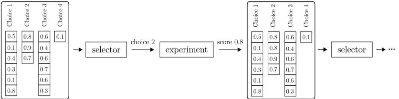
for three different classification techniques: logistic regression, multi-layer perceptron and random forest. The performance for each of the classifiers is aggregated over tuning a variety of different hyperparameter search spaces. . . 22 1-3 Diagram showing how a typical selector system works. Data pertaining

to past scores for each of the choices is passed to the selector which outputs a choice to make. The score that results from that choice is added to the data, and the process continues. . . 23 1-4 Diagram showing data used in a recommender system. We know the

performances of some solutions on existing problems, along with the performance of a few solutions on a new problem. We can use the known problem data to make recommendations for the new problem. 25 1-5 Diagram showing how data flows to and from a recommender system.

At each iteration, the matrix is passed to the recommender. The recommender’s proposal is tried on the new row in an experiment, and the matrix is updated. . . 25

2-1 A Python code snippet illustrating how to use a tuner’s user API. The code illustrates how to use a tuner to tune a number of estimators hyperparameter between 10 and 500 and maximum depth of a tree between 3 and 20 for a random forest. The code snippet is given training data 𝑋, 𝑦 and testing data 𝑋𝑡𝑒𝑠𝑡 and 𝑌𝑡𝑒𝑠𝑡. The tuner does not

require the user to store any scoring data on their end. The user only has to call two methods after initialization, add to add new data to the tuner and propose to receive a new recommendation from the tuner. 32 2-2 Interaction between the user API and developer-overridden methods

for the tuner class add method. . . 33 2-3 Interaction between the user API and developer-overridden methods

for the tuner class propose method . . . 33 2-4 Relationship between six different tuners. Includes the developer API

functions overridden to implement the tuner. . . 35 2-5 Python code snippet illustrating how to use a selector alongside a tuner

to choose whether to next tune a random forest or an support vector machine (SVM) classifier. The n_estimators is a hyperparameter for a random forest and has the range [10, 500]. The c is a hyperparameter for SVM and has the range [0.01, 10.0]. The code snippet is supplied with training data 𝑋, 𝑦 and testing data 𝑋𝑡𝑒𝑠𝑡 and 𝑌𝑡𝑒𝑠𝑡. TUNER_NUM_ITER

specifies the number of iterations of tuner when a particular pipeline (in this case only a classifier) and SELECTOR_NUM_ITER specifies the

number of iterations for the selector. . . 36 2-6 Interaction between user-facing API and developer overridden methods

for selector class select method . . . 38

3-1 Python pseudo-code snippet illustrating how to use a recommender’s user API . . . 46 3-2 Interaction between user API and developer-overridden methods for

3-3 Interaction between user API and developer-overridden methods for recommender class propose method . . . 48 3-4 pbest at different iterations for matrix factorization and uniform

rec-ommenders on visualizing_ethanol_1 dataset . . . 56 4-1 An illustration of how data flows through a system that uses a tuner,

such as DeepMining or TA2, which shows how score and hyperparameter information is shared within the system. . . 59 4-2 Python pseudo-code snippet illustrating how DeepMining uses BTB to

score hyperparameter combinations in parallel. . . 61 4-3 Python pseudo-code snippet illustrating how MIT TA2 uses BTB to

yield the best possible pipeline over a series of iterations. . . 63 4-4 LSTM Pipeline Data Flow Diagram . . . 64 4-5 Diagram showing how information including scores, hyperparamters,

and choices flows through ATM. . . 65 6-1 Histogram of a search problem with a difficult distribution. While it

is easy to perform well on this search space, it is hard to model the distribution to consistently outperform a uniform tuner. This search problem is searching the KNN hyperparameters described in Table 6.2 on housing_1 dataset. . . 83 6-2 Comparison of the best ranking hyperparameter combination given a

MLP pipeline on chscase_health_1 dataset. The grid for this search problem had 1000 different hyperparameter sets. . . 84 6-3 Comparison of the best mean f1 score yielded by a pipeline tuned for a

List of Tables

3.1 Potential scores for three datasets A, B, C on 5 pipelines 1,2,3,4,5 . . 43 3.2 Score rankings corresponding to table 3.1 . . . 44 3.3 List of datasets used in evaluation of matrix factorization-based

recom-mender. . . 50 3.4 Storage of Results of recommender Evaluation . . . 52 3.5 Maximum p_best, Number of Wins and C.I. Lower Bound Results

from Recommender Evaluation on 30 Datasets; Each Experiment Ran 20 Times . . . 54 3.6 Performance Increase Percentage Results from Recommender

Evalua-tion on 30 Datasets; Each Experiment Ran 20 Times . . . 54 3.7 Statistical Analysis of Results from Recommender Evaluation on 30

Datasets; Each Experiment Ran 20 Times . . . 55 4.1 Table of the LSTM Text pipeline’s tunable hyperparameters, ranges,

and description. . . 65 5.1 Example showing how the values of a categorical hyperparameter can

be mapped to a numerical representation and back . . . 68 6.1 List of datasets used in tuner evaluation . . . 77 6.2 The model type and tunable hyperparameters for the search problems

used in tuner evaluation . . . 78 A.1 User API for selectors . . . 90 A.2 Developer API for selectors . . . 90

A.3 User API for tuners . . . 91

A.4 Developer API for tuners . . . 92

A.5 User API for recommenders . . . 93

A.6 Developer API for recommenders . . . 93

A.7 API of Hyperparameter BTB Class . . . 94

A.8 Results from tuner evaluation on 20 20 search spaces; Each experiment was run 20 times . . . 95

A.9 Statistical analysis of results from tuner evaluation on 20 search spaces; Each experiment was run 20 times . . . 95

Chapter 1

Introduction

In recent years, the success of machine learning (ML) has lead to an increased demand for ML techniques in fields such as computer vision and natural language processing. This in turn has led to a demand for systems that can help automate aspects of the process that involve humans, such as choosing a machine learning model or selecting its hyperparameters. These systems have become a part of the rapidly growing field of automated machine learning (AutoML) [17], which seeks to reduce the need for human interaction to create and train machine learning models.

In this thesis, we create a general purpose open source library, Bayesian Tuning and Bandits (BTB), that enables the following search problems within AutoML: tuning the hyperparameters of a machine learning pipeline, selecting between multiple pipelines, and recommending a pipeline.

We envision the people who will interact with BTB will fall into two categories: users and expert contributors. Users are the people who will integrate BTB into their existing data science workflows, but will not need in-depth knowledge of the field of AutoML in order to use the library. Expert contributors are AutoML or ML experts who will contribute to the BTB library by writing their own novel methods for solving the tuning, recommendation, or selection problems.

Our goals for the library are twofold: First, that the library fits within a user’s existing workflow naturally enough that integration does not require a lot of overhead, and second, that the three search problems are broken down into small and modular

pieces to give expert contributors maximal flexibility. As there is debate about different methods, we have taken steps to ensure that the library is flexible enough to easily swap out different methods. While the field of AutoML is growing rapidly, no existing libraries cleanly and concisely deliver their capabilities to users while simultaneously bridging the gap between experts in AutoML and data scientists solving real world problems using AutoML.

1.1

Overview of Problems

The problems we choose to address in the BTB library are:

1. Tuning the hyperparameters of a pipeline to maximize a score.

2. Selecting among a series of options in order to maximize the score of the option.

3. Leveraging the performance of different pipelines on previous datasets to recom-mend a pipeline for a new dataset.

1.2

Tuning

Tuning tackles the simplest of all search problems. It involves a fixed pipeline where only the hyperparameters are tuned to maximize the score. For example, take tuning a random forest machine learning model. We could choose to search for the two hyperparameters: max_depth, the maximum depth allowed for any tree in the forest, and n_estimators, the number of trees in the forest. We can set the ranges for search at [4, 8], and [7, 20] respectively. For a pipeline 𝑃 that has 𝑘 hyperparameters, 𝛼1...𝛼𝑘,

and a function 𝑓 that scores 𝑃 with the specified hyperparameters, we formally define the tuning problem as:

𝐺𝑖𝑣𝑒𝑛 : 𝑃 (𝛼1...𝛼𝑘), 𝑓 (·)

𝐹 𝑖𝑛𝑑 : 𝑎𝑟𝑔𝑚𝑎𝑥𝛼1...𝛼𝑘⟨𝑓 (𝑃 (𝛼1...𝛼𝑘)⟩

result 0.7 proposal

_...

Figure 1-1: Diagram showcasing how a tuner works. Hyperparameter sets tried previously and their scores are passed to the tuner, which proposes a new set of hyperparameters. A new pipeline is run with the hyperparameters, the resulting score is added to the data, and the tuning continues.

The scoring function typically calculates a desired metric via cross-validation. This task can usually be accomplished by what is known as a black box optimization. In this approach, :

– A meta-model is formed that identifies the functional (or probabilistic) relation-ship between the hyperparameters and the pipeline scores.

– Scores are predicted for a series of candidate hyperparameter sets using the meta-model.

– A specific hyperparameter set is chosen based on these predictions.

The AutoML community has developed a number of methods for meta-modeling, including a Gaussian process-based regression and a tree-structured parzen estimator [3]. This type of search also has many other applications, including tuning the hyperparameters of a compiler to maximize speed [24].

Figure 1-1 shows a typical integration with a tuner. The user has a pipeline that they want to tune, which requires a series of hyperparameter values to be specified in order to run. At each time step, the user has a matrix of hyperparameter sets that were tested before, along with their associated scores. The user passes this to the tuner, which creates a meta-model and then proposes a new hyperparameter set to try. The user sets these hyperparameters for the pipeline, fits the pipeline and records the resulting score. The newly tried hyperparameters set and score are added to the

Score Increase −→

Probabilit

y

Distribution

Multilayer Perceptron Random Forrest Logistic Regression

Figure 1-2: Gaussian kernel density estimator of performance on hutsof99_logis_1 for three different classification techniques: logistic regression, multilayer perceptron and random forest. The performance for each of the classifiers is aggregated over tuning a variety of different hyperparameter search spaces.

matrix for the next iteration. The tuning process continues until a fixed number of iterations are finished or a desired score is achieved.

1.3

Selection

Selection is the next level of search. Here, we have multiple possible pipelines, each with their own hyperparameters that can be tuned. This search problem is complex because we do not know 𝑎𝑝𝑟𝑖𝑜𝑟𝑖 which pipeline will yield the best score when fully tuned. This problem essentially involves allocating resources for tuning different machine learning pipelines.

Formally, for a set of 𝑚 pipelines (or choices) 𝑃𝑖 that each has 𝑘𝑖 hyperparameters,

we define the selection problem as:

𝐺𝑖𝑣𝑒𝑛 : 𝑃𝑖(𝛼𝑖...𝛼𝑘𝑖)|𝑖 = 1...𝑚, 𝑓 (·)

𝐹 𝑖𝑛𝑑 : 𝑎𝑟𝑔𝑚𝑎𝑥 𝑖; 𝛼1...𝛼_𝑘𝑖𝑓 (𝑃𝑖(𝛼1...𝛼𝑘𝑖))

(1.2)

At each time step, the selector recommends the next pipeline to tune for a previously determined number of iterations. The best score achieved as a result is fed back to the

choice 2 0.5

Choice 1 Choice 2 Choice 3 Choice 4 0.1 0.8 0.9 0.7 0.6 0.4 0.4 0.3 0.6 0.7 0.1 0.8 0.6 0.3 0.6 0.4 0.6 0.7 0.6 0.3 0.1 0.5

Choice 1 Choice 2 Choice 3 Choice 4 0.1 0.8 0.9 0.7 0.4 0.3 0.8 0.1 0.8 0.1

selector experiment score 0.8 selector

...

Figure 1-3: Diagram showing how a typical selector system works. Data pertaining to past scores for each of the choices is passed to the selector which outputs a choice to make. The score that results from that choice is added to the data, and the process continues.

selector, which refits and proposes the which pipeline to tune next. After a specific choice is made, the score comes from an unknown probability distribution. Figure 1-2 shows an example score distribution for three pipeline choices. In this case, the choices are between training a multilayer perceptron, a random forest, or a logistic regression model to make predictions on the dataset. The figure shows the distribution of the scores of the model given a variety of different hyperparameter combinations. Suppose that, on the first iteration, we choose a poor hyperparameters for the logistic regression model (the score would be far on the left of Figure 1-2). This would lead to an inference that perhaps logistic regression is a bad choice. If we were using a naive or greedy approach rather than a selector, we would likely rank this choice poorly. However, we may try logistic regression with a good selection algorithm and are likely to get a better result given the distribution. After enough iterations, the selector will likely converge on logistic regression, the most likely to give the best score (when properly tuned).

To aid in selection, the scores achieved for each choice are typically converted into a set of rewards. The selection problem uses a meta-model to estimate the distribution of a reward for a specific choice, and then chooses based on that estimation. Alternately, it can also use a simple explore-exploit heuristic to make a choice [30].

Figure 1-3 shows how a selector is put into practice. At each iteration, a data structure stores a mapping of each of the possible choices available to the selector and a historical list of scores received for that choice. This is passed to the selector,

which selects an option from those choices. The pipeline corresponding to that choice is picked and a preset number of tuning iterations are run. At the end of the run, a score update is received. We add the score to our list of scores for that choice, and continue the process. While this process is straightforward, we design a much more user-friendly API for selection.

1.4

Recommendation

The highest level of search is recommendation [25]. In this level, we have scores for a set of pipelines with fixed hyperparameters that have been tried on a number of datasets (Not all pipelines may have been tried on all datasets). Given this information and a new dataset, we aim to pick the candidate pipeline that will give the best score. The best pipeline selected with a recommender can be further improved by tuning its hyperparameters.

Thus recommendation proposes pipelines to new datasets by leveraging their previous performances to similar datasets. Formally, for a set of 𝑚 pipelines {𝑃𝑖|𝛼1...𝛼_𝑘𝑖|𝑖 = 1...𝑚} with fixed 𝑘𝑖 hyperparameters and a series of 𝑛 known datasets

{𝑑1...𝑑𝑛}, we define the recommendation problem as:

𝐺𝑖𝑣𝑒𝑛 : 𝑃1...𝑃𝑚, 𝑑1...𝑑𝑛, 𝑓 (·)

𝐿𝑒𝑡 : 𝐴 ∈ 𝑅𝑛×𝑚 𝑠.𝑡. 𝑎𝑖𝑗 = 𝑓 (𝑑𝑗, 𝑃𝑖|𝛼1...𝛼𝑘𝑖)

𝐹 𝑖𝑛𝑑 : 𝑎𝑟𝑔𝑚𝑎𝑥𝑖 𝑓 (𝑑𝑗+1, 𝑃𝑖|𝛼1...𝛼𝑘𝑖)|𝐴

(1.3)

These problems usually have the same goal, and share some underlying structural elements. One example that illustrates this is that of movie recommendations. Suppose there is a matrix that contains different people, along with their ratings of a series of different movies. We can use this matrix to recommend a new movie to a user given a few of their existing movie ratings. Because we are trying to achieve the same objective —- find a movie that the user would rate highly —- and there is a similarity between the solutions to the problems —- people with similar taste tend to rate movies similarly —- we can leverage other users’ ratings to predict how the

Performance _Performance

known dataset/ pipelines

pipeline 1 2 3 d1 2 3 d d ? ? 4 new dataset / pipelines pipeline 1 2 3 4

Figure 1-4: Diagram showing data used in a recommender system. We know the performances of some solutions on existing problems, along with the performance of a few solutions on a new problem. We can use the known problem data to make recommendations for the new problem.

score 0.4 option 2

...

recommender experiment recommender

1 P 1 d n d n+1 d 2 P ... ... m P m-1 P P1 1 d n d n+1 d 2 P ... ... m P m-1 P

Figure 1-5: Diagram showing how data flows to and from a recommender system. At each iteration, the matrix is passed to the recommender. The recommender’s proposal is tried on the new row in an experiment, and the matrix is updated.

new user would rate the movie. Similarly, for machine learning problems, we can use information about how machine learning pipelines have performed on previous datasets in order to predict which ones would be good to try on a new dataset.

Figure 1-4 illustrates how one can solve a recommendation problem. The first figure shows the scores for each possible pipeline (on x-axis) for each dataset (different legends). The second figure contains a new dataset and scores for a couple of the pipelines. We want to predict the scores for the other solutions, which we can do by leveraging the information in the first graph. We can see that the two known scores in the second graph closely match those of dataset 2 in the first figure, so we can extrapolate that the scores for pipelines 2 and 3 in the second graph would also closely match those of dataset 2. Because pipeline 3 was the best for dataset 3, we could recommend that solution for our new dataset.

Figure 1-5 shows how a typical recommender system is put to use in the context of AutoML. An established matrix contains information about the performance of different pipelines on datasets. We then have a new dataset for which we would like to

receive pipeline recommendations (added as a new row). This information is passed to the recommender. We propose a specific pipeline to try, run an experiment evaluating the proposed pipeline on the dataset, and receive a score. We update the matrix with this new score and continue the recommendation process.

1.5

_BTB

In this thesis, we describe Bayesian Tuning and Bandits, BTB, a new software library that brings together these three disparate search approaches. BTB is publicly available on GitHub1_.

Data scientists and statisticians have an immense amount of knowledge when it comes to designing meta-modeling approaches, creating newer versions of selection algorithms, and designing effective recommender systems via matrix factorization. Oftentimes these approaches are designed and tested outside the context of AutoML. As the AutoML field rapidly expands [21], we imagine that state-of-the-art solutions for each of the above search procedures will evolve, be debated, and constantly change.

The researchers developing these algorithms and models are also often separate from the software engineers trying to search for and implement a machine learning pipeline for their problem. The goal of our open source is to create a centralized place where:

– researchers/experts can contribute better approaches for these search techniques without worrying about building out an elaborate testing and evaluation frame-work, and

– users can benefit from the performance gains of a state-of-the art-technique without having to understand the complex statistics required to build it and without integrating with multiple libraries.

Prior to this thesis, the library contained abstractions to solve the tuning and selection problems. We focused on expanding and perfecting the abstractions in this

library so that experts could readily contribute to the library and users could integrate it into their projects. We focused heavily on user experience with the library, in order to ensure that the search process integrates seamlessly into existing workflows. While BTB can be used to solve the aforementioned search problems in any application, for the purpose of this thesis we focus on its application to AutoML.

1.6

Thesis organization

The rest of this thesis is as organized as follows:

Chapter 2 explains the detailed abstractions and apis for each of the main types in BTB. Chapter 3 explains in detail the recommender system and the implemented types of recommenders. Chapter 4 demonstrates how easy BTB is to integrate into existing systems through a series of example systems that use the library.

Chapter 5 discusses some of the steps that were necessary to prepare the library for being open-sourced and accepting expert contributions. Chapter 6 covers the contribution process and how different tuners will be evaluated against each other.

Chapter 2

Tuners and Selectors

To reiterate our goals: in order for the BTB library to be broadly adopted, its abstractions must fit intuitively into a work flow. In order for experts to contribute to the library, the abstractions must also provide flexibility to contribute to different parts of the library. Previous abstractions for the tuner and selector systems can be found in [29]. In this chapter, we present the changes we made to the abstractions over the course of this thesis, and the rationale behind them.

2.1

Tuner

The tuner proposes a new hyperparameter set that could potentially improve the score. To do this, it first uses a meta-modeling technique to model the relationship between the hyperparameters and the score. It then finds the space that is predicted to maximize the score, and proposes a candidate drawn from that space.

2.1.1

API Changes

We modified the tuner API from [29] to make it simpler for the user. During integration attempts, we noticed that the previous API required the user to store and maintain all the hyperparameter set and their scores tried so far. In each iteration, the user was required to call fit with all of the this data to learn a meta model, even though

only a few new hyperparameter sets were evaluated each time (in our case, only one hyperparameter set). The API worked like this in order to remain consistent with scikit-learn’s fit and predict API [6].

We found a few issues with this API:

– Too focused on meta modeling-based optimization: The API assumes that the tuner will use a meta modeling-based approach for optimization, but this may not always be the case.

– Creates confusion when optimizing ML pipelines: The most common use case for this library is tuning machine learning pipelines. A user is likely to use a fitand predict-like API for this fitting a proposed pipeline to the data. We noticed that using a similar API for hyperparameter tuning can create a lot of confusion.

– Not intuitive: Generally, in a traditional scikit-learn model, the user does not add more data to the training set over time. Instead, he or she starts out with a full dataset, calls fit once on all of the data, and then calls predict on any new pieces of data. For tuners, however, the user almost always adds data incrementally, as new hyperparameter combinations are tried sequentially. This makes the scikit-learn API less than ideal.

2.1.2

User API

We modified the API to use an add and propose method. Table A.3 in Appendix A shows the user-facing methods and attributes of a tuner. Below, we discuss a use case for each of these methods, and describe how they serve the user.

• add: In each iteration, the user passes two lists to the tuner. The first is a list of dictionaries representing the hyperparameter combinations that they have tried. The second is a list of the corresponding scores for each of these hyperparameter combinations. As new hyperparameters are tested, this continues in an iterative fashion, where the user specifies only new hyperparameters and

their scores, as opposed to everything each time. The tuner updates the available hyperparameter/score data and refits the meta-model on the resulting dataset. This method was not part of the original API– instead, the user called fit directly. While both apis are clean, the new API allows for a much better user experience. It removes the overhead of requiring the user to manage the storage of hyperparameter combinations and their scores, and it fits the end user’s work flow naturally, because s/he updates it only with the results of the latest trial. • propose: The user calls propose to receive a new hyperparameter set to try.

Behind the scenes, the tuner first creates a list of candidate hyperparameter combinations. It uses the meta-model to predict scores for each of these combina-tions. Then, it uses the specified acquisition function to choose which candidate to propose to the user. We modified the existing API so that the user receives the hyperparameter combination in the form of a dictionary. A dictionary is an especially useful way to represent hyperparameters, as users can use it to update the parameters of a scikit-learn model directly.

These two methods are for the end user only. The logic involving adding data to the model (or using the trained model to propose a new candidate) is fixed, and these methods will not be overridden by contributors writing their own tuners. Figure 2-1 shows a code snippet demonstrating how a user might use a tuner.

2.1.3

Contributor API

With the exception of the constructor, the methods that a contributor or developer might override are completely separate from those that a user uses. These methods are described in Table A.4 in Appendix A. We abstracted the data transformation into the add and propose steps.

For this library, our goal is to get expert contributions. Commonly overridden functions are described as follows:

• fit: The fit method gets an array of hyperparameter sets that have already been converted into numerical values and their scores. Most modeling methods

1 tunables = [

2 _{(' n_estimators ', HyperParameter ( ParamTypes .INT , [10 , 500]) ),} 3 ('max_depth ', HyperParameter ( ParamTypes .INT , [3, 20]) )

4 ]

5 tuner = GP( tunables ) # instantiate a Gaussian process based tuner

6 for i in range(10) :

7 params = tuner . propose ()

8 # create random forest using proposed hyperparams from tuner

9 model = RandomForestClassifier (

10 n_estimators = params [' n_estimators '],

11 _{max_depth = params ['max_depth '],}

12 n_jobs =-1,,

13 )

14 model . fit (X, y)

15 predicted = model . predict ( X_test )

16 score = accuracy_score ( predicted , y_test )

17 # record hyper - param combination and score for tuning

18 tuner . add ( params , score )

19 print("Final - Score :", tuner . _best_score )

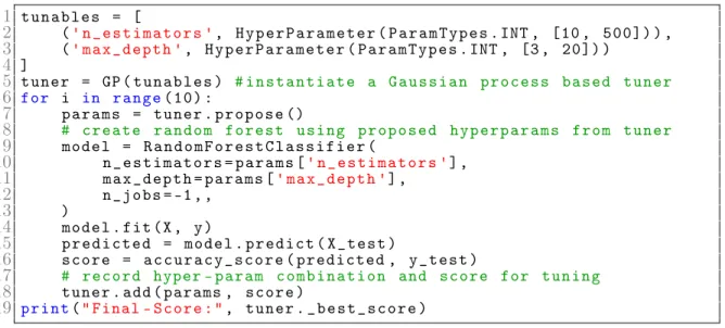
Figure 2-1: A Python code snippet illustrating how to use a tuner’s user API. The code illustrates how to use a tuner to tune a number of estimators hyperparameter between 10 and 500 and maximum depth of a tree between 3 and 20 for a random forest. The code snippet is given training data 𝑋, 𝑦 and testing data 𝑋𝑡𝑒𝑠𝑡 and 𝑌𝑡𝑒𝑠𝑡.

The tuner does not require the user to store any scoring data on their end. The user only has to call two methods after initialization, add to add new data to the tuner and propose to receive a new recommendation from the tuner.

devised by experts require numerical variables. An expert contributor would override the existing fit method to contribute a new meta modeling technique. An example would be fitting a Gaussian process to the hyperparameter score data.

• predict: An expert can override the predict function in order to use the meta-model to predict the mean score and standard deviation that would be given to a candidate hyperparameter combination. An example would be using the trained Gaussian process to predict the score of a given hyperparameter combination.

• acquire: An expert can override the acquire method in order to select which candidate to propose given a list of predictions (mean and standard deviation). Two examples would be returning the score with the highest predicted mean, or the one with the highest predicted expected improvement [28].

v v v v 12 22 21 11 22 21 12 11

[ ]

Figure 2-2: Interaction between the user API and developer-overridden methods for the tuner class add method.

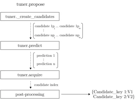
tuner._create_candidates candidate 1p ... candidate 1p 1 m candidate np ... candidate np ... 1 m prediction 1 prediction n {Candidate_key 1:V1 Candidate_key 2:V2} ... condidate index tuner.predict tuner.acquire post-processing tuner.propose

Figure 2-3: Interaction between the user API and developer-overridden methods for the tuner class propose method

Figures 2-2 and 2-3 show how the contributor-written methods integrate into the user-facing API for tuners.

Our design enables expert contributions in the following ways:

Flexibility in tuner design: Experts are allowed to contribute new meta-modeling technique. This is very important, because new techniques are constantly being developed and improved upon as the field of AutoML expands. Contributors are also given control of the acquisition function, which is used to propose a solution from a list of predictions. This is also very important, as there is little agreement in the AutoML expert community as to whether one function consistently outperforms another. Figure 2-4 shows how pairing a series of different modeling techniques and acquisition functions can create a series of different tuners. The choice of the Gaussian process (GP) meta-modeling technique versus the Gaussian copula process (GCP) breaks the tuners into two categories. (These ideas are implemented by modifying the tuner’s fit and predict method.)

The tuners are next split based on their acquisition function. The basic GP and GCP-based tuners use the maximum predicted score to determine which candidate to propose. The other tuners use maximizing expected improvement as the acquisition function. This is implemented in the tuner classes by overriding the acquire method. Finally, the tuners differ as to whether they include a concept of "velocity" along with the model, only favoring the trained model’s predictions over a uniform tuner if the velocity of the scores is large enough. The GPEiVelocity/GCPEiVelocity tuners include this concept, and GPEi and GCPEi do not. This concept is integrated in the tuner by calculating the velocity in fit. In predict, if the calculated velocity is not above a certain threshold, the model defaults to using a uniform tuner.

Handling data transformations: In this design, the expert contributors don’t have to worry about the hyperparameter data types. Most methods that experts want to contribute to require numeric data. We do data transformations and reverse transformations outside the core fit/predict/acquire methods, so that experts that choose to contribute to the methods don’t have to worry about how they are handled.

aquisition function (.acquire) aquisition function (.acquire) GPEiVelocityTuner GPEiTuner GPTuner GCPTuner expected improvement expected

improvement scoremax scoremax

Yes No

Gaussian

Process Gausian Copula_Process

GCPEiVelocityTuner GCPEiTuner

Yes No

Figure 2-4: Relationship between six different tuners. Includes the developer API functions overridden to implement the tuner.

2.2

Selector

A selector chooses from a set of discrete options by evaluating each of their past performances. Most implemented selector types use a multi-armed bandit technique to determine which option to select next. The selector API was established in the ATM paper, and was not modified during this thesis [29].

2.2.1

User API

• select: The user passes a dictionary to the selector’s select method. Each key in the dictionary corresponds to a choice available to the selector. Each value is a time-ordered list of scores achieved by this choice. The historical score data is first converted to rewards via the compute_rewards function. Next, bandit is called on the resulting historical rewards data in order to make a selection. The selected option for this time step is then returned to the user.

Table A.1 in Appendix A shows the methods a user would employ to create and use a selector object. The user only has to keep track of a dictionary mapping each of the choices to all of its corresponding scores. Figure 2-5 shows an example code snippet demonstrating how a user could use a selector. Because the choices are represented as keys of the dictionary, the user has a lot of flexibility as to which data type is used for

1

2 _{# Instantiate tuners}

3 rf_tuner = GP (('c', HyperParameter ( ParamTypes . FLOAT_EXP , [0.01 , ←˒

10.0]) ))

4 svm_tuner = GP ((' n_estimators ', HyperParameter ( ParamTypes .INT , ←˒

[10 , 500]) ))

5

6 # Create a selector for these two pipeline options

7 choice_scores = {'RF ': [], 'SVM ': []}

8 selector = Selector ( choice_scores . keys ())

9

10 for i in range( SELECTOR_NUM_ITER ):

11 # Using score data , use selector to choose next pipeline to ←˒

tune

12 next_pipeline = selector . select ( choice_scores )

13

14 if next_pipeline == 'RF ':

15 # give tuning budget Random Forest pipeline

16 for i in range( TUNER_NUM_ITER ):

17 _{params = rf_tuner . propose ()}

18 model = RandomForestClassifier ( n_estimators = params [' ←˒

n_estimators '])

19 model . fit (X, y)

20 rf_tuner . add ( params , accuracy_score ( model . predict ( ←˒

X_test , y_test ))

21 choice_scores ['RF '] = rf_tuner .y

22

23 elif next_pipeline == 'SVM ':

24 # give tuning budget to SVM pipeline

25 for i in range( TUNER_NUM_ITER ):

26 params = svm_tuner . propose ()

27 model = SVC (C= params ['c'])

28 model . fit (X, y)

29 _{svm_tuner . add ( params , accuracy_score ( model . predict (} ←˒

X_test , y_test ))

30 choice_scores ['SVM '] = svm_tuner .y

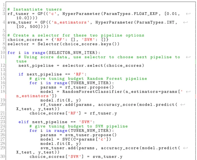
Figure 2-5: Python code snippet illustrating how to use a selector alongside a tuner to choose whether to next tune a random forest or an support vector machine (SVM) classifier. The n_estimators is a hyperparameter for a random forest and has the range [10, 500]. The c is a hyperparameter for SVM and has the range [0.01, 10.0]. The code snippet is supplied with training data 𝑋, 𝑦 and testing data 𝑋𝑡𝑒𝑠𝑡 and

𝑌𝑡𝑒𝑠𝑡. TUNER_NUM_ITER specifies the number of iterations of tuner when a particular

pipeline (in this case only a classifier) and SELECTOR_NUM_ITER specifies the number of iterations for the selector.

each of the choices. This allows for great flexibility on the user’s behalf, as they can represent the choices in whatever way they find most convenient.

2.2.2

Contributor API

When writing a new selector, there are three main methods a contributor would override. These methods and their desired functionality are described in Table A.2 in

Appendix A. The contributor can modify the bandit’s strategy to favor more recently chosen options, options with the highest velocity of reward, etc. The general selection methodology is as follows: First, the selector converts the scores into rewards, as determined by the compute_rewards function. Then, it calls bandit on the resulting choice reward combinations to propose a choice.

• compute_rewards: The compute_rewards method takes as its input a list of historical time-ordered score data and returns a list of rewards. The contributor can decide how the selection option scores correspond to the rewards. For exam-ple, if the distribution that the score comes from changes over time, it may not be optimal to consider old score data, as it is unlikely to accurately represent the current distribution. The contributor can then override the compute_rewards function to consider the rewards to be non-zero for only the most recent 𝑘 points. • bandit: In the bandit method, a dictionary is received that maps a discrete

choice to a list of rewards (the output of compute_rewards). The bandit method proposes a choice based on the rewards associated with each of the choices. • select: In the select method, the user passes a dictionary to the selector.

Each of the keys in the dictionary corresponds to a choice the selector can make, while the values consist of a time-ordered list of the scores that results from each choice. The historical score data is first converted to rewards via the compute_rewards function. Next, bandit is called on the resulting historical rewards data to make a selection. Finally, the method returns the selected option for this time step to the user.

Figure 2-6 shows how the contributor API interacts with the user-facing API for the select method. Contributors can decide how to pre-process the score data, how to convert the score data into the concept of a reward for the bandit, and which bandit function should be used.

pre-processing ... ... ... Option {Option 1: [score1 ... ] Option n: [score1 ... ]} {Option 1: [score1 ... ] Option 2: [score1 ... ] Option n: [score1 ... ]} {Option 1: [reward1 ... ] Option n: [rewardn ... ]} selector.compute_rewards selector.bandit selector.select

Figure 2-6: Interaction between user-facing API and developer overridden methods for selector class select method

Chapter 3

Recommender

Over the course of this thesis, we created a collaborative filtering-based search process from scratch. We call this a recommender, and describe it in detail in Section 3.3. We designed the API to closely match the tuner API in our library.

3.1

Overview of recommender problem

Suppose we have fitted a number of different machine learning pipelines on a number of datasets, and have recorded the resulting accuracy metric of each pipeline on each dataset. The knowledge gained about the performance of a particular pipeline on several datasets can, in some cases, be transferred to a new dataset.

For example, suppose there is a convolutional neural network that predicts whether a certain image contains an animal. Now, suppose we have the prediction problem of determining whether or not a certain image contains a dog. Because there is a similarity between the two problems, the architecture that performed best on the animal problem is likely to have high predictive accuracy for the dog problem. We can generalize this by leveraging the knowledge we have gained from running a series of machine learning pipelines in order to build a system which recommends a new candidate pipeline to try for a given unseen dataset.

3.1.1

Related Work

Multiple research groups have explored the topic of pipeline recommendation. Re-searchers at MIT have developed Delphi [11], a platform for machine learning that uses a distributed system for trying a series of pipelines and a recommender system to suggest a pipeline to the user. The recommender for Delphi uses a different methodol-ogy to make predictions than the one described in this thesis, as it does not use matrix factorization to reduce the space and sparsity of the matrix. The Delphi system is also not extensible, and the recommender methodology can not be changed.

In [14], the authors use probabilistic matrix factorization to infer the data missing from the matrix (including the new dataset for which they wish to propose a pipeline). The recommender acquires the predictions based on expected improvement, and the resulting system is tested on a matrix composed of various pipeline scores on a series of OpenML datasets. This recommender system is used in a series of experiments, and the work released pertains only to the results derived in the paper itself. This is a methodological contribution one which can be added to our open source and be made available to users.

3.1.2

Notation

In this section we will establish notations and naming conventions in use throughout the system. In the recommender system, the goal is to predict which of a candidate set of pipelines, whose hyperparameters are all fixed to certain values, will yield the highest accuracy score. Two pipelines can have the same steps, but may differ only by the hyperparameter values. For example, there can be two different pipelines, each of which use principal component analysis (PCA) on the input followed by a random forest, as long as the two pipelines have different hyperparameter values. This is because different hyperparameter combinations can yield dramatically different results when trained on the same dataset.

At the heart of the recommender system is the matrix that holds the known accuracy scores of given pipelines on given datasets. This matrix will be referred to as

the dataset pipeline performance matrix (dpp). In this matrix, each row represents a unique dataset and each column represents a unique machine learning pipeline. In the matrix, the value at row 𝑖 and column 𝑗 is the accuracy score (typically calculated using cross-validation) of pipeline 𝑖 tried on dataset 𝑗.1 If the pipeline has not been

tried on the dataset, the value is 0.

Now suppose we are given a new dataset for which we want a pipeline recommenda-tion. We will refer to this as d_new. For d_new we create a new row in the dpp matrix filled with zeros, to indicate that no pipeline has been tried. Throughout the recom-mendation process, we are consistently trying new pipelines on d_new and updating its row with the accuracy scores achieved by those pipelines. Each recommender object has only one d_new for which it recommends pipelines. The vector representation of the scores of the pipelines on d_new will be referred to as dpp-vector. Pipeline performance information is stored only in dpp-vector; the dataset is not represented as a row in dpp-matrix. In Section 3.3 we will describe the API, and in Section 3.2 we will describe the methods used for recommending.

3.2

Methods

Sparseness possess a huge problem for the recommender. Due to computational costs associated with fitting a pipeline to a dataset and evaluating it via cross validation, it is not feasible to try all of the possible pipelines on all of the known datasets. In fact, each dataset will only have been tried on a small subset of the pipelines, leading to very few non-zero entries in the dpp matrix. For example, in the matrix used in this chapter to demonstrate the efficacy of the recommender, we had a total of 9,384 unique pipelines, and each dataset was only tried on 363 of them.

If the dpp matrix were to make recommendations directly, the results would likely not be optimal, as the algorithm would probably only choose the dataset with the greatest number of pipelines that overlap with the ones that are tried on d_new,

1_{The score can be any metric, but for the purpose of this thesis it refers to the mean f1-score} calculated during cross validation.

regardless of the performance of these pipelines. We can solve this problem using matrix factorization (mf). Matrix factorization projects the matrix onto a lower-dimensional space, reducing the lower-dimensionality with the aim of reducing the sparsity. We can then compare the rankings of the values in the lower-dimensional space. Below, we present the current recommender we built.

Matrix factorization-based recommender

1. Use matrix factorization to reduce the dimensionality/sparsity of the dpp-matrix. We use non-negative matrix factorization [13, 8] to decompose dpp-matrix into a n-datasets×num-desired-componentsmatrix (dpp-matrix-decomposed) as shown:

dpp-matrix ≈ dpp-matrix-decomposed · 𝐻 (3.1) where 𝐻 is some num-desired-component𝑠 × num-pipelines matrix.

2. Gather data about pipeline performances on d_new in the form of dpp-vector. Similar to dpp-matrix, each column 𝑗 in the 1D vector represents the performance of the pipeline corresponding to that index on d_new.

3. Use the trained mf model to project dpp-vector on the the reduced dimensionality space yielding dpp-vector-decomposed. This can found by solving:

dpp-vector-decomposed ≈ dpp-vector · 𝐻−1 (3.2) Where 𝐻 is the matrix calculated in Equation 3.1, found during the fit process of the matrix factorization.

4. In the reduced space, find the matching dataset in dpp-matrix-decomposed that is closest to the dpp-vector-decomposed as determined by Kendall-Tau distance (ie greatest Kendall Tau Agreement). In case of a tie, choose at random from the tied options.

In order to find the closest matching dataset, we chose to compare the rankings of the pipelines between two datasets, as opposed to the closeness of performance scores. Because we used matrix factorization to reduce the sparsity of dpp-matrix and dpp-vector, we find the closest matching dataset and compare ranking in the reduced

space. NMF is known to have clustering-like effects, where each cluster is a column in the reduced space and the cluster membership is determined by whichever column has the largest value for the row [22]. By calculating the Kendall Tau agreement in the reduced space, we are essentially comparing the relative-rankings of the reduced pipeline (column) clusters for each dataset.

We compare rankings because we care about predicting the highest-performing pipeline rather than the actual score of this pipeline. The matching dataset may only compare relatively in score performance, as one of the datasets may be much harder to accurately classify than the other. We define the matching dataset as the dataset that has the highest Kendall Tau agreement [18]:

Kendall Tau agreement =

(number agreeing pairs − number non-agreeing pairs)

𝑛(𝑛 − 1)/2 (3.3)

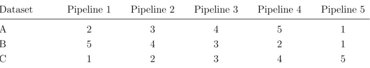
The higher the agreement is, the more that the two datasets agree on the compar-ative ranking of the pipelines. This is important because the actual projected values of the pipeline scores may have widely different ranges. Suppose we have 5 pipelines, numbered 1 through 5, along with 2 datasets, B and C. We are trying to find the dataset that most closely matches dataset A (which has been tried on pipeline 1 and 2). Suppose that dataset A is very similar to dataset C.

Table 3.1: Potential scores for three datasets A, B, C on 5 pipelines 1,2,3,4,5 Dataset Pipeline 1 Pipeline 2 Pipeline 3 Pipeline 4 Pipeline 5

A 0.5 0.6 0.7 0.8 0

B 0.9 0.7 0.8 0.6 0.5

C 0.5 0.6 0.7 0.8 0.9

Table 3.1 represents a matrix of potential scores for this scenario and Table 3.2 shows the corresponding rankings. For simplicity, we will not use matrix factorization, and will instead compare the rankings in the space of all five pipelines.

Table 3.2: Score rankings corresponding to table 3.1

Dataset Pipeline 1 Pipeline 2 Pipeline 3 Pipeline 4 Pipeline 5

A 2 3 4 5 1

B 5 4 3 2 1

C 1 2 3 4 5

B would match dataset A, as they agree 1 time and dataset C and A never agree. Under the Kendall-Tau agreement, however, we look at pairwise agreements. Dataset C and A agree on the following pairs:

• Pipeline 1 < Pipeline 2 • Pipeline 2 < Pipeline 3 • Pipeline 3 < Pipeline 4 • Pipeline 1 < Pipeline 3 • Pipeline 1 < Pipeline 4 • Pipeline 2 < Pipeline 4

giving a total of 6 agreements. Dataset B and A agree on the following pairs:

• Pipeline 1 > Pipeline 4 • Pipeline 2 > Pipeline 5

• Pipeline 3 > Pipeline 5 • Pipeline 4 > Pipeline 5

giving a total of 4 agreements. By the Kendall-Tau agreement, Dataset C is closest to Dataset A. Given the dataset pipeline results, Dataset C is clearly the better option, as the scores match perfectly for every pipeline other than Pipeline 5.

5. Compose a list of candidate pipelines for the new dataset made up of all untried pipelines on the dataset.

6. When making predictions, rank the pipelines based on their rankings for the matching dataset.

7. Acquire the predictions by choosing and proposing the pipeline with the highest ranking. In the case of a tie, chose at random from the options that tie.

3.3

Design

The recommender system attempts to find the best pipeline for a dataset, given a set of candidate pipelines. We have the following requirements:

dpp-matrix At the core of the recommender system is the dpp-matrix. This must be made available to the system. Each column of the matrix is a different pipeline and each row is a dataset. The value at 𝑖, 𝑗 is the accuracy score for pipeline 𝑗 on dataset 𝑖. It is up to the user to maintain some sort of data structure mapping the column index to the actual pipeline that it represents. This is a valid design decision, as the user must already possess knowledge about the pipeline that the column represents in order to create and fill in the recommender matrix or try a specified pipeline on d_new.

Same accuracy score: In order for the recommender system to work, the evaluation metric used for the score must be the same across all datasets. This is because the recommender system works by comparing the scores between different pipelines. If the evaluation metrics differ, the scores have different maximum and minimum values, making score-based ranking of pipelines impossible.

3.4

User API

The API for recommenders matches that of tuners as closely as possible, in order to keep the APIs consistent and because they are used similarly. Users will likely try each pipeline individually. Using the add method, users can incrementally add the score for each pipeline, rather than keeping track of all the data (pipelines and scores) and calling fit on everything. Table A.5 in Appendix A shows the recommender class methods available to users.

• add: The user passes a dictionary to the recommender. The keys in the dictionary are integers representing pipeline indices that the user has tried for their new dataset. The value is the accuracy score for that pipeline on their dataset. This method is very similar to the add method for a tuner. The recommender updates

1 #m = Matrix of dataset - pipeline - performances

2 _{# num_iterations = Number of iterations}

3 recommender = Recommender (m)

4 for i in range( num_iterations ):

5 pipeline_index = recommender . propose ()

6 score = result of trying pipeline index on dataset

7 recommender . add ({ pipeline_index , score })

8 best_pipeline_index = recommender . _best_pipeline_index

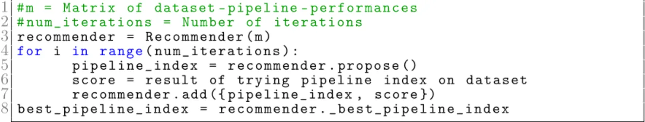
Figure 3-1: Python pseudo-code snippet illustrating how to use a recommender’s user API

its internal state with the new pipeline-score data and refits the meta-model on the new updated data. No external data storage is required on the user side.

• propose: The user calls propose to receive a new pipeline index proposed by the model that may improve the score. As with the tuner, the recommender first creates a list of candidate pipelines that haven’t yet been tried on the given dataset. It uses the meta-model to predict scores for each pipeline. Next, it uses the specified acquisition function to select which of these candidates to propose to the user. While this method involves a lot of computations, the API is kept easy-to-use for the user. It naturally fits into an iteration structure where the user can receive a pipeline index from the recommender, try it and score it, and then update the recommender with its score.

Figure 3-1 shows an example pseudo-code describing how the user would use the recommender system. As we can see, the API is very clean and easy for users to use. The user also has easy access to the best pipeline and its score, which are stored as class attributes. Minimal code is required on the user’s part in order to integrate a recommender system.

3.5

Contributor API

Table A.6 in Appendix A shows the recommender methods that contributors who wish to write their own recommender can override. As with the user API, the contributor API closely matches that of the tuner, so that experts who have contributed to one

type of object have a minimal learning curve when contributing to another. This also helps keep the library consistent. The following is a list of recommender methods that the contributor can override.

• fit: The contributor overrides the fit process to fit the meta-model to both the dpp-matrixdata composed of known pipeline and score combinations along with a vector of pipeline scores on d_new. We abstracted this functionality into its own method to match the general fit/predict API that is commonly used by machine learning libraries. This way, contributors can simply implement their meta-modeling technique as a model and call model.fit in the recommender API. One example would be fitting a matrix factorization model to the dpp-matrix and using that to reduce the dimensionality of both the dpp-matrix and the pipeline-performance vector of d_new.

• predict: The contributor overwrites the predict function to use the meta-model to rank a series of candidate pipelines. As with .fit, we abstracted predictto its own function to match the scikit-learn practice of calling model.fit and model.predict. The contributor uses their meta-model to make predictions. An example would be using the relative rankings of the dataset whose pipeline scores most closely match the d_new. We chose to have the predict function rank the candidates rather than assigning them a raw score, because while similar problems may be useful for predicting relative performance, they are less likely to accurately predict the true numerical performance of a pipeline on a dataset.

• acquire: The contributor overwrites the acquire method to select which candidate to propose given a list of predictions. An example would be returning the pipeline that ranks the highest according to its prediction.

Similar to the tuner, the public methods add and propose are fixed and not meant to be overridden by contributors. This is because they include data processing and other nuances abstracted away from the contributor. The API for the contributor

pre-processing

[score_0, 0, score_2] {pipeline-index 0: score_0

pipeline-index 2: score_2}

recommender.add

Figure 3-2: Interaction between user API and developer-overridden methods for recommender class add method

recommender._get_candidates [candidate-1 ... candidate-n] [ prediction-1 ... prediction-n] pipeline-index candidate-index recommender.predict recommender.acquire post-processing recommender.propose

Figure 3-3: Interaction between user API and developer-overridden methods for recommender class propose method

is designed to be as simple as possible. The contributor deals only with an array of scores for fitting. Figures 3-2 and 3-3 show how those methods that a contributor can override interact with the methods that the user calls for a recommender.

The contributor does not have to override all of the methods. The default get_candidates and acquire functions are likely sufficient for most recommenders. The default get_candidates returns all pipelines that haven’t yet been tried on the new dataset. The default acquisition function returns the index corresponding to the maximum ranking. At a minimum, contributor should override fit to specify how the model should be fit to the dpp-matrix, and predict to specify how it should use the fitted model to rank different pipelines.

3.6

Evaluation

We evaluate the mf-based recommender against a uniform sampling method that proposes a pipeline chosen at random from the candidate list of pipelines for each iteration.

3.6.1

Data

Creation of dpp-matrix: In order to generate the dataset-pipeline performance matrix, we used data gathered by a series of ATM runs using grid search to find the best pipeline for many different datasets2_{. 420 datasets were used in this experiment.}

Each dataset was run on roughly 600 different pipelines 3_.

The data from these runs was stored in four csv files. The schema of these csv files is described in the documentation here: https://github.com/HDI-Project/ATM/blob/ master/docs/source/database.rst.

In the raw ATM results file, the pipeline information was stored as in a string with the model type (eg SVM, random forest) and all of the hyperparameter values for the model. We first aggregated all of the pipelines by model type and hyperparameter configuration. This helped us identify 19,389 unique pipelines. We assigned each unique pipeline an index and then grouped the pipelines by dataset ID. There were 286,577 dataset-pipeline runs to begin with.

We further reduced the pipelines to a subset consisting of ones that ATM currently supports, so that when a specification of the pipeline is given, we are able to learn a model and predict using scikit-learn. We ended up with 9,384 pipelines.

After this selection, we found that each of the 420 datasets had been tried on an average of 363 different pipelines. We mapped each dataset ID to a list of pipelines and scores. From there, we constructed the dpp-matrix by filling in dataset and pipeline performance pairs of the dpp-matrix. Where the dataset-pipeline performance is unknown, the matrix is filled in with zeros.

2_{The raw data from the runs is available at https://s3.us-east-2.amazonaws.com/atm-data-store} 3_{We are calling these pipelines, but they only consisted of a classifier}

Ultimately, the matrix we have constructed is about 96% sparse, as each dataset has been tried on approximately 4% of the pipelines. This matrix is publicly available at https://s3.amazonaws.com/btb-data-store/recommender-evaluation/dpp-matrix/ Evaluation datasets: We subselected a set of 30 datasets. Table 3.3 gives the list of these datasets. For each of these datasets, we will make recommendations and evaluate the performance of the mf-based recommender system.

Table 3.3: List of datasets used in evaluation of matrix factorization-based recom-mender.

Dataset Name Dataset Name

mf_analcatdata_asbestos_1 analcatdata_bankruptcy_1 AP_Endometrium_Prostate_1 auto_price_1 breast-tissue_1 chscase_health_1 diggle_table_a1_1 fri_c0_100_10_1 fri_c1_100_25_1 fri_c1_100_50_1 fri_c2_100_25_1 fri_c2_100_50_1 fri_c4_100_25_1 fri_c4_100_50_1 fri_c4_100_100_1 fri_c4_250_100_1 humandevel_1 machine_cpu_1 meta_batchincremental.arff_1 meta_ensembles.arff_1 meta_instanceincremental.arff_1 pasture_1 pasture_2 pyrim_1 rabe_166_1 sonar_1 visualizing_ethanol_1 visualizing_slope_1 fri_c0_250_50_1 witmer_census_1980_1

Experiment Setup: With the dpp-matrix and evaluation datasets at hand, we evaluate a mf-based recommender as follows:

1. We choose 30 random datasets (named in Table 3.3) as our candidate datasets, for which we want to find the best possible pipeline4.

2. For each dataset, we:

4_{The train-test splits for these datasets are available at https://s3.us-east-2.amazonaws.com/} atm-data-store/grid-search/

(a) Remove the row corresponding to this dataset from the dataset-pipeline performance matrix. We pretend that this is a new dataset, d_new. (b) Use the remaining matrix to fit a recommender model.

(c) Use the recommender to propose a pipeline index for this dataset.

(d) Based on the pipeline index, get the string representation of the pipeline. Parse this to create and train a machine learning model on the dataset using ATM’s Model class.

(e) Score the model based on the mean f1-score from 5-fold cross validation. (f) Add the score to the matrix at the 𝑖, 𝑗 location, where 𝑖 corresponds to the

dataset index and 𝑗 is the pipeline index.

3. Continue repeating steps (a) through (e) until we have proposed and evaluated 50 pipelines. These correspond to 50 iterations.

4. Store all of the recommendation/score data for later evaluation.

Together, steps 2, 3, and 4 make up one trial. In order to assure confidence in the results and assess statistical significance, we run 20 trials on each dataset. Each experiment is made up of 20 trials run on a particular dataset.

3.6.2

Storing the results

We record the results of the experiments for each dataset-recommender pair in a separate csv file. The first row in the csv file is the first pipeline proposed by the recommender for an experiment. The second row is the resulting average f1-score of this pipeline on the dataset after 5-fold cross validation. The third row is the standard deviation of the f1-score for the pipeline calculated from the cross-validation. The columns continue in this manner for each of the trials. Each row in the csv represents an iteration along with the results for all of the trials at that iteration. Table 3.4 shows how this csv format translates into a table of results. Storing the results in this format means that we can easily use the Pandas Python library [20] to turn the CSV

file into a DataFrame for computations. As we are storing the mean and standard deviation of the f1-score for each pipeline on the dataset, we have a lot of flexibility around how we analyze and use the results.

Table 3.4: Storage of Results of recommender Evaluation

trial_0_ pipeline_ index trial_0_ mean_f1 trial_0_ std_f1 trial_20_ pipeline_ index trial_20_ mean_f1 trial_20_ std_f1 trial_0_ pipeline_ index_ iteration_0 trial_0_ mean_f1_ iteration_0 trial_0_ std_f1_ iteration_0 trial_20_ pipeline_ index_ iteration_0 trial_20_ mean_f1_ iteration_0 trial_20_ std_f1_ iteration_0 trial_0_ pipeline_ index_ iteration_ 50 trial_0_ mean_f1_ iteration_ 50 trial_0_ std_f1_ iteration_ 50 trial_20_ pipeline_ index_ iteration_ 50 trial_20_ mean_f1_ iteration_ 50 trial_20_ std_f1_ iteration_ 50

We use a standard naming scheme of recommender-typ_dataset-name_results.csv to make it easy to find the results for a specific experiment. The results are stored in a public S3 bucket 5_{. This open-sources our results, and allows others to use the data}

that we have generated for their own experiments.

3.6.3

Evaluation of Results

We compare our matrix factorization recommender against a uniform recommender that proposes each pipeline with equal probability.

For an experiment on a dataset 𝑑 that has a recommender 𝑟, we define the best-so-far metric pbesti𝑑, or the score of the best-performing pipeline by iteration

𝑖 as: pbestid = ∑︁ 𝑡 𝑚𝑎𝑥0≤𝑗≤𝑖𝑓 (𝑝𝑡𝑖, 𝑑) 𝑡 (3.4)

where 𝑓(.) is the cross-validated accuracy score when pipeline 𝑝𝑡

𝑖 is evaluated on

dataset 𝑑. The accuracy metric used in our experiments is f1-score. 𝑝𝑡

𝑖 is the pipeline

proposed by the recommender at iteration 𝑖 in trial 𝑡 for this dataset. Thus, pbesti𝑑

gives the best score achieved by the recommender at iteration 𝑖, averaged across all the trials.

Evaluation Metrics

In order to compare two recommender methods, we compare their pbesti𝑑 scores

using a series of metrics.

• Average pbesti𝑑 at iteration 5, 10, 25, 50: We take the mean of all the

experiments (across different datasets) for each recommender type. Because the same accuracy metric (in our case, the f1-score) is used across datasets, this average effectively compares the overall performances of the two recommenders. • Wins for average pbesti𝑑 at iteration 5, 10, 25, 50: We also count the

number of time that each method “won.” To do this, we take each dataset at a specified iteration, check which pbesti𝑑 is higher, and simply tally the "wins"

for each method.

• Average percentage difference in pbesti𝑑 at iteration 5, 10, 25, 50: In

addition to comparing the mean pbesti𝑑, we also calculate the mean

percent-age difference in pbesti𝑑, in order to quantitatively measure any performance

increase. This metric enumerates any potential performance gain that would result from using a matrix factorization recommender instead of a uniform recommender. We calculate the percentage difference in pbesti𝑑 for a dataset

between uniform and matrix factorization recommender (1 − mf-pbesti𝑑

uniform-pbesti𝑑), and

then average over all datasets.

• 90% Confidence interval around average pbesti𝑑 for iteration 50: By

leveraging the scores from all of the trials, we can calculate a 90% confidence interval around the calculated pbesti𝑑 at iteration 50 for a given dataset. We