HAL Id: hal-02974933
https://hal.archives-ouvertes.fr/hal-02974933
Submitted on 22 Oct 2020
HAL is a multi-disciplinary open access
archive for the deposit and dissemination of
sci-entific research documents, whether they are
pub-lished or not. The documents may come from
teaching and research institutions in France or
abroad, or from public or private research centers.
L’archive ouverte pluridisciplinaire HAL, est
destinée au dépôt et à la diffusion de documents
scientifiques de niveau recherche, publiés ou non,
émanant des établissements d’enseignement et de
recherche français ou étrangers, des laboratoires
publics ou privés.
a Process-Based State Space rather than a Potential
Surface
Cédric Gaucherel, F. Pommereau, Christelle Hély
To cite this version:
Cédric Gaucherel, F. Pommereau, Christelle Hély. Understanding Ecosystem Complexity via
Appli-cation of a Process-Based State Space rather than a Potential Surface. Complexity, Wiley, 2020, 2020,
pp.1-14. �10.1155/2020/7163920�. �hal-02974933�
Research Article
Understanding Ecosystem Complexity via Application of a
Process-Based State Space rather than a Potential Surface
C. Gaucherel ,
1F. Pommereau,
2and C. H´ely
31AMAP-INRAE, CIRAD, CNRS, IRD, Universit´e de Montpellier, Montpellier, France 2IBISC, Universit´e d’Evry, Evry, France
3Institut des Sciences de l’´Evolution de Montpellier (ISEM), EPHE, PSL University, Universit´e de Montpellier, CNRS, IRD, Montpellier, France
Correspondence should be addressed to C. Gaucherel; [email protected] Received 19 June 2020; Accepted 18 September 2020; Published 6 October 2020 Academic Editor: Tomas Veloz
Copyright © 2020 C. Gaucherel et al. This is an open access article distributed under the Creative Commons Attribution License, which permits unrestricted use, distribution, and reproduction in any medium, provided the original work is properly cited. Ecosystems are complex objects, simultaneously combining biotic, abiotic, and human components and processes. Ecologists still struggle to understand ecosystems, and one main method for achieving an understanding consists in computing potential surfaces based on physical dynamical systems. We argue in this conceptual paper that the foundations of this analogy between physical and ecological systems are inappropriate and aim to propose a new method that better reflects the properties of ecosystems, especially complex, historical nonergodic systems, to which physical concepts are not well suited. As an alternative proposition, we have developed rigorous possibilistic, process-based models inspired by the discrete-event systems found in computer science and produced a panel of outputs and tools to analyze the system dynamics under examination. The state space computed by these kinds of discrete ecosystem models provides a relevant concept for a holistic understanding of the dynamics of an ecosystem and its abovementioned properties. Taking as a specific example an ecosystem simplified to its process interaction network, we show here how to proceed and why a state space is more appropriate than a corresponding potential surface.
1. Introduction
Most ecologists would admit that ecosystems are complex, although some might appear simple. Ecosystems appear to form emergent structures (e.g., [1, 2]), exhibit nonlinear properties (e.g., [3, 4]), and be clearly out of equilibrium (e.g., [5, 6]). Moreover, the fact that most ecosystems today strongly interact with society and contain several human groups heightens this feeling of complexity [7, 8]. Yet, most studies focus on just some components of the ecosystem, either biotic (e.g., species community), abiotic (e.g., climate, element cycles), or anthropic (ecosystem services), and a definitive demonstration of integrated ecosystem complexity is still lacking. In addition, most analyses focus on com-plexity at a specific time, often concentrating on patterns rather than on long-term dynamics [1, 9]. In this conceptual paper, we propose a detailed methodology for the long-term study of ecosystem dynamics and for qualifying their complexity using process-based models.
Ecosystem complexity is derived first and foremost from the combination of biotic, abiotic, and human components which also form a tangled web of continuous interactions [10–12]. Some socioecological systems seem quite simple, with few components and few processes, but these cases remain scarce. Theoretical ecologists with a true interest in the whole (socio)ecosystem, not just some parts of it, have spent decades debating ecosystem dynamics and their sta-bility or resilience [3, 13]. Whether a potential function or a resilience surface [14–17], synthetic and conceptual models should be able to fit any specific trajectory observed in the ecosystem under study. The recent nature of ecology as a discipline and mostly partial and short-term observations provide us with a limited view of ecosystems. As a result, such models often focus on short-term dynamics and mainly on pattern analyses [9, 18, 19]. Models of complexity in ecology thus remain phenomenological. For this reason, even partially validated process-based models of ecosystems offer a promising opportunity to produce understandable,
Volume 2020, Article ID 7163920, 14 pages https://doi.org/10.1155/2020/7163920
robust long-term dynamics. Here, we intend to review the mainstream models of ecosystem dynamics, to demonstrate some of their limitations, and finally, to provide a process-based methodology that will hopefully bypass such limitations.
When studying or managing an ecosystem, be it tem-perate or tropical, terrestrial or aquatic, natural or anthropic, a suggested preliminary step is an exhaustive understanding of its overall dynamics. Practically speaking, ecologists today investigate whether or not a specific ecosystem studied is stable [3, 4], resilient [2, 20], and moreover how far from any tipping points or catastrophic shifts it lies [21–23]. Physics has long provided powerful tools for these objectives with regard to physical systems. For example, physical models often provide ordinary differential equation (ODE) systems and summarize the most probable dynamics (and sharp changes) into phase spaces and potential functions [24, 25]. Such syntheses then enable confident predictions of future system states, to prevent unwanted states and advise on expected states.
Despite recent attempts, such synthetic models for ecosystems are still lacking. Some theoretical models have been proposed [26–29], but they rarely fit and accurately calibrate observations, or if so, rarely study more than one state variable (e.g., biomass and/or annual rainfall). In ad-dition, such models are probabilistic in essence, whereas possibilistic models would afford exhaustive exploration of complex (eco)system dynamics. Here, our first and most important objective is to provide ecologists with a new conceptual framework for achieving this goal of exhaustive computation of any ecosystem dynamics [30, 31], and to simultaneously illustrate the approach in a complex case study. Moreover, the mainstream models used today in ecosystem ecology still suffer from several limitations [32]. Our second objective is to list and debate these chief limitations.
For this purpose, we recently developed an original type of models [18, 30], based on the discrete event and qualitative
systems commonly used in theoretical computer sciences
[33–35]. Here, we will illustrate the approach with a qual-itative Petri net in the case of an insect (termite) colony [36], which is presumed to mimic an ecosystem undergoing abrupt qualitative change, and potentially experiencing strong long-term disturbances. We will show how the qualitative state space (sometimes called the reachability or labeled transition space) of the modeled insect colony provides a relevant synthesis of this ecosystem’s dynamics. Finally, we will analyze this state space to verify that it is not subject to the same limitations as identified in other eco-logical models, and to suggest future directions.
2. State Space of a Qualitative Ecosystem
Here, we propose an original model intended to represent the overall dynamics of any complex (socio) ecosystem. The proposition states that it is possible to exhaustively capture overall ecosystem behavior on the basis of a qualitative, discrete, and integrated description of its interactions [18]. The interactions within a given ecosystem are all the relevant
processes involved in the system dynamics, hence the process-based model. This kind of discrete model has already proved useful, and interested readers may refer to papers describing the mathematical details of the method and some applications [30, 37, 38]. In the present study, we illustrate such an approach with the specific case of a simplified theoretical insect colony. This termite colony is assumed to mimic a typical ecosystem comprising biotic, abiotic, and anthropogenic-like (the farming termites) components [36], as well as all their associated (i.e., bioecological, physico-chemical, and socioeconomic) interactions. The output from the model consists in a discrete qualitative state space of the ecosystem, grouping all the states that the ecosystem may potentially reach from an initial state and thus all its trajectories.
We chose to model eusocial insect colonies for the reasons that they experience drastic change (tipping points, TPs) over time, but any other ecosystem-like models may be used (Figure 1(a)). We chose to work on Macrotermitinae termites [36] which, like some ant species, construct large colonies (up to millions of inhabitants), [39] sometimes considered as super-organisms with complex functioning. These termites cultivate fungi in special chambers, build aerial structures (called mounds) to improve air circulation, and divide their nests into a royal chamber, fungus cham-bers, and egg rooms (Figure 1(a)). Given the ability of this eusocial species to develop food production, termites might also be considered as mimicking humans (farmers) in agrosystems.
One way of conceptualizing the ecosystem under in-vestigation is to represent it as a graph (i.e., network) of components connected by processes, the interaction net-work, whatever the interactions (Figure 1(b)). The model is fully qualitative (Boolean) and allows components to be present or absent only. The resulting ecosystem graph is then manipulated using a rigorous model based on a discrete Petri net to formalize any change in the topology of this graph (i.e., the neighboring relationships between present com-ponents). Developed in computer science [31, 35], Petri nets are commonly used in biology (e.g., [40, 41]) and are powerful tools for rigorous formalization of changes in network topologies occurring during system dynamics. Such Petri nets are radically different from traditional ecological models based on ODE equations (e.g., [2, 4]) in that they deal with topological changes in interactions during the simulation rather than dynamics carried by a fixed topology. Our approach might be closer in spirit to other attempts, such as Richard Levins’ “loop analysis” dedicated too linear systems and its most recent versions of qualitative models [42].
Discrete-event models provide state space outputs that can be readily analyzed to highlight relatively stable (or resilient) dynamics, tipping points, and any other specific trajectories. Such state spaces show similarities with the state-and-transition models that have proved useful in modeling ecological succession [43], except that our state spaces are deduced from predefined processes instead of being directly drawn from observations. Hence, such models are possibilistic models as they exhaustively explore the
possible dynamics of the (eco) system, and differ strongly from traditional probabilistic models in ecology [17, 44]. It appears crucial to identify all possible trajectories to un-derstand the overall ecosystem dynamics, rather than fo-cusing on the most probable trajectories.
In this kind of framework, any ecosystem can be rep-resented as a graph, in which every material component of the ecosystem (e.g., a termite population stage, fungi, air, and water) is represented by a node, with two Boolean states: “present” (the component is functionally present in the system and it may impact other components, also denoted as “+” or On) or “absent” (functionally absent from the system or “−” or Off). So, any state of the system is defined by the set of “+” and “−” nodes (Figure 1(b)). Any physicochemical, bioecological, and/or possibly socioeconomic process is translated into a Petri net rule, which describes the condition to be fulfilled, and the realization to be executed in such a case. Since the rules modify node states, the entire system shifts from one state to another through the discrete suc-cessive application of rules [30]. Rules progressively produce the state space, which provides the set of all system states reachable from the initial state and by the defined rules (Figure 2). This is easily translated and computed by any Petri net engine [35, 45].
The Petri net of the termite colony provides a highly instructive state space [30]. The termite modeling reaches
only 109 states (of 212possible states, approx. 2%), so we can
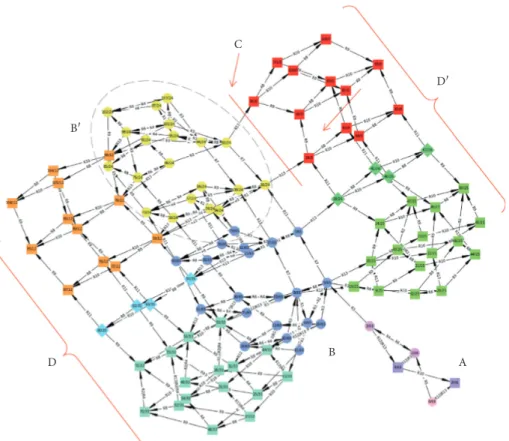
draw the exhaustive state space to visualize it (Figure 2). For larger systems, analysis can be performed automatically and without drawing the state space [37]. The state space graph displayed here is composed of several (colored) structures,
which we will further describe and interpret in ecological terms: the initial state (numbered 0, and represented by a hexagon, Figure 2-A), two topological structures usually called strongly connected components (SCCs, defined as a set of system states in which every state may be reached from any other state of the SCC, Figure 2-B and B′), and a number of decisive paths (e.g., irreversible ecosystem trajectories and tipping points, Figure 2-C), ultimately leading upward to basins and their associated deadlocks (states from which no other state is reachable, Figure 2-D and D′, squares). Hence, the state space provides a convenient, precise summary of the system’s behavior, its dynamic features, and all its possible qualitative trajectories.
From this state space, it is possible to compute a merged
state space automatically aggregating all the states of the
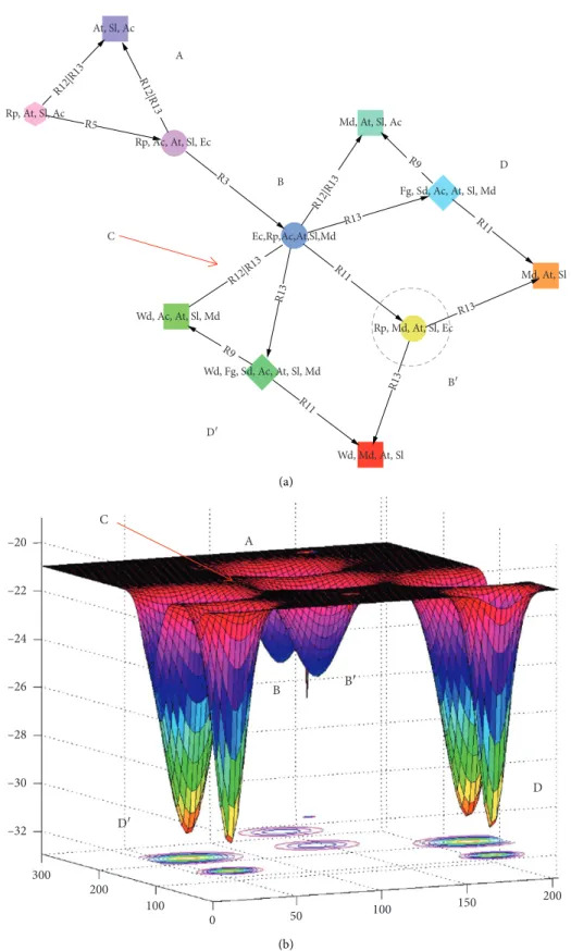
topological structures mentioned previously (Figure 3(a)). In this merged space, the SCC properties conveniently capture the ecosystem’s structural stabilities, that is, the number of states and the trajectories that qualitatively connect them (e.g., Figure 2-B). Tipping points are also visible as the successive rules (Figure 2-C and 3(a)-C) shifting the system from structural stabilities (e.g., B or B′) to deadlocks (e.g., D or D′), here meticulously identified and listed [30]. Other possible features (e.g., basins connecting the previous features) and ecosystem collapses (deadlocks) may also be computed and displayed on the same state space. Such topological analysis is usually accomplished on state spaces with as many as millions of states, in more complex and/or realistic ecosystem models [37, 38].
From this merged state space, we can then compute a potential-like surface (Figure 3(b)), referred to hereinafter as
Royal cell Nursery galleries Fungus gardens Chimney Ventilation shaft Nest Mound Soil (a) Structure Inhabitants Environment Competitors Resources Ec Fg Ac Rp Sd Wd Wk Md Ai At Te Sl (b)
Figure 1: Graphic of a termite colony (a) and its simplified interaction network (b). Termites modify their environment and build a mound with various chambers to host the colony (a). The original ecosystem graph is composed of 12 nodes (Table 1) with five colors representing their different natures (b, left). Their 15 associated interactions (i.e., processes, Table 2) are shown directionally (b) from component conditions to realizations.
the computed potential surface to distinguish it from other
traditional surfaces used in ecology and elsewhere
[14, 17, 25]. While stabilities may be represented by wells (e.g., Figure 3(b)-B), tipping points are represented by ridges connecting these wells (e.g., Figure 3(b)-C), and deadlock states or sets of states are represented by assigning them a virtually infinite depth on the computed potential surface (e.g., Figure 3(b)-D), so that the system can no longer escape from them. For this purpose, we linked the width, depth, and location of each topological feature with the number of states, the number of trajectory steps, and the path con-nections of each feature. This representation is intended to consider different components of resilience, namely, lati-tude, resistance, and precariousness [17]. For example, structural stability B′ involves 20 states, with a maximum of three steps required to leave it, and is irreversibly connected to B (Figure 4(a)). In this way, we built a surface that appears comparable to the traditional potential-like surfaces: yet, we highlight in the next section how different it is, once interpreted on the basis of the concepts supporting the qualitative discrete-event models used for this computation. The state space concept provides an easy way to identify structural stabilities, tipping points, and hysteresis. We stress that such topological features do not correspond perfectly to
the so-called dynamics (i.e., with these names) in ODE models, as the system here shifts sharply from one set of discrete qualitative states to other discrete qualitative states and could theoretically stay indefinitely in each of them. When the system remains stuck in a specific structural stability (e.g., B and B′ in Figure 2), all the states of such a stability are by definition connected through specific paths. The modeled ecosystem shifts from one state to the others through differentiated trajectories and then potentially comes back to the same state (Figure 4(a), blue and green arrows). These trajectories are numerous, with highly dis-tinctive paths in terms of ecosystem composition (the present components) or other properties. For example, it is possible to plot such hysteresis as a function relating the number of ecosystem components present to the number of steps required to reach the states (Figures 4(b) and 4(c)).
Many other properties are available and often quanti-fiable in the state space. It is relevant to use these trajectories to characterize the structural stability (e.g., B′ in Figure 4(a)), for example, by assigning it a “depth” defined by the maximum number of discrete steps required to reach the stability boundary and ultimately leave it (state colors) and representing the resistance [17]. The state space gathers as much information on transitions as on states, as it is possible
A C B D′ D B′
Figure 2: The full state space (or marking graph) of the termite colony model. The state space comprises 109 states labeled with a pair n/s where n is an identifying number for the marking and s is the number of strongly connected components (SCCs) for the basin or deadlock it belongs to. The initial state is displayed as a hexagon (A), deadlocks (states leading to a terminal state with no successor) are displayed as squares (five in total, of which two are in zones D and D′, and one (A) is close to the initial state), an example of two tipping points is displayed as a red segment (C), while other states are displayed as circles. Each SCC or basin is highlighted using a separate color (e.g., SCCs B and B′ are drawn in orange and green). The edges are directed and labeled with the number of the rule that was applied to perform the transition (defined in Table 2).
A C B D′ D B′ At, Sl, Ac R12|R13 R12|R13 R12|R13 R12|R13 Rp, At, Sl, Ac R5 Rp, Ac, At, Sl, Ec R3 Wd, Ac, At, Sl, Md Wd, Fg, Sd, Ac, At, Sl, Md Ec,Rp,Ac,At,Sl,Md Rp, Md, At, Sl, Ec Fg, Sd, Ac, At, Sl, Md Md, At, Sl Wd, Md, At, Sl R13 R13 R13 R13 R11 R11 R11 R9 R9 Md, At, Sl, Ac (a) B D′ D B′ C A –20 –22 –24 –26 –28 –30 –32 300 200 100 0 100 150 200 50 (b)
Figure 3: From the merged state space (a), it is possible to draw a tentative potential-like surface (b). In the merged version (a) of the full termite state space (Figure 2), each SCC and basin has been reduced to a single node and redundant paths have been removed. Nodes representing SCCs or basins (i.e., aggregate states) are noted (s) (circles) and labeled with the components present in all their states. From this reduction of the state space, specific paths leading to the main ecosystem collapses (squares), and highlighting the sharp transitions between them, can be more easily identified. For the potential surface (b), each structural stability (SCC, e.g., B and B′) has been represented as a well with a width corresponding to its number of states and a depth corresponding to the maximum number of steps for escaping it. The deadlocks (e.g., D and D′) are bottomless wells and are connected to other topological features with a continuous surface and sometimes through tipping points (C) (red arrow). We explain in the main text why such a representation is fallacious, though.
to analyze which process (interaction) is responsible for which transition between states or sets of states. For ex-ample, the ecosystem shifts drastically from stability B′ toward deadlock D′ through a TP (Figure 3(a)-C, red arrow). It is possible to compute a similarity index between all pairs of states or topological features to estimate the TP magni-tude. For example, a Jaccard index based on the present and
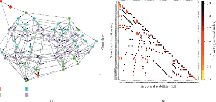
absent components would quantify the similarity between successive states. As an illustration, we computed this similarity index in a more complex wetland socioecosystem modeled in the same way (Figure 5(a)) [38] and automat-ically identified TPs such as the transitions entering dead-locks n/s 0 and 3 that were highly different from those seen previously (Figure 5(b), the two first columns of the matrix).
B′ (a) T o ta l no de n u m b er 5 4 3 6 8 1 2 7 9 0 Trajectory (steps) 5 6 7 8 9 10 11 Backward Forward 71-86-91-94-95-98-103-92-11-25/25-26-49-71 (b) 0.5 1.0 0.0 1.5 2.0 2.5 3.0 3.5 4.0 Trajectory (steps) 71-86-91-94-25/25-26-49-71 11 10 9 8
Total node number 7
6
5
Backward Forward
(c)
Figure 4: Illustration of the hysteresis found in the termite ecosystem state space (a), highlighting two specific trajectories (b). The structural stability displayed is B′ (Figures 2 and 3), composed of 20 states (a) labeled with a pair n/s where n is an identifying number and s is the number of discrete steps needed to exit the B′ stability (from 0 for states defining the boundary to 3 for the maximum number of steps to reach the boundary). The edges are directed and labeled with the number of the rule that was applied to perform the transition (Table 2). One specific cycling trajectory has been chosen in the B′ stability (a) (blue and green arrows), and this hysteresis is highlighted in the plane (number of present components versus discrete steps, b left). A second trajectory is displayed in the same plane (b right) to highlight the fact that many trajectories in the state space may exhibit hysteresis.
3. Comparison of the State Space with the
Potential Surface
A process-based model such as the present model of a termite ecosystem may provide some insights in ecology. In recent years, a growing body of studies in ecology has promoted the con-ceptual view of (socio)ecosystem functioning that we refer to here as the potential surface (Figure 4(a)). Although it has sometimes been called by other names, the principle remains the same: this metaphor suggests considering any ecosystem as a ball rolling down onto a hypothetical landscape made up of a surface in a higher dimension space [15, 17]. This (hyper)surface concept is borrowed from physics, where many systems have been shown to change according to a potential parameterized by intrinsic (e.g., state variables) and extrinsic variables (e.g., en-vironmental conditions) [24, 25]. There is no doubt that this concept is a convenient one for use in ecology too [44, 46]. This conceptual model is phenomenological, in that it potentially describes patterns in observation and is not based on knowledge of the underlying mechanisms. Metaphors are often slippery and it remains to be demonstrated that the potential as a concept is appropriate to ecosystem dynamics and to environmental processes (e.g., climatology [21, 22, 47]) in general. This section lists five possible criticisms of the potential metaphor.
3.1. Vertical Force. One critical assumption of the potential
analogy concerns the gravitational force that constrains movements on the surface. For the system to be located
above a certain elevation assumes the energy is higher than below that elevation due to the scalar field in which the system is immersed. Does such a force exist in ecosystems? And if yes, what is the nature of this force? Indeed, if the potential surface is such an easy-to-handle metaphor, it is undoubtedly due to the restoring torque that drives the ball along to the potential surface [15]. In physical systems, any potential is the origination of a force and is directly linked to energy [11, 48]. This force is often gravity but may also be associated with electrical or chemical potentials. In eco-logical systems, to our knowledge, no force or energy has been identified or analyzed, even when living systems tend to maintain their activity, for example, by homeostasis [49]. It is even harder to imagine what the nature of this force or these processes might be, considering that ecosystems are simultaneously physical and biological (and anthropogenic) objects.
A simple thought experiment might help in under-standing what is at play in this force, if anything. Take a simplified ecosystem such as vegetation in arid areas. In the absence of rainfall (the environmental conditions, say rainfall R), there is no vegetation (the state variable, biomass B) present, even on fertile soil. The absence of such variables (B, R) � (0, 0) may be, and usually is, considered a stable state [28], even with a system showing stochastic noise. In other words, the potential surface concept would plot the eco-system as a ball that has “fallen deep into” a well [44]. Now, let us push the system toward slightly wetter conditions and the emergence of vegetation. How would ecologists think the 1 2 3 6 Chr ono log y (a)
Structural stabilities (id)
Si mila ri ty ( Jacq ua rd index) 0.9 0.8 0.7 0.6 0.5 0.4 0.3 St ruc tura l st ab ili ties (id) (b)
Figure 5: Example of a more realistic socioecosystem analyzed using a discrete qualitative model, viewed by its merged state space (a) and its tipping points (b). The state space of this wetland socioecosystem (a), a temporary marsh with pastoralism [38], should be read downward, from the initial state (pink hexagonal node on top) to the terminal structural stability (red bottom node). Different stabilities (colors and identifiers) are connected through processes (i.e., edges as directional arrows) mimicking qualitative transitions between distinct states of the socioecosystem being modeled. The similarity between these successive states (in terms of present components) may be quantified using a Jaccard index (b) (hot colors) and plotted in a connectivity matrix grouping together all the structural stabilities reached by the ecosystem. Transitions exhibiting the lowest Jaccard index values between highly different states clearly identify the ecosystem’s tipping points (b) (left column).
ecosystem would behave? Would the system stay in this (putative stable) state with very little vegetation and rainfall? Will it gradually increase the biomass, form vegetation patterns, and start storing as much water as possible? Or will it simply revert to the previous state, with no vegetation and no more water?
The potential surface provides one (the?) answer. Due to the metaphoric gravitational force in the landscape, it is assumed that the ball representing the ecosystem will in-evitably fall down to the stable state (B, R) � (0, 0). This assumption that the vertical dimension plays a critical role (and that such a force does exist) remains to be demon-strated in ecology. This is a necessity, even if most ecologists today feel that this is the behavior at play. Some studies have already examined ecosystems in semiarid conditions or in controlled, poor environments [50]. So far, though, to our knowledge, there has been no definitive demonstration of attracting or repulsing behavior in the vicinity of stable states. The truth is that probably no ecologist knows the answer. The state space, as illustrated in the termite eco-system (Figures 1 and 2), indicates whether the eco-system can shift from one state to another, according to the set of processes driving the system. In our opinion, there is no driving force for the ecosystem other than these identified processes.
3.2. Reversible Isotropic Surface. Similarly, we may wonder
about the inner nature of the other (horizontal) dimensions of the potential. In particular, are the ecosystem variables or the environmental conditions isotropic? Focusing on the state variable (often plotted along the x-axis), is it as easy to leave a stable state (i.e., a well, with central symmetry) leftward as it is to leave it rightward? This question is linked to the previous limitation and challenges and the possible attraction and repulsion of distinct potential zones, an area of critical study in physical systems (e.g., climatology [21, 47]). For example, let us assume that desert, savanna, and forest are alternative stable states (still a matter of debate); when leaving the savanna states, likely located between the other two, will it be “easier” for the system to reach the desert states than the forest states? Theoretically, the potential assumes perfect symmetry between both di-rections [17, 44], which our process-based model does not [30].
In other words, the potential surface assumes there are isotropic directions and reversible movements on it. More generally, the reversibility of each trajectory of the ecosystem can be questioned. This observation remains valid whatever the shape of the potential, possibly allowing for the hysteresis already observed in ecology [16, 32]. More radically, we may wonder whether movement on the potential surface is possible everywhere. In the case of simplified ecosystems with only one state variable, it may be assumed that the system can gain or lose biomass equally as easily. In the case of more realistic ecosystems, though, precisely those we are endeavoring to understand, it may be that regaining biomass is no longer possible, whatever the predator- or climate-related causes. In brief, the reversibility of the potential
surface needs to be demonstrated too. Here again, the state space of the termite ecosystem, the assumed model defini-tion, demonstrates whether the system may reach a deadlock or exhibit irreversible dynamics (e.g., between B and B′, Figure 2).
3.3. Surface Stability over Time. It is worthy of note that
biologists in the past used the concept of potential surface too. The best known example is probably the epigenetic (or fitness) landscape proposed by Waddington (Figure 6(b)) [51]. This landscape suggests that the phenotypic traits of an organism are the result of a combination of genes. The metaphor was powerful and has been widely used up until now. Yet, a growing body of biologists today believes there is a major flaw with this potential surface: it is changing (i.e., not frozen). Even when genes are responsible for the traits examined, it has been observed that this landscape is highly variable, changing over time in successive experiments [52–54]. In brief, the potential surface cannot be plotted once and for all.
We recall a critical assumption behind the potential concept used in physics: a physical system modeled as a dynamic system should be (is) ergodic. The ergodicity of a system states that it exhibits the same statistical behavior when averaged over time, in space or in any other system dimensions (i.e., in its phase space, e.g., [55]). In other words, a system that evolves over a long period tends to “forget” its initial state, statistically speaking. Some ecolo-gists have serious doubts that ecosystems are ergodic [10, 56, 57]. Conversely, most ecologists think that eco-systems have history that strongly constrains their fate [18, 58–61]. Here again, the ecosystems we talk about are not simplified as prey-predator systems as they are sometimes discussed. Real ecosystems are thermodynamically open and have many components that are subject to evolution. To our knowledge, this ergodic property has never been demon-strated in ecology. The state space approach presented here does not assume ecosystem ergodicity in the dynamics studied (Figure 2), but it is possible to adapt the model for evolutionary and ever-changing dynamics, a perspective our team is already exploring.
3.4. The Punctual Ball and the Thin Surface. As a fruitful
metaphor, the potential surface and its related concepts simplify reality so as to improve our understanding. It be-comes embarrassing, however, when such simplifications provide an incorrect idea of reality. Can an ecosystem really be conceptualized as a punctual ball? An ecosystem is such a complex object comprising a large number of components and processes that it is easy to imagine that some parts of it would indeed follow a potential—its physical part, say— while another part would not [11, 57]. The reason that the whole system should exhibit a punctual location in the state space has to be explored; and why not several locations simultaneously? In addition, the system would likely exhibit stochastic behavior, rather than showing the system as a ball moving into a cloud of uncertain locations in this space (Figure 6(c)).
Additionally, this observation questions whether or not the (hyper)surface of the potential should have a thickness (a hypervolume) (Figure 6(c)). In physics, the system must exactly follow the potential in a mean-field approximation, even if noise often blurs the measures and the plot [48]. In
ecology, we may reasonably question whether processes follow mean field behavior, and this is often justified by the huge number of components involved in the system. As in biology (Figure 6(b)), ecological processes exhibit a high variance which makes systems more unpredictable and may
Ecosystem state Co nditi ons (a) (b) Fir e r egime Annual rainfall 0 10 20 30 40 0 5 10 15 20 50 40 30 20 10 0 –10 V eg et atio n b io mass (ra n ge) (c)
Figure 6: Examples of various synthetic representations of system dynamics, including a potential-like surface (a) [16], the epigenetic surface (b) [51], and the drape concept (c) inspired from [32]. Although these representations of dynamic systems appear comparable, they differ substantially in respect of their assumptions and conception of the (eco)system under investigation.
mean they show no average behavior (or that they explore rare trajectories too). The state space proposes that the ecosystem indeed follows some trajectories, but the ever-changing state compositions in this space deny the uniform and constant image of the ball (Figures 6(a) and 6(b)). The system inevitably follows the state space, however, as it contains all possible states and, according to the processes involved, it should not leave this computed shape (Figure 6(c)).
3.5. Surface Definition and Disturbances. The definition of the
potential surface itself challenges ecologists. How should it be built? Which variables should be used? Ecosystem complexity suggests that many state variables should be used, whereas most ecological surfaces built so far use a single (one-dimensional) variable (e.g., [29, 44]). Yet, deserts, savannas, and forests are often assumed to belong to the same potential surface. This simplification is questionable, considering that even savannas and forests have radically different species compositions and climatic and soil conditions (e.g., [11, 12, 62]). To what extent should we merge different biomes (broad types of ecosystems) into the same potential? It is predictable that boreal forests would not belong to “the same” potential surface as tropical forests, as they are controlled by radically different conditions, essentially by temperatures and rainfall, respectively [63, 64]. There is a clear need to define potential functions with more (state) variables.
One example may illustrate this fallacy. Empirical studies of the potential surface assume that the system spends more time in stable states, and less time in unstable ones. For example, some ecologists estimate the potential surface based on this central assumption to identify the multimodal stabilities of vegetation [20, 44]. There are many examples of systems in which this assumption is revealed to be wrong. One such example is the simplistic pendulum system. In a pendulum oscillation, the stable state is at the bottom (the lowest elevation), while this is also the location at which the system has the greatest speed and, thus, at which it spends the shortest resident time. In brief, it is in no way recom-mended that the stable and unstable states of any system be identified on the basis of the time it spends in various states. Furthermore, environmental conditions supposedly controlling some dimensions of the potential are not sys-tematically external to the ecosystem. This issue has long been debated in ecology and is basically linked to the or-ganismic conception of ecosystems [36, 65]. Tansley initially proposed the word “ecosystem” to replace the word “community,” and the debate lasted long about the inner coherency of this object. When a ball falls from the tower of Pisa, gravity is considered external to the ball being studied. In the case of many ecosystems, what does excluding dis-turbance from the system allow? With climate forcing, the disturbance appears to be quite obviously external, spatially and temporally, but in the case of a forest fire, an invasive species, or an intrinsic human pressure, this assumption is much less obvious [21, 32]. Can we be sure no feedback can settle between disturbances and the ecosystems studied, as is usually assumed [14, 16]? The resulting surface would likely
differ strongly depending on the status of the disturbance. Construction of the discrete, qualitative ecosystem model presented here suggests including all the processes at play in the ecosystem (Tables 1 and 2, Figure 1), be they internal or external, and computing the resulting dynamics. Hence, there is no need to confer a specific status on external disturbances.
4. Discussion and Recommendations
We can now compare the traditional potential from physics commonly and empirically used in ecology (Figure 6(a)) with this potential surface computed on the basis of the state space of a process-based model of a complex ecosystem (Figure 3(b)). Keeping in mind the limitations listed pre-viously, the comparison reveals some striking observations: (a) On our computed potential surface, there is no gravitational force pushing the system downward. Only the (modeled) processes at play are capable of moving the system from one state to the next, in the state space. In particular, climbing up the surface appears as easy as falling down (Figure 3(b)). This
metaphoric vertical force now appears
inappropriate.
(b) The potential surface is not isotropic and shows strongly irreversible paths as interpreted from the merged state space. When the system shifts from one structural stability, that is, from one stable area (e.g., well B, Figure 3(a)) to the neighboring stability (well B′), any return is forbidden. It is even possible to plot trajectories and hysteresis within each structural stability (Figure 4).
(c) The computed potential surface has no reason to be stable over time. Indeed, the state space is provided here for a specific ecosystem (termite colony) composition (Figure 1(b)), but any new arrival in or departure from the system components, and its associated processes, would strongly modify the resulting state space (Figure 2).
(d) The potential surface has been computed here on the basis of discrete events, then transformed with an assumption of continuity between states, and dis-played in an arbitrary space (Figure 2). Many other representations and coordinates for each state could have been used, however, and consequently would have strongly modified the potential surface repre-sentation (Figure 3(b)). In particular, consideration of the thick surface would have disqualified this potential surface [32], instead of the discrete qual-itative state space (Figure 3(a)).
(e) A large number of variables of various natures have been used to constrain this state space and its as-sociated potential surface (Figure 1(b)). In addition, perturbations and even disturbances are internal to the system and contribute strongly to the surface definition. This is not the case for traditional po-tentials [17, 44].
For all these reasons, we think that empirical potentials appear to be inaccurate approximations of process-based ecosystem state spaces. Conversely, the state space seems to be a convenient substitute for the traditional potential [18, 30]. It has still to be tested in contrasted case studies to evaluate its interpreting power [37, 38]. The discrete event model family used in computer science and in biology [31, 41] appears to provide an interesting avenue for un-derstanding ecosystem dynamics. These process-based models were developed to understand systems made up of discrete components in interaction. Some of them were initially dedicated to resource allocation or signaling net-works [35, 40] and others to linguistic or landscape modeling [33, 66, 67] and plant growth [34, 68]. Such models may be combined with networks representing the constitutive en-tities (the nodes) and their processes (the edges), for ex-ample, to model rural landscapes [67] or ecosystems [18]. Another central advantage they offer is that they allow for rigorous formalization of the dynamics studied, as well as an understanding of system behavior in all its dimensions. They
are also intuitive, highly adaptable (e.g., with quantitative and multivalued versions), and easy to manipulate using existing software [45]. In addition, such state spaces appear conceptually similar to state-and-transition models devel-oped to manage rangelands, well known for exhibiting multiple states and successional dynamics [43]. Ultimately, they provide interpretations of (socio)ecological entities which, when rigorously formalized, are no longer meta-phoric [37, 38, 56].
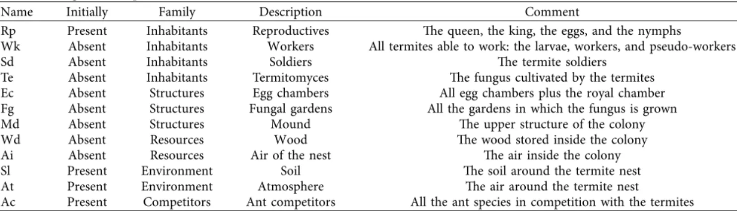
There can be no doubt that ecosystems are complex, despite a few of them remaining simple. Ecosystem pro-cesses are notoriously noisy and difficult to measure, while the biological components of ecosystems often add a strong variance to the overall behavior. Despite this challenge, ecologists need to continue collecting data on ecosystems to improve the understanding of such systems and, ultimately, their management. But where does ecological complexity reside? Is it in the ecosystem state or in the ecosystem dynamics? Ecologists are commonly inclined to scrutinize a snapshot of the ecosystem (the pattern) instead of its long-Table 1: Node categories, names, abbreviations, and descriptions of the termite colony ecosystem modeled using the discrete qualitative model (see Figure 1, adapted from [30]).
Name Initially Family Description Comment
Rp Present Inhabitants Reproductives The queen, the king, the eggs, and the nymphs
Wk Absent Inhabitants Workers All termites able to work: the larvae, workers, and pseudo-workers
Sd Absent Inhabitants Soldiers The termite soldiers
Te Absent Inhabitants Termitomyces The fungus cultivated by the termites
Ec Absent Structures Egg chambers All egg chambers plus the royal chamber
Fg Absent Structures Fungal gardens All the gardens in which the fungus is grown
Md Absent Structures Mound The upper structure of the colony
Wd Absent Resources Wood The wood stored inside the colony
Ai Absent Resources Air of the nest The air inside the colony
Sl Present Environment Soil The soil around the termite nest
At Present Environment Atmosphere The air around the termite nest
Ac Present Competitors Ant competitors All the ant species in competition with the termites
Table 2: List of the rules for modeling termite ecosystem functioning and development.
Rule Comment
(1) Wk+, Te+⟶ Wd−, ai− The workers and the fungi are consuming wood and air
(2) Fg−⟶ Te− The fungi need the fungal gardens in order to survive
(3) Wk+, Sl+⟶ Wd+, Te+, Fg+, Ec+, Md+
The workers are foraging in the soil for wood and fungus; from the soil, the workers are building the fungal gardens, the egg chambers, and the mount
(4) Wd−⟶ Wk−, Te− The workers and the fungus need to eat wood to survive
(5) Rp+, Sl+⟶ Ec+ For the soil, the queen and the king can also build egg rooms
(6) Rp+, Ec+⟶ Wk+ In the egg chambers, the queen and the king are producing eggs that are becoming workers (7) Wk+, Wd+⟶ Sd+, Rp+ Eating wood, the larvae are metamorphosing into soldiers and/or nymphaea (8) Md+, At+⟶ Ai+ The air of the nest is being refreshed by passing through the mound and exchanging with the
atmosphere
(9) Wk−⟶ Fg−, Sd− The soldiers cannot survive without the workers to feed them, and the fungal gardens need maintenance by the workers
(10) Wk−, Rp−⟶ Ec− The egg chambers need maintenance by the workers or the reproductives; otherwise they collapse (11) Sd+⟶ Ac− The soldiers are killing ant competitors intruding into the colony
(12) Ac+, Sd−⟶ Wk−, Rp− Without the soldiers, the ant competitors are invading the colony and killing the workers and the reproductives
(13) Ai−⟶ Rp−, Wk−, Te− The reproductives, the workers, and the fungus need to breathe the air of the nest to survive The conditions of application, realizations, and detailed explanations are given for each rule. The rule arrows indicate the transformation (rewriting) of the network at the next step [30]. Discrete systems are used to exhaustively characterize the dynamics of an integrated ecosystem (Methods in Ecology and Evolution, 00: 1–13 [30]).
term (process) dynamics. For example, it is inappropriate to study traditional ecosystem potential on the basis of isolated states (Figure 6) rather than the trajectories connecting them (Figure 4). Ecosystems are historical objects experiencing abrupt changes with probable nonergodic behaviors [18, 55, 56]. Most ecosystem studies have been performed over relatively short timescales, typically over one or two human generations. We still know very little about the long-term behavior of ecosystems, i.e., over several generations of the slowest component, despite increasing efforts in his-torical ecology and paleoecology (e.g., [69, 70]). The usual variables under long-term study often concern vegetation and climate, but rarely fauna, soils, and/or human com-ponents. An understanding of long-term ecosystem be-haviors is now becoming an imperative, with realistic modeling as a corollary.
At this stage, a decisive recommendation is not to neglect the process of fitting the model to observations. To date, it has been rare for traditional potentials to fit ob-served ecosystems [27, 44] and has mainly involved pattern and fragmented datasets. To our knowledge, it has not once been the case with process and ecosystem dynamics [32]. Most of the time, the model is displayed to interpret a posteriori observations, and not strictly fitted to them. This critical preliminary step should be performed with more variables, on longer trends and with finer models, a comment which is true for discrete event models too. Data collection in ecology is particularly challenging, consid-ering the cost of surveying a complete ecosystem (i.e., most components) and considering the number of components, but substitutes can be found to start this program of work. Some chemostat and controlled experiments may allow for high resolution and long-term measurements [71], while some large scale ecosystems have begun to have rich da-tabases too [27]. There appears to us to be an urgent need to start calibrating potential-like and discrete-event models on such complex data and to test their related hypotheses. To generalize the potential concept to various contrasting ecosystems, it will be necessary to confirm its power and usefulness.
These recommendations may all be summarized as a triangle of improvements that feed into the three main components of any research theme of complexity, namely, data, model, and concept research. In between, there are fits, ideas, and tools that enable continuous testing of emerging concepts such as state spaces and potential surfaces. At present, some sides of this triangle appear to be missing, with further studies being required to produce a satisfying theory of ecosystem. As shown above, potential-like surfaces may not be the most appropriate concepts for describing and understanding complex ecosystem behaviors and dynamics. Even in cases where the potential concept proved appro-priate, it would be fruitful and heuristic to search for some additional views [32]. For example, we recently proposed also looking for linguistic principles in living systems and ecosystems [72].
Simultaneously seeking new mathematical tools is also an imperative; such models include these underused
qual-itative discrete event models [30]. Other tools have been
proposed in the past, and it would be a shame to ignore them or fail to fully acknowledge them. For example, Thom’s work shows rich but unwieldy algebra specifically for potentials in any field [25]. Economic and ethological studies have already tried, unsuccessfully, to use these tools. In addition, we believe it is crucial to develop possibilistic models for ex-haustive characterization of ecosystem trajectories, instead of probabilistic models focusing on a few dominant tra-jectories only.
In conclusion, we would like to warn the ecologist community of the hazards of drawing an analogy between physical and ecological systems. The history of ecology has already shown how this analogy once sent the community down potentially erroneous and/or useless pathways [11]. It is often fruitful to borrow concepts from other scientific fields, but they need to be tailored to the questions under examination at best and, at worst, they could send us off down a slippery, dangerous slope.
Data Availability
No data were used to support this study.
Conflicts of Interest
The authors declare that they have no conflicts of interest.
References
[1] I. A. Hatton, K. S. McCann, J. M. Fryxell et al., “The predator-prey power law: biomass scaling across terrestrial and aquatic biomes,” Science, vol. 349, no. 6252, 2015.
[2] S. K´efi, V. Miele, E. Wieters, S. Navarrete, and E. Berlow, “How structured is the entangled bank? The surprisingly simple organization of multiplex ecological networks leads to increased persistence and resilience,” PLoS Biology, vol. 14, no. 8, Article ID e1002527, 2016.
[3] R. M. May, Stability and Complexity of Model Ecosystems, Princeton University Press, Princeton, NY, USA, 1974. [4] E. Th´ebault and C. Fontaine, “Stability of ecological
communities and the architecture of mutualistic and trophic networks,” Science, vol. 329, no. 5993, pp. 853–856, 2010.
[5] R. C. Dewar, C. H. Lineweaver, R. K. Niven, and K. Regenauer-Lieb, “Beyond the second law,” Entropy
Pro-duction and Non-Equilibrium Systems, Springer, Berlin,
Germany, 2011.
[6] B. C. Patten, “Network integration of ecological extremal principles: exergy, emergy, power, ascendency, and indirect effects,” Ecological Modelling, vol. 79, no. 1–3, pp. 75–84, 1995. [7] E. Ostrom, “A general framework for analyzing sustainability of social-ecological systems,” Science, vol. 325, no. 5939, pp. 419–422, 2009.
[8] I. Steffan-Dewenter, M. Kessler, J. Barkmann et al., “Tradeoffs between income, biodiversity, and ecosystem functioning during tropical rainforest conversion and agroforestry in-tensification,” Proceedings of the National Academy of
Sci-ences, vol. 104, no. 12, pp. 4973–4978, 2007.
[9] C. Gaucherel, “Ecosystem complexity through the lens of logical depth: capturing ecosystem individuality,” Biological
[10] S. P.-V. Frontier, D. A. Lepˆetre, D. Davoult, and C. Luczak,
Ecosyst`emes. Structure, Fonctionnement, Evolution, Dunod,
Paris, France, 4th edition, 2008.
[11] C. Gaucherel, “Physical concepts and ecosystem ecology: a revival?” Journal of Ecosystem and Ecography, vol. 8, 2018. [12] R. E. Ricklefs and G. L. Miller, Ecology, Freeman, New York,
NY, USA, 4th edition, 2000.
[13] R. H. Mac Arthur and E. O. Wilson, The Theory of Insular
Zoogeography, Princeton Univesity Press, Princeton, NY,
USA, 1963.
[14] C. S. Holling, “Resilience and stability of ecological systems,”
Annual Review of Ecology and Systematics, vol. 4, no. 1,
pp. 1–23, 1973.
[15] M. Scheffer, Critical Transitions in Nature and Society, Princeton University Press, Princeton, NJ, USA, 2009. [16] M. Scheffer, S. Carpenter, J. A. Foley, C. Folke, and B. Walker,
“Catastrophic shifts in ecosystems,” Nature, vol. 413, no. 6856, pp. 591–596, 2001.
[17] B. Walker, C. S. Holling, S. R. Carpenter, and A. Kinzig, “Resilience, adaptability and transformability in social-eco-logical systems,” Ecology and Society, vol. 9, no. 2, 2004. [18] C. Gaucherel, H. Th´ero, A. Puiseux, and V. Bonhomme,
“Understand ecosystem regime shifts by modelling ecosystem development using boolean networks,” Ecological Complexity, vol. 31, pp. 104–114, 2017.
[19] R. V. Sol´e and J. Bascompte, Self-Organization in Complex
Ecosystems, Princeton University Press, Princeton, NJ, USA,
2006.
[20] M. Hirota, M. Holmgren, E. H. Van Nes, and M. Scheffer, “Global resilience of tropical forest and savanna to critical transitions,” Science, vol. 334, no. 6053, pp. 232–235, 2011. [21] B. W. Brook, E. C. Ellis, M. P. Perring, A. W. Mackay, and
L. Blomqvist, “Does the terrestrial biosphere have planetary tipping points?” Trends in Ecology & Evolution, vol. 28, no. 7, pp. 396–401, 2013.
[22] C. Gaucherel and V. Moron, “Potential stabilizing points to mitigate tipping point interactions in earth’s climate,”
In-ternational Journal of Climatology, vol. 37, no. 1, pp. 399–408,
2016.
[23] E. H. van Nes, M. Hirota, M. Holmgren, and M. Scheffer, “Tipping points in tropical tree cover: linking theory to data,”
Global Change Biology, vol. 20, no. 3, pp. 1016–1021, 2014.
[24] R. Badii and A. Politi, Complexity, Hierarchical Structures and
Scaling in Physics, Cambridge University Press, Cambridge,
UK, 1997.
[25] R. Thom, Structural Stability and Morphogenesis, Benjamin, Reading, MA, USA, 1975.
[26] F. Accatino, C. De Michele, R. Vezzoli, D. Donzelli, and R. J. Scholes, “Tree-grass co-existence in savanna: interactions of rain and fire,” Journal of Theoretical Biology, vol. 267, no. 2, pp. 235–242, 2010.
[27] M. Scheffer, S. H. Hosper, M.-L. Meijer, B. Moss, and E. Jeppesen, “Alternative equilibria in shallow lakes,” Trends
in Ecology & Evolution, vol. 8, no. 8, pp. 275–279, 1993.
[28] A. C. Staver, S. Archibald, and S. Levin, “Tree cover in sub-Saharan Africa: rainfall and fire constrain forest and savanna as alternative stable states,” Ecology, vol. 92, no. 5, pp. 1063–1072, 2011.
[29] E. H. Van Nes and M. Scheffer, “Slow recovery from per-turbations as a generic indicator of a nearby catastrophic shift,” The American Naturalist, vol. 169, no. 6, pp. 738–747, 2007.
[30] C. Gaucherel and F. Pommereau, “Using discrete systems to exhaustively characterize the dynamics of an integrated
ecosystem,” Methods in Ecology and Evolution, vol. 10, no. 9, pp. 1–13, 2019.
[31] F. Pommereau, Algebras of Coloured Petri Nets, Lambert Academic Publishing (LAP), Riga, Latvia, 2010.
[32] C. H´ely, H. H. Shuggart, B. Swap, and C. Gaucherel, “The drape concept to understand ecosystem dynamics and its tipping points,” 2020.
[33] H. Ehrig, M. Pfender, and H. J. Schneider, “Graph-grammars: an algebraic approach,” in Proceedings of the 14th Annual
Symposium on Switching and Automata Theory (Swat 1973),
pp. 167–180, IEEE Transactions on Cybernetics, Iowa City, IA, USA, October 1973.
[34] J.-L. Giavitto and O. Michel, “Modeling the topological or-ganization of cellular processes,” Biosystems, vol. 70, no. 2, pp. 149–163, 2003.
[35] W. Reisig, Understanding Petri Nets, Springer Berlin Hei-delberg, Berlin, Germany, 2013.
[36] J. S. Turner, The Extended Organism: The Physiology of
Ani-mal-Built Structures, Harvard University Press, Cambridge,
MA, USA, 2009.
[37] M. Cosme, C. H´ely, F. Pommereau et al., “East-African rangeland dynamics: from a knowledge-based model to the possible futures of an integrated social-ecological system. In review,” 2020.
[38] C. Gaucherel, C. Carpentier, I. R. Geijzendorffer, C. Noˆus, and P. F., “Long term development of a realistic and integrated ecosystem,” 2020.
[39] H. G. Fowler, V. Pereira da-Silva, L. C. Forti, and N. B. Saes, “Population dynamics of leaf cutting ants: a brief review,” Fire
Ants and Leaf-Cutting Ants, pp. 123–145, Westview Press,
Boulder, CO, USA, 1986.
[40] M. A. Bl¨atke, M. Heiner, and W. Marwan, “Tutorial,” in Petri
Nets in Systems Biology, Otto-von-Guericke University
Magdeburg, Magdeburg, Germany, 2011.
[41] J.-L. Giavitto, H. Klaudel, and F. Pommereau, “Integrated regulatory networks (IRNs): spatially organized biochemical modules,” Theoretical Computer Science, vol. 431, pp. 219– 234, 2012.
[42] J. M. Dambacher, H. K. Luh, H. W. Li, and P. A. Rossignol, “Qualitative stability and ambiguity in model ecosystems,”
The American Naturalist, vol. 161, no. 6, pp. 876–888, 2003.
[43] B. T. Bestelmeyer, A. Ash, J. R. Brown et al., “State and transition models: theory, applications, and challenges,”
Rangeland Systems, pp. 303–345, Springer, Berlin, Germany,
2017.
[44] M. Scheffer, S. R. Carpenter, V. Dakos, and E. H. van Nes, “Generic indicators of ecological resilience: inferring the chance of a critical transition,” Annual Review of Ecology,
Evolution, and Systematics, vol. 46, no. 1, pp. 145–167, 2015.
[45] B. Berthomieu, P.-O. Ribet, and F. Vernadat, “The tool TINA—construction of abstract state spaces for petri nets and time petri nets,” International Journal of Production Research, vol. 42, 2004.
[46] V. N. Livina, F. Kwasniok, and T. M. Lenton, “Potential analysis reveals changing number of climate states during the last 60 kyr,” Climate of the Past, vol. 6, no. 1, pp. 77–82, 2010. [47] T. M. Lenton, V. N. Livina, V. Dakos, and M. Scheffer, “Climate bifurcation during the last deglaciation?” Climate of
the Past, vol. 8, no. 4, pp. 1127–1139, 2012.
[48] S. H. Strogatz, Nonlinear Dynamics and Chaos: With
Appli-cations to Physics, Biology and Chemistry, Perseus Publishing,
New York, NY, USA, 2001.
[49] J. Lovelock, The Ages of Gaia: A Biography of Our Living Earth, Oxford University Press, Oxford, UK, 2000.
[50] O. Lejeune, M. Tlidi, and P. Couteron, “Localized vegetation patches: a self-organized response to resource scarcity,” Physical
Review E, vol. 66, no. 1, 2002.
[51] C. H. Waddington, “The epigenotype,” Endeavour, vol. 1, pp. 18–20, 1942.
[52] S. Gavrilets, “Highimensional fitness landscapes and speciation,” in Evolution–The Extended Synthesis, M. Pigliucci and G. B. M¨uller, Eds., pp. 45–79, MIT Press Scholarship Online, Cam-bridge, MA, USA, 2010.
[53] H. Ledford, “Language: disputed definitions,” Nature, vol. 455, no. 7216, pp. 1023–1028, 2008.
[54] V. V. Ogryzko, “Erwin schroedinger, francis crick and epigenetic stability,” Biology Direct, vol. 3, no. 1, p. 15, 2008.
[55] J. Vollmer, “Chaos, spatial extension, transport, and non-equi-librium thermodynamics,” Physics Reports, vol. 372, no. 2, pp. 131–267, 2002.
[56] C. Gaucherel, P. H. Gouyon, and J. L. Dessalles, Information, the
Hidden Side of Life, ISTE, Wiley, London, UK, 2019.
[57] E. P. Odum, “Energy flow in ecosystems: a historical review,”
American Zoologist, vol. 8, no. 1, pp. 11–18, 1968.
[58] F. Bouchard, “How ecosystem evolution strengthens the case for functional pluralism,” Functions: Selection and Mechanisms, pp. 83–95, Springer Netherlands, Dordrecht,
Netherlands, 2013.
[59] S. J. Gould, Wonderful Life: The Burgess Shale and the Nature of
History, W. W. Norton & Company, New York, NY, USA, 1989.
[60] C. H´ely, P. Braconnot, J. Watrin, and W. Zheng, “Climate and vegetation: simulating the African humid period,” Comptes
Rendus Geoscience, vol. 341, no. 8-9, pp. 671–688, 2009.
[61] K. Sterelny, “Contingency and history,” Philosophy of Science, vol. 83, pp. 1–18, 2015.
[62] J. Ratnam, W. J. Bond, R. J. Fensham et al., “When is a “forest” a savanna, and why does it matter?” Global Ecology and
Biogeog-raphy, vol. 20, no. 5, pp. 653–660, 2011.
[63] Y. Bergeron and A. Leduc, “Relationships between change in fire frequency and mortality due to spruce budworm outbreak in the southeastern Canadian boreal forest,” Journal of Vegetation
Sci-ence, vol. 9, pp. 493–500, 1998.
[64] B. J. Stocks, M. A. Fosberg, T. J. Lynham et al., “Climate change and forest fire potential in Russian and Canadian boreal forests,”
Climatic Change, vol. 38, no. 1, pp. 1–13, 1998.
[65] A. G. Tansley, “The use and abuse of vegetational concepts and terms,” Ecology, vol. 16, no. 3, pp. 284–307, 1935.
[66] N. Chomsky, Studies on Semantics in Generative Grammar, Mouton & Co., NV Publishers, La Haye, Netherlands, 1972. [67] C. Gaucherel, F. Boudon, T. Houet, M. Castets, and C. Godin,
“Understanding patchy landscape dynamics: towards a landscape language,” PLoS One, vol. 7, no. 9, Article ID e46064, 2012.
[68] C. Godin, “Representing and encoding plant architecture: a re-view,” Annals of Forest Science, vol. 57, no. 5, pp. 413–438, 2000. [69] C. L. Crumley, “Historical ecology: a multidimensionalecological orientation,” in Historical Ecology: Cultural Knowledge and Changing Landscapes, C. L. Crumley, Ed.,pp. 1–16, School of American Research Press, Santa Fe, NM,USA, 1994.
[70] C. H´ely, L. Bremond, S. Alleaume, B. Smith, M. T. Sykes, and J. Guiot, “Sensitivity of African biomes to changes in the pre-cipitation regime,” Global Ecology and Biogeography, vol. 15, no. 3, pp. 258–270, 2006.
[71] M. J. Wade, J. Harmand, B. Benyahia et al., “Perspectives in mathematical modelling for microbial ecology,” Ecological
Modelling, vol. 321, pp. 64–74, 2016.
[72] C. Gaucherel, The Languages of Nature. When Nature Writes


![Figure 6: Examples of various synthetic representations of system dynamics, including a potential-like surface (a) [16], the epigenetic surface (b) [51], and the drape concept (c) inspired from [32]](https://thumb-eu.123doks.com/thumbv2/123doknet/13871155.446238/10.900.96.801.101.929/examples-synthetic-representations-dynamics-including-potential-epigenetic-inspired.webp)