Task 3: Report on Task 3: Extreme Canadian Climates - Northern and Coastal

https://doi.org/10.4224/20378117

READ THESE TERMS AND CONDITIONS CAREFULLY BEFORE USING THIS WEBSITE.

https://nrc-publications.canada.ca/eng/copyright

Vous avez des questions? Nous pouvons vous aider. Pour communiquer directement avec un auteur, consultez la

première page de la revue dans laquelle son article a été publié afin de trouver ses coordonnées. Si vous n’arrivez pas à les repérer, communiquez avec nous à PublicationsArchive-ArchivesPublications@nrc-cnrc.gc.ca.

Questions? Contact the NRC Publications Archive team at

PublicationsArchive-ArchivesPublications@nrc-cnrc.gc.ca. If you wish to email the authors directly, please see the first page of the publication for their contact information.

Archives des publications du CNRC

For the publisher’s version, please access the DOI link below./ Pour consulter la version de l’éditeur, utilisez le lien DOI ci-dessous.

Access and use of this website and the material on it are subject to the Terms and Conditions set forth at

Task 3: Report on Task 3: Extreme Canadian Climates - Northern and

Coastal

Cornick, S. M.

https://publications-cnrc.canada.ca/fra/droits

L’accès à ce site Web et l’utilisation de son contenu sont assujettis aux conditions présentées dans le site LISEZ CES CONDITIONS ATTENTIVEMENT AVANT D’UTILISER CE SITE WEB.

NRC Publications Record / Notice d'Archives des publications de CNRC:

https://nrc-publications.canada.ca/eng/view/object/?id=2c2ae705-ab7b-483c-b939-a77587214c42 https://publications-cnrc.canada.ca/fra/voir/objet/?id=2c2ae705-ab7b-483c-b939-a77587214c42

T a s k 3 : R e p o r t o n T a s k 3 : E x t r e m e C a n a d i a n

C l i m a t e s – N o r t h e r n a n d C o a s t a l

B - 1 2 3 9 . 3

C o r n i c k , S . M .

J u l y 7 , 2 0 0 5

The material in this document is covered by the provisions of the Copyright Act, by Canadian laws, policies, regulations and international agreements. Such provisions serve to identify the information source and, in specific instances, to prohibit reproduction of materials without written permission. For more information visit http://laws.justice.gc.ca/en/showtdm/cs/C-42

Les renseignements dans ce document sont protégés par la Loi sur le droit d'auteur, par les lois, les politiques et les règlements du Canada et des accords internationaux. Ces dispositions permettent d'identifier la source de l'information et, dans certains cas, d'interdire la copie de documents sans permission écrite. Pour obtenir de plus amples renseignements : http://lois.justice.gc.ca/fr/showtdm/cs/C-42

PERD-079 -

Engineered Building Envelope Systems to Accommodate

High Performance Insulation with Outdoor/Indoor Climate Extremes

Task 3

Report on Task 3: Extreme Canadian Climates – Northern and

Coastal

S. M. Cornick

Research Officer

Institute for Research in Council

National Research Council of Canada

Report No: B-1239.3

Report Date: July 7, 2005

Contract No: B-1239

Program: Building

Envelope & Structure

53 pages

This report may not be reproduced in whole or in part without the written consent of both

the client and the National Research Council Canada

This document was created for electronic viewing. Printing this document may result in a

loss in quality from the original document.

Table of Contents

Table of Contents... ii

List of Figures ... iii

List of Tables... iii

List of Charts ... iii

List of Maps... iv

Executive Summary... 1

Objectives and Scope ... 2

Extreme Climates ... 2

General Purpose Climate Classifications... 2

Building Related Climate Classifications ... 3

A Modified Köppen Classification Scheme... 3

A Thornthwaite Scheme ... 3

DOE Proposed Climate Regions ... 5

Extremely Cold Climates... 6

Days with Minimum Temperature Below -20

C ... 9

Relationship between -20 days and HDD18

C ... 9

Recommended Approach for Characterizing Extremely Cold Climates ... 10

Extremely Wet and Humid Climates ... 11

Recommended Approach for Characterizing Extremely Wet and Humid Climates . 15

Suggested Locations... 16 Summary ... 17 References ... 18 Charts ... 19 Maps ... 28 Appendix ... 40

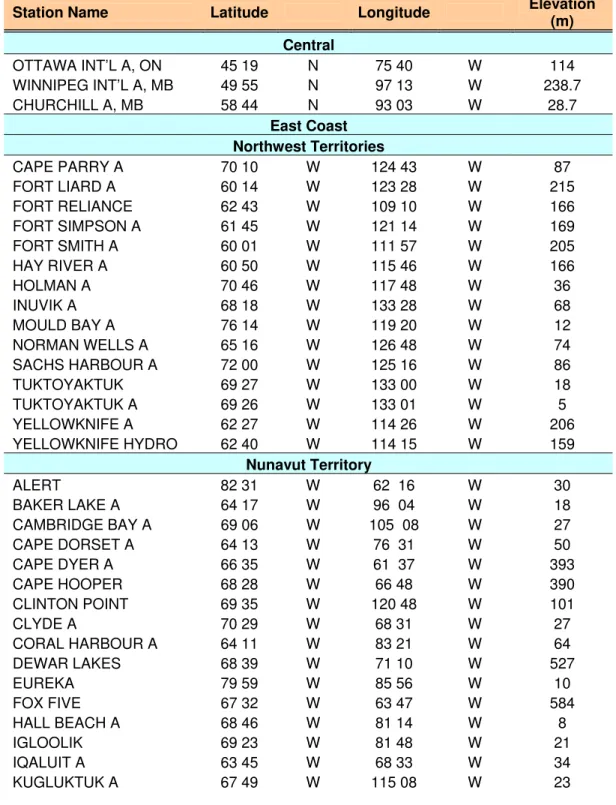
Locations considered in the study... 40

List of Figures

Figure 1 – Variation of number of days with minimum daily temperature below -20 oC and -30 oC with

HDD18 oC. ... 10

Figure 2 – Relationship between mean number of days with minimum daily temperature below -20 oC and HDD18 oC. ... 11

Figure 3 – Correlation between MI and mean annual rainfall for Table C locations in the 1995 NBCC... 15

List of Tables

Table 2 – Definitions of climatic symbols and boundaries for a Thornthwaite scheme ... 5

Table 3 – Definitions of climatic symbols and boundaries for proposed DOE climate zones... 7

Table 4 – Weather parameters for a few selected locations... 9

Table 5 – Table of values relating mean number of days with minimum daily temperature below -20 oC and HDD18 oC ... 12

Table 6 – Weather parameters for recommended locations... 18

Table A.1 – Locations considered in this study for extreme cold... 40

Table A.2 – Locations considered in this study for extreme humidity. ... 42

Table A.3 – Selected climate normal information for Inuvik, NT... 43

Table A.4 – Selected climate normal information for Yellowknife, NT. ... 44

Table A.5 – Selected climate normal information for Iqaluit, NU. ... 45

Table A.6 – Selected climate normal information for Prince Rupert, BC. ... 46

List of Charts

Chart 2 – Bar chart showing mean monthly number of days with minimum below -20 oC and the total days in the month for Iqaluit. ... 20

Chart 3 – Bar chart showing mean monthly number of days with minimum below -20 oC and the total days in the month for Ottawa. ... 21

Chart 4 – Bar chart showing mean monthly number of days with minimum below -20 oC and the total days in the month for Prince Rupert... 22

Chart 5 – Bar chart showing mean monthly number of days with minimum below -20 oC and the total days in the month for Whitehorse. ... 23

Chart 6 – Bar chart showing mean monthly number of days with minimum below -20 oC and the total days in the month for Winnipeg. ... 24

Chart 7 – Bar chart showing mean monthly number of days with minimum below -20 oC and the total days in the month for Yellowknife... 25

Chart 8 – Bar chart showing the mean monthly rainfall for five coastal locations (three west coast and two east coast) and two continental locations. ... 26

Chart 9 – Line plot showing the average relative humidity for five coastal location (three west coast and two east coast) and two continental locations at 06:00 and 15:00 Local Standard Time. ... 27

List of Maps

Map 1 – International Energy Conservation Code (IECC) Climate Zones proposed by DOE from Briggs [7]... 28 Map 2 – Map of western hemisphere climates using a modified Köppen scheme [10]. ... 29 Map 3 – Map of precipitation effectiveness in Canada using Thornthwaite’s scheme from the National

Atlas of Canada 5th edition. http://atlas.gc.ca/site/english/maps/archives/5thedition... 30 Map 4 – Map of thermal efficiency in Canada using Thornthwaite’s scheme from the National Atlas of

Canada 5th edition. http://atlas.gc.ca/site/english/maps/archives/5thedition ... 31 Map 5 – HDD18oC map of Canada from the National Atlas of Canada 5th edition. The map shows the zonal distribution of temperature. http://atlas.gc.ca/site/english/maps/archives/5thedition... 32 Map 6 – Mean number of days with a minimum temperature below -20 oC for locations considered for this

project. ... 33 Map 7 – HDD18oC for locations considered for this project... 34 Map 8 – Mean annual rainfall, mm, for locations listed in Table C of the 1995 National Building Code of

Canada. ... 35 Map 9 – Mean annual mixing ratio deficit, Kg/Kg dry air, for locations listed in Table C of the 1995

National Building Code of Canada. ... 36 Map 10 – Moisture Index values for locations listed in Table C of the 1995 National Building Code of

Canada. ... 37 Map 11 – Annual Driving-Rain Index map of Canada after Boyd [11] ... 38 Map 12 – Population data for northern locations obtained from the 2001 Census... 39

Executive Summary

For extreme cold climates a scheme based on the probability of occurrence of long periods of extremely cold days was developed. An extremely cold day was defined to be a day where the minimum temperature was below -20 °C. The approach recommended approach for characterizing extremely cold Canadian climates is straightforward. One of two commonly available parameters can be used, or both. The parameters are:

1. Mean number of days where daily minimum is less than -20 oC is 100 or more, and/or

2. Mean number of heating degree-days below 18 ºC is 8000 or more.

A location that exceeds either of these thresholds can be considered to be extremely cold.

For extreme wet and humid climates a modification of a precipitation effectiveness index was used, specifically the MEWS Moisture Index (MI). A threshold limit of 1.414 is recommended. However at that limit and beyond the rainfall term use to calculate the MI becomes dominant therefore rainfall has been suggested as a surrogate criteria where MI values are not available. The following criteria are recommended for selecting extremely wet and humid locations.

1. Extreme wet and humid climates as defined in this study shall be locations where the MI value calculated as per the NBCC 2005 exceeds the theoretical limit of √2 i.e 1.414 or,

2. Where the mean annual rainfall exceeds 1250 mm.

Although not part of the climate survey proper some population data was examined for the extreme cold locations. A lower limit of 1000 residents was set to ensure an adequate building stock for the survey portion of this project. It was felt that for coastal regions there would be a sufficient number of locations large enough to provide a large stock of residential buildings.

Based on the criteria set out five locations are recommended for further examination in this project. The five locations are:

1. Inuvik, Northwest Territories – Extreme cold 2. Yellowknife, Northwest Territories – Extreme cold 3. Iqaluit, Nunavut – Extreme cold

4. Prince Rupert, British Columbia – Extreme wet and humid

5. Halifax (Shearwater), Nova Scotia – Extreme wet and humid, if an eastern location is desired. The weather parameters for the recommended locations are shown in the table below:

City # Days Below -20 C HDD18 C Rainfall, mm MI

Inuvik 144.4 9767 117 0.671

Yellowknife 110 8256 156 0.583

Iqaluit 135.2 10117 198 0.864

Prince Rupert 0.14 3966 2469 2.84

Objectives and Scope

The objectivei of this task is to characterize two types of extreme climates in Canada. The two types of climates are:

o extremely cold climates, and

o extremely wet, humid, and cool climates.

The criteria for characterizing the climates are:

o the energy efficiency of the building envelope, specifically walls, and

o the health and safety of the building with respect to the building envelope, specifically walls, and

o the durability and sustainability of the walls.

The focus of the study is low-rise residential construction. A particular aspect of the study will focus on the indoor environmental conditions as it relates to the energy efficiency and health and safety and durability aspects of the buildings; specifically high internal moisture loads. Indoor environmental extremes are considered in Task 1, “Survey of concurrent extreme indoor and outdoor conditions”, of this project. In this report the characteristics of the two climates of interest will be described. As well communities within these regions will be identified as possible sites for field investigations.

Extreme Climates

What are extreme climates? Before describing extreme climates a digression is order. There is no such thing as an extreme climate per se. When considering the combined use of the terms climate and extreme it is generally assumed that the discussion concerns extreme events such as extreme temperature (maximum recorded temperature) or probability of occurrence of an extreme or maximum event such as the maximum 15-minute rainfall that might occur once in ten years (1 in 10). This is not the context within which the term extreme climate is used in this report. The climate characterization is based on long-term climate data, sometimes referred to as climate normal data. The current set of climate normals as defined by the World Meteorological Organization [1] comprises data from the 1971 to 2000; i.e. 30 years of data. The term

extreme in this report will be applied to climates that when compared relative to other climates seem

extreme with respect to the environmental loads imposed on the building envelope.

Climate Classification Schemes

General Purpose Climate Classifications

There are several different schemes for classifying the world's climate, most them possessing genuine merit. Almost all of the schemes of climate classification have subdivisions and boundaries partly based upon temperature and rainfall parameters which are not meaningful in themselves, but have significance in terms of some non-climatic feature such as vegetation, human comfort, mold growth, wood rot, or the like. If one disregards non-climatic phenomena, it is difficult to provide meaningful temperature-rainfall limits of climatic types. The majority of classification schemes, therefore, are of an applied character.

i

From the initial statement of work: “Climate characterization: Define northern and coastal climate extremes (1 in X years) using available weather data (Environment Canada, DND, and other). The objective is to provide data for design and analysis parameters.” For the purposes of this report is it somewhat premature to consider the provision of climate date for design and analysis purposes. The first stage of this task is merely to identify potential locations of interest for field investigations and later analysis and eventually the design of high performance systems for the regions characterized.

One basis for grouping climate schemes is to divide them into genetic and empirical types. In genetic classifications an attempt is made to group climates into the causative factors (e.g. air masses, wind zones) that may be responsible for them. In empirical classifications, origin is discarded as an organizing principle, and observation and experience provide the essential elements for climatic differentiation. The Köppen classification scheme [2] represents a combined genetic-empirical classification which is largely based on

temperature and human habitability. An alterative scheme to Köppen’s was developed by Thornthwaite [3]

and is related to precipitation effectiveness. Köppen and Thornthwaite’s schemes were developed early in the last century. In the last third of the century interest among climate scientists has shifted towards the use of statistical methods for climate classifications. Köppen/Thornthwaite systems have been superseded for the most part in the research literature however they continue to be used in a pedagogical context. A historical perspective, the status, and the future of climate classification are given by Oliver [4]. Both schemes provide insight into the climates of interest for this project.

Building Related Climate Classifications

There are classification systems that are related to buildings. It not is the purpose of this report to review them all. Many of these systems have been described by Cornick [5],[6] and Briggs [7]. The bulk of the systems for North America can be divided into two groups, namely: 1) classifications for energy codes and standards, and 2) other building related classifications. The methods used to derive these schemes vary. Some are arbitrary, some are applied-empiric, while others are numeric, based on cluster analysis or temperature binned data for example. A rigorous approach using cluster analysis, to developing a new a classification for energy codes and buildings is given by Briggs [7] and is the basis for the new DOE map of proposed climate zone [8].

There is an index of climate severity calculated by Environment Canada [9] that combines the extreme values of 18 climate parameters into a rating from 0 to 100. This index however is geared towards human habitability in that the index comprises four major factors, namely: discomfort, psychological state, safety, and mobility, and is not appropriate for our task. For the purposes of this task however a summary of a Köppen, a Thornthwaite scheme, and Briggs’ proposed scheme will be instructive in helping to identify regions of extreme cold and extremely wet and humid climates.

A Modified Köppen Classification Scheme

One the first proposed eponymous climate classification systems is the Köppen classification [2]. The basic criterion in Köppen’s is human habitability. It is also somewhat related to plant growth. A modified scheme is given below. The scheme is temperature based and consequently the climate zones tend to be zonal with latitude, with one notable exception. The exception is the definition of the dry climate which is based on the difference between evaporation and precipitation and this is a flaw in the unity of the whole system. Nevertheless the scheme seems to adequately characterize the world’s climates for most purposes. Three climates in this scheme are of interest to this project. They are the Temperate (D), Boreal (E), and Tundra (F) climates. The definitions of the climate boundaries are given in Table 1.

A Thornthwaite Scheme

The Thornthwaite system [3] developed in the 1930’s is a rational approach to the definition of climatic types that recognizes four aspects of climate: a Moisture Index; the Seasonal Variation of Effective Moisture, an Index of Thermal Efficiency and the Summer Concentration of Thermal Efficiency. To describe the climatic type of any location, the four factors are combined. For example, Ottawa (BB1 B’1 r b’1) is classified as humid, mesothermal with little or no water deficiency and a summer concentration of thermal efficiency between 61.6% and 68%.

Moisture Index. The moisture regions are determined by a moisture index which is defined as lm = lh - la .

The moisture index is based on a humidity index reflecting water surplus and an aridity index reflecting water deficiency. The humidity index is defined as, lh = 100 s/PET, where s is the water surplus and PET is

the potential evapotranspiration. The aridity index is defined as, la = 100 d/PET, where d is the water

Table 1 – Definitions of climatic symbols and boundaries for a Köppen scheme after Trewartha [10]

A (Tropical) = killing frost absent; in marine areas, cold month over 65 oF (18.3 oC),

r (rainy) = 10 to 12 months wet; 0-2 months dry,

w = winter (low-sun period) dry; more than 2 months dry, s = summer (high-sun period) dry; rare in A climates.

B (Dry) = evaporation exceeds precipitation. Boundary, R = 1/2 T - 1/4 PW where R = Rainfall, in., T = temperature oF, PW = % annual rainfall in winter half Desert/steppe boundary is R = (1/2 T - 1/4 PW)/2 or half the amount of the steppe/humid boundary,

W (German Wuste) = desert or arid, S = steppe or semiarid,

h = hot; 8 months or more with average temperature over 50 oF (10 oC),

k (German Kalt) = cold; fewer than 8 months average temperature above 50 oF (10

o

C),

s = summer dry, w = winter dry.

C (Subtropical) = 8 to 12 months over 50 oF (10 oC); coolest month below 65 oF (18.3 oC),

a = hot summer; warmest month over 72 oF (22.2 oC),

b = cool summer; warmest month below 72 oF (22.2 oC))

f = no dry season; difference between driest and wettest month less than required

for s and w; driest month of summer more than 1.2 in. (3 cm),

s = summer dry; at least three times as much rain in winter half year as in summer

half year; driest, summer month less than 1.2 in. (3 cm); annual total less than 35 in. (88.9 cm),

w = winter dry; at least ten times as much rain in summer half year as in summer

half year.

D (Temperate) = 4 to 7 months inclusive over 50 oF (10 oC),

o = oceanic or marine; cold month over 32 oF (0 oC) [to 36 oF (2 oC) in some

locations inland],

c = continental; cold month under 32 oF (0 oC) [to 36 oF (2 oC)],

a = hot summer; warmest month over 72 oF (22.2 oC),

b = cool summer; warmest month below 72 oF (22.2 oC),

f = no dry season; difference between driest and wettest month less than required

for s and w; driest month of summer more than 1.2 in. (3 cm),

s = summer dry; at least three times as much rain in winter half year as in summer

half year; driest summer month less than 1.2 in. (3 cm); annual total less than 35 in. (88.9 cm),

w = winter dry; at least ten times as much rain in summer half year as in summer

half year.

E (Boreal) = 1 to 3 months inclusive over 50 oF (10 oC). F (Polar) = all months below 50 oF (10 oC),

t = tundra; warmest month between 32 oF (0 oC) and 50 oF (10 oC)

i = ice cap; all months below 32 oF (0 oC).

H (Highland) = undifferentiated highland climates. There is no such thing as a highland

type of climate, however; not in the same sense that there is a tropical wet type or

boreal type. Representative temperature and rainfall curves for highland climates do not exist, and only the most flexible generalizations are broadly applicable. One of the most valuable of these generalizations is that highland climates to a

considerable degree are low-temperature variants of lowland climates in similar latitudes.

Seasonal Variation of Effective Moisture. The seasonal variation of effective moisture, which is expressed by means of the aridity index and the humidity index reflecting water, indicates the presence or absence of a dry period in a moist climate or a moist period in a dry climate.

Index of Thermal Efficiency. The thermal efficiency regions are determined by the index of Average Annual Thermal Efficiency which is derived from potential evapotranspiration values. Potential evapotranspiration expresses the average annual amount of moisture which could be evaporated from the soil and transpired by a continuous vegetation cover given no restrictions in the availability of moisture. The index thus combines thermal (heat energy needed for evapotranspiration) and moisture aspects of the climate. It is expressed in the same units as potential evaporation and precipitation.

Summer Concentration of Thermal Efficiency. The summer concentration of thermal efficiency is the percentage of the average annual potential evapotranspiration (thermal efficiency) accumulating in the three summer months. This factor is primarily a function of latitude, continentality, and oceanity. Variations in elevation, aspect, slope, temperature, length of day, and proximity to large bodies of water also significantly influence values. The definitions of the climate boundaries are given in Table 2.

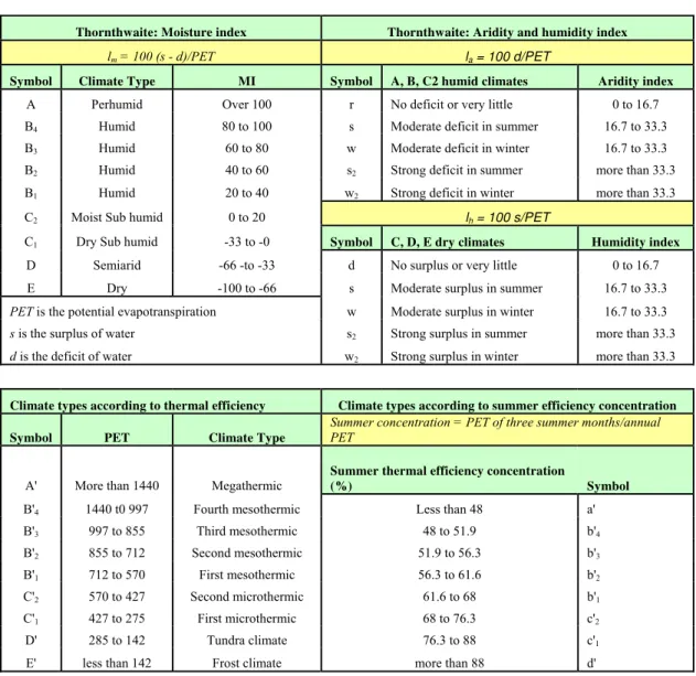
Table 2 – Definitions of climatic symbols and boundaries for a Thornthwaite scheme

Thornthwaite: Moisture index Thornthwaite: Aridity and humidity index

lm = 100 (s - d)/PET la = 100 d/PET

Symbol Climate Type MI Symbol A, B, C2 humid climates Aridity index

A Perhumid Over 100 r No deficit or very little 0 to 16.7 B4 Humid 80 to 100 s Moderate deficit in summer 16.7 to 33.3

B3 Humid 60 to 80 w Moderate deficit in winter 16.7 to 33.3

B2 Humid 40 to 60 s2 Strong deficit in summer more than 33.3

B1 Humid 20 to 40 w2 Strong deficit in winter more than 33.3

C2 Moist Sub humid 0 to 20 lh = 100 s/PET

C1 Dry Sub humid -33 to -0 Symbol C, D, E dry climates Humidity index

D Semiarid -66 -to -33 d No surplus or very little 0 to 16.7 E Dry -100 to -66 s Moderate surplus in summer 16.7 to 33.3

PET is the potential evapotranspiration w Moderate surplus in winter 16.7 to 33.3

s is the surplus of water s2 Strong surplus in summer more than 33.3

d is the deficit of water w2 Strong surplus in winter more than 33.3

Climate types according to thermal efficiency Climate types according to summer efficiency concentration Symbol PET Climate Type

Summer concentration = PET of three summer months/annual PET

A' More than 1440 Megathermic

Summer thermal efficiency concentration

(%) Symbol

B'4 1440 t0 997 Fourth mesothermic Less than 48 a'

B'3 997 to 855 Third mesothermic 48 to 51.9 b'4 B'2 855 to 712 Second mesothermic 51.9 to 56.3 b'3 B'1 712 to 570 First mesothermic 56.3 to 61.6 b'2 C'2 570 to 427 Second microthermic 61.6 to 68 b'1 C'1 427 to 275 First microthermic 68 to 76.3 c'2 D' 285 to 142 Tundra climate 76.3 to 88 c'1

E' less than 142 Frost climate more than 88 d'

DOE Proposed Climate Regions

The proposed DOE climate zoning scheme (from Briggs [7]) was designed for use in energy codes and standards, design guidelines, and building energy analysis. It builds on widely-accepted relationships between climate and energy use. The classification was initially developed using a statistical procedure

called “hierarchical cluster analysis.” This technique uses a distance metric that represents the degree of similarity or dissimilarity between climate sites. Clusters are formed by calculating the distances between all possible pairs in the dataset. The two closest pairs are joined to form a cluster and the centroid of the cluster is calculated. This process is continued until only a single cluster remains. A hierarchical “tree” results comprising progressively nested sub-clusters. By cutting the tree at selected levels results in a group of clusters such that each cluster is relatively homogenous in terms of the clustering variables. However in the end a clean geographically-based set of zones for US was not produced using a comprehensive deterministic clustering technique. Consequently the authors had to rely on more subjective methods to define the final divisions for the proposed DOE climates zones.

In defining the final zones boundaries found in pre-existing classifications that served as a good approximations to the preliminary zones identified by a cluster analysis were used. A humid-dry division based on precipitation effectiveness was used. It was defined in such a way that less precipitation is required to classify a cold climate as humid as for a warm location. The marine division is a variation of various Köppen schemes. Two parameters were chosen for dividing cooling and heating climates, namely CDD10 oC and HDD18 oCii. The classification comprises three main climates; cooling, mixed, and heating climates. The divisions were set subjectively with reference to two previous classification schemes after grouping the locations into humid, dry, and marine zones. The final divisions were then aligned with

political boundaries. Of interest to this project are the sub-artic (8), cold humid (6a), cool humid (5a) and

cool marine (5c) type climates. The distribution o f the DOE climate zones for the continental United

States is shown in Map 1. The definitions of the climate boundaries are given in Table 3

Extremely Cold Climates

Köppen type schemes, like most classifications, do not directly classify the severity of climates. A measure of severity can be inferred if the number of divisions is large but if the number of divisions is too few then the groupings will be too inclusive for the purposes of this project. Returning to the Köppen type classifications, it can be seen that the characteristics of groupings are zonal with latitude, the exception being the Dry (B) type. This of course is a logical result of the basic physics involved. It is of interest here to examine the coldest classifications, namely: Boreal (E) and Polar (F), see Map 2. The distribution of the Polar type climates would seem to justify its use by including most of the far North. The Polar type however excludes many locations that might be considered extremely cold, such as Yellowknife NT, or Churchill MB, when compared to typical locations in the South that are merely cold, such as Edmonton AB. The distribution of the Boreal type, which includes Yellowknife and Churchill, however would seem to be too inclusive.

A Thornthwaite scheme, based on precipitation effectiveness is not appropriate for characterizing climates with respect to temperature. A quick examination of the Canadian climatic regions and thermal efficiency regions makes this clear, see Map 3. However a Thornthwaite scheme based on thermal efficiency seems to produce a map, Map 4, that better differentiates Canadian climates. The result could be bettered however the physical basis for the classification, specifically PET and summer concentration of PET, is not directly related to problem at hand, namely the characterization of extremely cold climates with respect to buildings.

ii

Degree-Days: Degree-days for a given day represent the number of Celsius degrees that the mean temperature is above or below a given base. For example, heating degree-days are the number of degrees below 18º C. If the temperature is equal to or greater than 18, then the number will be zero. Values above or below the base of 18º C are used primarily to estimate the heating and cooling requirements of buildings. Values above 5º C are frequently called growing degree-days, and are used in agriculture as an index of crop growth. Values in the tables represent the average accumulation for a given month or year.

Table 3 – Definitions of climatic symbols and boundaries for proposed DOE climate zones.

Thermal Zone Definitions Climate Zone Representative

City

Thermal Criteria Köppen Class

KöppenDescription 1 - Very hot

a: Humid Miami, FL 5000 < CDD10 o_{C Aw Topical Wet and Dry}

b: Dry N/A 5000 < CDD10 o_{C BWh Tropical Desert}

2 - Hot

a: Humid Houston, TX 3500 < CDD10 o_{C <= 5000 Caf Humid Subtropical (Warm}

summer) b: Dry Phoenix, AZ 3500 < CDD10 oC <= 5000 BWh Arid Subtropical

3 - Warm

a: Humid Memphis, TN 2500 < CDD10 o_{C <= 3500 Caf Humid Subtropical (Warm}

summer) b: Dry El Paso, TX 2500 < CDD10 o_{C <= 3500 BSk/BWh/H Semiarid Middle}

Latitude/Arid Subtropical/Highlands c: Marine San Francisco, CA HDD18 o_{C <= 2000 Cs Dry Summer Subtropical}

(Mediterranean)

4 - Mixed

a: Humid Baltimore, MD CDD10 o_{C <= 2500 and}

HDD18C <= 3000

Caf/Daf Humid Subtropical/Humid Continental (Warm summer) b: Dry Albuquerque, NM CDD10 o_{C <= 2500 and}

HDD18 o_{C <= 3000} BSk/BWh/H Semiarid Middle _{Latitude/Arid}

Subtropical/Highlands c: Marine Salem, OR

(Vancouver BC)

2000 < HDD18 o_{C <= 3000 Cb Marine (Cool Summer)} 5 - Cool

a: Humid Chicago, IL (Toronto ON)

3000 < HDD18 o_{C <= 4000 Daf Humid Continental (Warm}

summer) b: Dry Boise, ID

(Penticton, BC)

3000 < HDD18 o_{C <= 4000 BSk/H Semiarid Middle}

Latitude/Highlands c: Marine (Prince Rupert,

BC)

3000 < HDD18 o_{C <= 4000 Cfb Marine (Cool Summer)} 6 - Cold

a: Humid Burlington, VT; (Ottawa ON)

4000 < HDD18 o_{C <= 5000 Daf/Dfb Humid Continental}

(Warm/Cool summer) b: Dry Helena, MT

(Kamloops, BC)

4000 < HDD18 o_{C <= 5000 BSk/H Semiarid Middle}

Latitude/Highlands

7 - Very Cold Duluth, MN; (Winnipeg, MB)

5000 < HDD18 o_{C <= 7000 Dbf Humid Continental (Cool}

summer)

8 – Sub-artic Fairbanks, AK (Yellowknife, NT)

7000 < HDD18 o_{C Dcf Sub artic}

Adapted from Briggs, Lucas, and Taylor [7]

Major Climate Type Definitions Marine Type Definition

Mean temperature of the coldest month between -3 o_{C and 18} o_{C, and}

Warmest month < 22 o_{C, and}

At least 4 months with mean temperature over 10 oC, and

Dry season in the summer; i.e. rainfall for wettest winter month 3 times driest summer month.

Dry Type Definition

Not Marine, and

Precipitation (cm) < 2 (mean annual temperature + 7 o_C) Humid Type Definition

Not Marine, and

How do the DOE proposed climate zones relate to Canadian locations? Comparing the Briggs and Köppen type schemes it can be seen that both essentially use a thermal criteria, with the Briggs system further refining the thermal zones into sub-groupings of humid, dry, and marine. The division of thermal zones from the stand point of this project seems to correspond well to the subjective criteria defining extremely cold Canadian climates. However, the coldest zone in the DOE grouping includes all locations having greater than 7000 heating degree days below 18oC (classed as sub-artic). This seems to be too inclusive as can be seen by examining the HDD18oC map, see Map 5.

Suppose however we adopt a temperature based approach to defining extremely cold climates focusing on minimum temperatures rather than the monthly average temperatures, used in various Köppen schemes or degree days, used by Briggs. How does this relate to buildings? Recall that this project focuses on three aspects of the envelope performance. These are:

o Energy efficiency –

heat conduction through, convection within, and radiation from the envelope, and

air-leakage, through the envelope either exhilaration or infiltration, and moisture accumulation in the insulation due to air-leakage or vapour diffusion

reducing the effectiveness of the insulation. o Health and safety –

moisture accumulation; mould growth and rot, and

air quality in the interior, windows are likely to be closed for prolonged periods and ventilation equipment may be turned off or not functioning properly, and thermal comfort.

o Durability and sustainability –

damages due to moisture accumulation, and

temperature related damages – movement for example.

A properly designed and constructed envelope should be able to effectively deal with prolonged exposure to cold temperatures. Building codes specify criteria for building design that take exterior temperature into consideration using the 2.5% dry bulb temperature for January. The 2.5% dry bulb temperature is used as the basis for designing and specifying mechanical systems (HVAC), especially the heating system. Certainly the January design temperature could be used as the design temperature for the building envelope. Designing to this temperature means that on average the system, either building envelope or mechanical system, would not perform satisfactorily for 19 hours a year (7.5 for the 1% case), where unsatisfactory performance could mean the occurrence of condensation within the wall, among other things. Could this criterion (or the related 1% January dry bulb temperature) be used as a measure for ranking climates? The answer is a qualified yes. Certainly by setting a threshold limit of say -35 °C for the 2.5% January dry bulb a division could be made amongst cold and extremely cold climates. However this measure does not correlate well with the probability of prolonged periods of extremely cold temperatures. Why should we be interested in prolonged periods of cold? While a lesser design might tolerate short cold snaps a different level of quality is required for periods of extreme cold lasting on the order of three months. Sub-standard designs and constructions will not adequately perform under these conditions. For example, moisture may accumulate in the envelope, inadequate insulation levels may lead to prolonged periods of surface condensation in the interior leading to mould, or energy consumption may higher than expected.

An extremely cold day as defined by Environment Canada is where the minimum temperature for the day is less than -20 °C [9]. How can this be used in defining extreme climates as applied to “Engineered Building Envelope Systems to Accommodate High Performance Insulation with Outdoor/Indoor Climate Extremes?” From the climate normal data there is statistic available that might suit our purposes.

Specifically, the mean numbers of days (per month or year) where the minimum temperature for the day is -20 oC or lessiii.

Days with Minimum Temperature Below -20

C

The objective is to characterize climates that have prolonged periods of extreme cold; i.e. where the minimum for the day < -20 oC. The threshold value for the mean number of days per year will be set, initially at 100 days, a little more than 25% of the year or three months. In locations meeting this criterion there is high probability of extended periods of time occurring where the temperatures are extremely cold without a break. For the three winter months (Dec., Jan., and Feb.) number of days meeting the criteria would exceed 80% of the total.

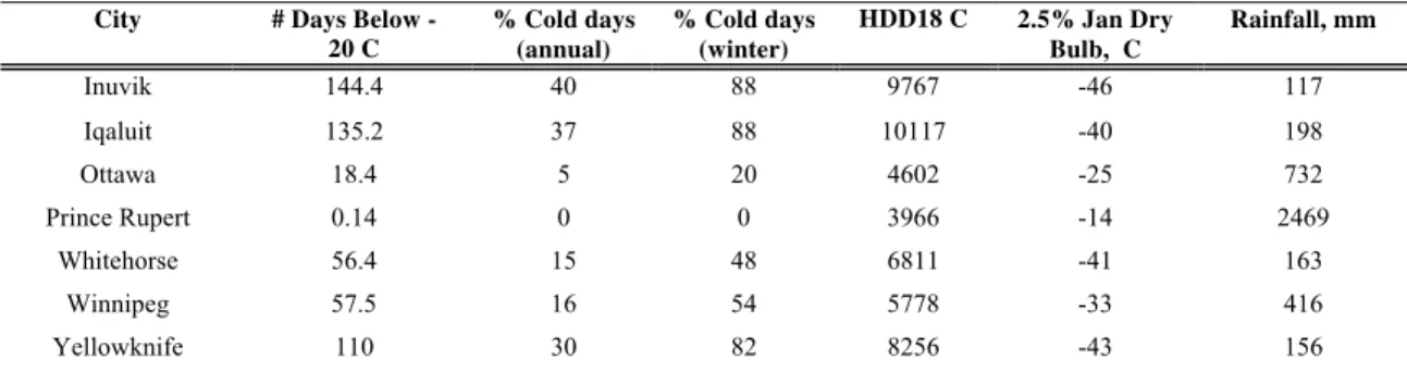
Table 4 lists seven locations. Of the locations listed five would be considered, qualitatively, to be extremely cold locations will the other two would not generally be deemed, from a Canadian perspective, to be extremely cold (Winnipeg and Ottawa). The mean number of days with a minimum below -20 oC and HDD18 oC are given in the table. The monthly distribution of these days throughout the year is shown, Chart 1 to Chart 7 inclusive, for the locations listed. The higher latitude locations clearer exhibit prolonged periods of cold over the winter months. There are however some anomalous spots, Prince Rupert and Whitehorse for example. In fact the entire western mountain range produces temperatures that are anomalously warm given the high latitude of these locations. These anomalies are explained by the presence of mountainous terrain and its effect on the continental weather patterns.

Table 4 – Weather parameters for a few selected locations

City # Days Below -20 C % Cold days (annual) % Cold days (winter) HDD18 C 2.5% Jan Dry Bulb, C Rainfall, mm Inuvik 144.4 40 88 9767 -46 117 Iqaluit 135.2 37 88 10117 -40 198 Ottawa 18.4 5 20 4602 -25 732 Prince Rupert 0.14 0 0 3966 -14 2469 Whitehorse 56.4 15 48 6811 -41 163 Winnipeg 57.5 16 54 5778 -33 416 Yellowknife 110 30 82 8256 -43 156

How was the 100 day threshold selected? Part of the process involved excluding locations that were not deemed to be extremely cold and outside the scope of this project. The mean for Winnipeg is 60 days. Winnipeg is merely cold not extremely cold, although this is a subjective opinion. Whitehorse shows a similar pattern to Winnipeg except that it has more heating degree-days primarily due to the lower temperatures recorded during extremely cold days. Whitehorse is classed as Very Cold (Zone 7) in the DOE climate zoning along with Winnipeg. Map 6 seems to indicate that a threshold of 90 or 100 days seems to qualitatively separate climates that are very cold from extremely cold climates. Therefore, as a preliminary characterization of extreme cold climates for Canada with respect to temperature a threshold value of 100 days is suggested. That is to say that any location where the mean number of days with the minimum temperature for the day is below -20 oC is 100 or greater shall be considered extremely cold and is included in the scope of the project. Table A.1 in the Appendix lists the locations considered so far. These locations are also plotted in Map 6.

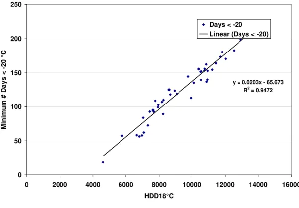
Relationship between -20 days and HDD18

C

If the mean number of days with a minimum temperature less than or equal -20 oC and less than or equal to -30 oC is plotted against HDD18oC, the relationship seems to be linear, see Figure 1. The supposition is that

iii

Number of Days With Specified Parameters gives the average number of days per month or year on which a specific meteorological event occurs.

the greater the mean number of days below a certain threshold the greater the chance of prolonged cold snaps with low temperatures. Ottawa on average has about 19 days during the year with the minimum temperature below -20 oC (1 day below -30 oC) whereas Yellowknife 110 (54 below -30 oC). The number of heating degree-days and the mean days below -20 oC and -30 oC are directly proportional. If one assumes that the risk of unsatisfactory performance increases with the number of days below -20 oC and -30 oC then HDD18oC could be used as a surrogate for that risk. The relationship between HDD18oC and the number of days below -20 oC is shown in Figure 2 and correspondence between heating degree-days and number of days below -20 oC is given in Table 5. The corresponding HDD18oC values for the 90 and 100 day thresholds proposed above are 7700 and 8200 respectively. This suggests that if HDD18oC was to be used as a criterion for establishing extremely cold climates that the threshold value would be 8000 heating degree-days (about 96 days below – 20 oC). Map 7 shows the values of HDD18oC for the locations considered so far.

Recommended Approach for Characterizing Extremely Cold Climates

The approach recommended approach for characterizing extremely cold Canadian climates is straightforward. One of two commonly available parameters can be used, or both. The parameters are:

1. Mean number of days where daily minimum is less than -20 oC is 100 or more, and/or

2. Mean number of heating degree-days below 18 ºC is 8000 or more.

A location that exceeds either of these thresholds can be considered to be extremely cold. The thresholds are based on the assumption that either parameter is a measure of the probability of extremely cold temperatures occurring on a prolonged basis with few breaks in the cold spell. There are several locations that meet the criteria for extreme cold, Yellowknife, Iqaluit or Inuvik for example. Both these locations have a reasonably large population, enough to ensure an adequate stock of buildings for field investigations and are relatively easy to access.

Figure 1 – Variation of number of days with minimum daily temperature below -20 oC and -30 oC with

HDD18 oC. y = 0.0124x - 57.786 R20.9683 = y = 0.0232x - 92.697 R20.9605 = -20 0 20 40 60 80 100 120 140 160 0 2000 4000 6000 8000 10000 12000 HDD18°C Mean Days w ith minimum ... <= -20 °C <= -30 °C

Figure 2 – Relationship between mean number of days with minimum daily temperature below -20 oC and HDD18 oC. y = 0.0203x - 65.673 R2 _{= 0.9472} 0 50 100 150 200 250 0 2000 4000 6000 8000 10000 12000 14000 16000 HDD18°C M ini mu m # D ays < -20 °C Days < -20 Linear (Days < -20)

Extremely Wet and Humid Climates

Extremely wet and humid climates effect buildings in the following ways: o Energy efficiency

Moisture accumulation in the insulation can reduce the insulating effectiveness of certain materials. In wet or humid climates the normal moisture content of the materials will be naturally high, during cooler periods internal moisture loads can further increase the moisture content reducing the energy efficiency of the envelope. Water penetration of the wall cladding can have similar effects. o Health and safety

Climates that have a high relative humidity, expressed as vapour pressure or mixing ratio, tend to have a significant amount of rain and a low drying potential. Moisture accumulation beyond the already high normal moisture contents could potentially lead to mould growth (a health issue) and or rot (a safety issue).

Thermal comfort. o Durability and sustainability

Damages due to moisture accumulation in the envelope can reduce the durability of components leading to shortened service lives and premature failure reducing the overall sustainability of the asset.

The characterization of extremely wet and humid climates is somewhat more difficult than the

Table 5 – Table of values relating mean number of days with minimum daily temperature below -20 oC and HDD18 oC # days = hDD18 m + b m 0.0203 b -65.673 Mean # days below -20 oC HDD18 oC HDD18 oC Mean # days below -20 oC 0 3235.123 0 0 50 5698.177 2500 0 60 6190.788 3000 0 70 6683.399 3500 5.377 80 7176.01 4000 15.527 90 7668.621 4500 25.677 100 8161.232 5000 35.827 110 8653.842 5500 45.977 120 9146.453 6000 56.127 130 9639.064 6500 66.277 140 10131.67 7000 76.427 150 10624.29 7500 86.577 160 11116.9 8000 96.727 170 11609.51 8500 106.877 180 12102.12 9000 117.027 190 12594.73 9500 127.177 200 13087.34 10000 137.327 210 13579.95 10500 147.477 220 14072.56 11000 157.627 230 14565.17 11500 167.777 240 15057.78 12000 177.927 250 15550.39 12500 188.077

Wet and humid climates as defined by Köppen and Briggs

Köppen type classification schemes are essentially based on temperature. The definition of dry versus humid climates in these schemes does not follow the underlying principle of the classification. The boundary between dry and humid climates is based on empirical relationships between the amount of precipitation and temperature. The definition is reproduced below [10]:

B (Dry) = evaporation exceeds precipitation. Boundary, R = 1/2 T - 1/4 PW where R = Rainfall, in., T = temperature oF, PW = % annual rainfall in winter half Desert/steppe boundary is R = (1/2 T - 1/4 PW)/2 or half the amount of the steppe/humid boundary,

W (German Wuste) = desert or arid, S = steppe or semiarid,

h = hot; 8 months or more with average temperature over 50 oF (10 oC),

k (German Kalt) = cold; fewer than 8 months average temperature above 50 oF (10 oC),

s = summer dry, w = winter dry.

All the other divisions in the Köppen scheme are temperature based. Climates are sub-classed according to precipitation indicating whether there have dry or wet seasons. Looking at a map of Köppen based climate

zones for North American it can be seen that the dry climates cut across the other climate zones without regard to temperature, see Map 2. Briggs’ scheme [7] is also thermally based and uses an empirical formula similar to Köppen for dividing humid and dry climates: Precipitation (cm) >= 2 (mean annual temperature + 7 oC).

Briggs’ scheme allows for more refinement in distinguishing between humid and dry climates within the major thermal zones mainly through characterizing climates as humid, dry, or marine based on temperature and a precipitation effectiveness term. Both schemes distinguish marine climates which are of interest to this project. The major criterion for defining marine climates is temperature, although Briggs’ scheme includes a criterion limiting the relative amount of rainfall in the summer and winter months (Köppen is somewhat more flexible in this regard primarily because the classification scheme is global in perspective). Both schemes however do not adequately characterize climates with respect to moisture since both are essentially temperature based, Köppen’s is based plant growth and human habitability and Briggs’ is based on building energy use. Another approach must be considered, although Köppen’s division of humid and dry climates gives a hint as to how to proceed: the boundary for dry climates is where evaporation exceeds

precipitation.

Wet and humid climates as defined by Thornthwaite

Thornthwaite’s scheme is based first and foremost on precipitation and evaporation. The main groupings are based on the ratio of precipitation and evaporation. Sub-classifications deal with the concentration or distribution of the main parameters during the year. The main parameters are: precipitation surplus, precipitation deficit, and potential evapotranspiration. The division between dry and humid climates in this system is where the water surplus equals the deficit. A climate would be classified first according to the precipitation effectiveness, the ratio of surplus or deficit to PET. Subclasses would indicate whether or not there is a dry period in a wet climate or a wet period in a dry climate. The next major classification is thermal efficiency, simply the PET. Subclasses characterize the concentration of drying potential in the summer months. Maps of Canada characterized using Thornthwaite system are shown in Map 3 and Map 4. Can this scheme be made use of this study? The answer is perhaps.

For this project perhumid climates, type A, are of interest. In Canada there a several regions of this type (see Map 3). The main regions are, not unexpectedly, on the east and west coasts. Ideally an r type subclass is desirable; that is a humid climate without a significant dry period. All the A type climates in Canada are classed as type r. The next major Thornthwaite index is thermal efficiency, or potential evapotranspiration,

PET. Since PET implicitly incorporates temperature there is a limit to the values of PET in Canada,

specifically, B’1 the first mesothermic. Not surprisingly most of these climates occur in warmer regions in the country, coloured in red in Map 4. For the purposes of this project a climate with the least amount PET would be of greatest interest, however the areas with the least PET also tend to be the coldest and driest according to the precipitation effectiveness measure. The perhumid climates with the least amount of PET are located on the east coast. This would seem to suggest that perhaps the climates on the east coast are more severe or extreme than those on the west coast. Most of the climates under consideration here are classed, in terms of summer concentration of thermal efficiency, b’2 or less. That is to say the amount of

PET is spread out throughout the year, around 60% summer concentration for b’2 and declining to 50% to

for a b’4 classed climate. The remainder of the PET is spread out over the remaining 9 months of the year. A higher summer concentration of thermal efficiency is typical of colder climates.

There are a few difficulties in using a Thornthwaite scheme for determining what might constitute an extreme wet and humid climate for buildings. First, the concept of a surplus or a deficit is related to the water requirements for plant growth. This is not correct for buildings. Any precipitation, specifically rainfall, should be considered as a surplus for building related issues. Correspondingly with respect to buildings there are no deficits. Second, precipitation includes both frozen and liquid water. Most moisture related problems in buildings are related to rainfall and not snow. Consequently for the purposes of investigating building related problems the Thornthwaite scheme described may overestimate the precipitation effectiveness of some regions, such as the east coast where significant amounts of snow are included in the precipitation amounts. Third, PET is also related to vegetation – in the case of buildings PE

(Potential Evaporation) should be used. Finally, the divisions of the scheme seem to be too broad to distinguish between extreme and non-extreme wet and humid climates.

The MEWS Moisture Index (MI) Approach

A modification of the Thornthwaite precipitation effectiveness approach was developed for the MEWS project [5]. The first change was made to the lm term. Mean annual rainfall was substituted for the

difference between the humidity index, lh and aridity index, la. See Map 8 for the mean annual rainfall

values for all the locations in Table C of the 1995 National Building Code of Canada. Instead of using PET an estimate the PE derived from the mean saturation mixing ratio deficit was used. See Map 9 for the values of this estimate of PE for all the Table C locations. The rainfall and mixing ratio deficit portions of the index are normalized and the value of the index is calculated as the root of the sum of the squares rather than the simply ratio used by Thornthwaite. The result of this is shown in Map 10. The map corresponds rather well with Thornthwaite’s precipitation effectiveness scheme … as it should.

There are a few issues with the MI approach as currently applied. First, the selection of the values to normalize the terms comprising the MI is not well established. Zero is an appropriate value for both evaporation and rainfall but what about the selection of the maximum values? The maximum average annual rainfall is approximately 11.7 m (Kauai, Hawaii) while the maximum value for Canada is approximately 6.7 m (Henderson Lake, BC). The maximum drying potential is limited by temperature, assuming that relative humidity is 0%. Worldwide the hottest location is in Ethiopia, having a mean annual temperature of 35 oC. Using these values for normalizing the MI terms yields a map where most Canadian climates are indistinguishable. This is a difficultly with the normalization approach. The normalizing values used in producing Map 10 where, 1000 mm for rainfall, and 14.9 Kg/Kg dry air- year (Lytton, BC). The rationale for selecting these was based on, 1) the desire to exclude and include various locations in the MI >= 1 grouping, and 2) a subjective judgment on the correspondence of the resulting map with other maps (Thornthwaite see Map 3, Köppen see Map 2, Boyd [11] see Map 11).

The basis for the MI thresholds is also not well established The Mews approach was defined to give a threshold of 1.0 with a maximum value of √2. The rationale was that MI = 1 represents a location with either the maximum wetting potential or a minimum drying potential (the drying index or PE) and this was the limiting case. Climates having a value of MI of less than one would trend to more drying and present a lesser risk of moisture related damage whereas climates with a MI value greater than one would trend to more wetting and a greater risk. Since for rainfall the normalizing factor chosen was less than the maximum observed there are locations that have MI values greater than the theoretical maximum. As well the other the threshold values were chosen in subjective fashion, increasing or decreasing the thresholds in order to produce a map that corresponds well with existing climate schemes and experience with systemic moisture related failures in the field. See Map 10.

There are other drawbacks of the MI approach, incompatible units for example, and these are outlined in Cornick [5]. However despite the criticisms leveled at this approach the division of climates using this method seems workable and the characterization seems to correspond well with other schemes and field data and experience. A reasonable approach to distinguishing extreme climates is to characterize all climates that exceed the theoretical limit of MI (1.414) as extreme. These are the locations indicated with blue or black dots on Map 10.

Chart 8 plots the mean monthly rainfall for several coastal locations, three on the west coast (Tofino, Prince Rupert, and Vancouver, BC) and two on the east coast (St John’s NF, Halifax, NS) as well as two continental locations (Ottawa, ON and Yellowknife, NT). The west coast rainfall pattern is clearly distinct, comprising winter months with heavy rainfall and a drier summer. By contrast the east coast climates tend to have the rainfall distributed relatively evenly throughout the year. The two continental locations are typical of the class with most of the rain falling in the summer months. Note the large difference in quantity and pattern of rainfall between the coastal and continental locations. Chart 9 plots the average monthly relative humidity, AM and PM, for the same locations. The coastal locations follow the same general pattern and are grouped together with respect to magnitude. The pattern and magnitude of the continental locations is distinctly different from coastal locations. With respect to distinguishing extreme wet and

humid climates among coastal climates relative humidity is not good distinguishing characteristic. Annual rainfall appears to be a better parameter for characterizing extreme wet and humid climates. Notice in Chart 8 how Tofino and Prince Rupert stand out conspicuously from the other coastal locations. It can be seen from Figure 3 that MI is strongly correlated to rainfall. In fact at MI values at and above the theoretical limit the rainfall term is the dominant term in calculating the value of MI. So a simple correlation of MI to rainfall might suffice to distinguish extreme wet and humid climates. The rainfall at which the theoretical limit MI is exceeded is approximately 1250 mm per yeariv.

Figure 3 – Correlation between MI and mean annual rainfall for Table C locations in the 1995 NBCC.

y = 1022.4x - 193.93 R2 = 0.8884 0 500 1000 1500 2000 2500 3000 3500 4000 4500 0 0.5 1 1.5 2 2.5 3 3.5 4 4.5 Moisture Index M e a n an nua l r a inf a ll, mm

Recommended Approach for Characterizing Extremely Wet and Humid Climates

The schemes reviewed so far do not distinguish sufficiently between wet and humid climates to be able to label some as extreme others as not extreme on a quantitative basis. In fact quoting from [9] Canada is a climate of moderate extremesv. Halifax, Saint John, Victoria, and Vancouver hardly seem to qualify as extreme climates. However, that being said in an attempt to use quantitative criteria it is suggested that the following criteria be used for selecting extremely wet and humid locations.

1. Extreme wet and humid climates as defined in this study shall be locations where the MI value calculated as per the NBCC 2005 exceeds the theoretical limit of √2 i.e 1.414 or,

2. Where the mean annual rainfall exceeds 1250 mm.

iv

It is felt that the M >= 1.41 and/or Rainfall > 1250 criteria might be too low. Many of the locations in this grouping are classified as extreme with some hesitation. Further research is required in this area to further refine the criteria. For the purposes of this project at this stage however the criteria will serve.

v

An example of a location that meets the criterion for wet and humid climates is Prince Rupert, BC. Other locations meeting the criterion are listed in Table A.3 in the Appendix.

Population Data of Locations of Interest

Although strictly not a part of the climate characterization, while the climate data was being collected for the preliminary phase of this project, some population data was collected. This was not a comprehensive survey but was mainly concentrated on the northern locations used for characterizing extreme cold climates. It was felt that although the selection of locations for the interior conditions survey and the energy simulation portions of the project (Task 6-A) would be based on climate data population data would also effect the selection, especially with regard to the interior conditions survey. The population was taken from the 2001 census and obtained from the following URL:

http://www12.statcan.ca/english/census01/home/index.cfm

The main criteria for selecting a location were population and accessibility. The population of the location should be a least 1,000 to ensure an adequate selection among the housing stock. The location should also be easily accessible; i.e. ideally should have an airport and be accessible all year round. The population of the northern locations surveyed is shown in Map 12. It is felt that the coastal regions identified will provide a sufficient number of communities that would meet the population and accessibility criteria. From the map certain locations suggest themselves. For cold regions they are Dawson and Whitehorse in the Yukon, Inuvik and Yellowknife in the Northwest Territories, and Iqaluit and Rankin Inlet in Nunavut. A good choice for an extreme coastal location is Prince Rupert BC.

Suggested Locations

The section contains some recommendations for locations to be used for the interior conditions survey (Task 1), the energy simulations (Task 6-A), and the hygrothermal modeling task (Task 5-A). A final criterion for determining the preferences was the ready availability of climate data, specifically the existence of CWEEDS (Canadian Weather Energy and Engineering Data Sets) files and CWEC (Canadian Weather for Energy Calculations) files. Locations marked with an asterisk indicate the preferred locations. Climate normal data are provided in the Appendix for the preferred locations.

Cold region locations:

1. Inuvik NT*. – meets the extreme criteria and population criteria, CWEEDSvi tape exists, CWECvii year exists. See Table A.4 for a summary of long-term climate data.

2. Yellowknife NT*. – meets the extreme criteria and population criteria, CWEEDS tape exists, CWEC year exists. See Table A.5 for a summary of long-term climate data.

3. Iqaluit* – meets the extreme criteria and population criteria, CWEEDS tape exists, CWEC year does not exist.. See Table A.6 – Selected climate normal information for Iqaluit, NU.for a summary of long-term climate data.

4. Rankin Inlet NU. – meets the extreme criteria and population criteria, CWEEDS tape does not exist, CWEC year does not exist.

5. Dawson YK. – meets the extreme criteria and population criteria, CWEEDS tape does not exist, CWEC year does not exist.

6. Whitehorse YK. – does not meet the extreme criteria, meets the population criteria, CWEEDS tape exists, CWEC year exists.

Coastal Locations:

1. Prince Rupert BC*. – meets all the criteria, CWEEDS and CWEC files exist. See Table A.7 for a summary of long-term climate data.

vi

CWEEDS files are used for hygrothermal modeling.

vii

2. Halifax (Shearwater) NS. – meets all the criteria, CWEEDS and CWEC files exist.

Summary

Several generalized climate classification schemes have been reviewed, the focus of the review being the characterizing of extreme cold and extreme wet and humid climates. Two generalized schemes, Köppen’s and Thornthwaite’s were reviewed along with a scheme developed by Briggs for DOE. It was found that temperature-based schemes, Köppen and Briggs, although they adequately characterize Canadian climate, are not adequate for distinguishing extreme climates. Nor was Thornthwaite’s classification, based on precipitation effectiveness, adequate for characterizing extreme wet and humid climates. To be fair however none of these schemes were designed with our current objectives in mind.

For extreme cold climates a scheme based on the probability of occurrence of long periods of extremely cold days was developed. An extremely cold day was defined to be a day where the minimum temperature was below -20 °C. The approach recommended for characterizing extremely cold Canadian climates is straightforward. One of two commonly available parameters can be used, or both. The parameters are:

1. Mean number of days where daily minimum is less than -20 oC is 100 or more, and

2. Mean number of heating degree-days below 18 ºC is 8000 or more.

A location that exceeds either of these thresholds can be considered to be extremely cold.

For extreme wet and humid climates a modification of Thornthwaite’s precipitation effectiveness index was used, specifically the MEWS Moisture Index (MI). Extreme climates were defined as those climates where the value of MI exceeds the theoretical limit. However at or beyond the theoretical limit the rainfall term use to calculate the MI becomes dominant and therefore rainfall has been suggested as a surrogate criteria where MI values are not available. It is suggested that the following criteria be used for selecting extremely wet and humid locations.

1. Extreme wet and humid climates as defined in this study shall be locations where the MI value calculated as per the NBCC 2005 exceeds the theoretical limit of √2 i.e 1.414 or,

2. Where the mean annual rainfall exceeds 1250 mm.

Note that it is felt that the M >= 1.41 and/or Rainfall > 1250 criteria might be too low. Many of the locations in this grouping are classified as extreme with some hesitation. Further research is required in this area to further refine the criteria. For the purposes of this project at this stage however the criteria will serve.

Although not part of the climate survey proper some population data were examined for the extreme cold locations. A lower limit of 1000 residents was set to ensure an adequate building stock for the survey portion of this project. It was felt that for coastal regions there would be a sufficient number of locations large enough to provide a large stock of residential buildings.

Based on the criteria set out five locations are recommended for further examination in this project. This of course does not preclude others from be added. The five locations are:

1. Inuvik, Northwest Territories – Extreme cold 2. Yellowknife, Northwest Territories – Extreme cold 3. Iqaluit, Nunavut – Extreme cold

4. Prince Rupert, British Columbia – Extreme wet and humid

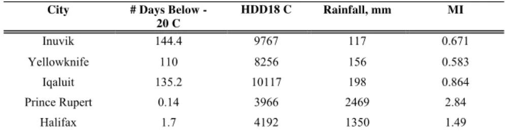
5. Halifax (Shearwater), Nova Scotia – Extreme wet and humid, if an eastern location is desired. The weather parameters for the recommended locations are given in Table 6

Table 6 – Weather parameters for recommended locations

City # Days Below -20 C HDD18 C Rainfall, mm MI Inuvik 144.4 9767 117 0.671 Yellowknife 110 8256 156 0.583 Iqaluit 135.2 10117 198 0.864 Prince Rupert 0.14 3966 2469 2.84 Halifax 1.7 4192 1350 1.49 References

[1] World Climate Data Program: Calculation of Monthly and Annual 30-year Standard Normals, WCDP-No. 10, WMO-TD/WCDP-No. 341, Prepared by a meeting of experts, Washington, D.C., U.S.A., March, 1989.

[2] Köppen, W. Klassification der Klimate nach Temperatur, Niederschlag und Jahreslauf. Petermanns Mitt., Vol. 64, pp. 193-203, 1918.

[3] Thornthwaite, C. W. “The climates of North America according to a new classification. Geog. Rev., Vol. 21, pp. 633-655, 1931.

[4] Oliver, J. “The History, Status, and Future of Climatic Classification.” Physical Geography, Vol. 12,

No. 3, pp. 231-251, 1991.

[5] Cornick, S.M.; Dalgliesh, W.A.; Said, M.N.; Djebbar, R.; Tariku, F.; Kumaran, M.K. Report from Task

4 of MEWS Project - Task 4-Environmental Conditions Final Report, Research Report,

Institute for Research in Construction, National Research Council Canada, 113, pp. 110, October 01, 2002 (RR-113) URL: http://irc.nrc-cnrc.gc.ca/fulltext/rr113/

[6] Cornick, S.M.; Chown, G.A.; Dalgliesh, W.A.; Djebbar, R.; Lacasse, M.A.; Nofal, M.; Said, M.N.; Swinton, M.C.; Tariku, F. Defining Climate Regions as a Basis for Specifying

Requirements for Precipitation Protection for Walls, Ottawa : Canadian Commission on

Building and Fire Codes, National Research Council of Canada, pp. 36, April 12, 2001 (NRCC-45001) URL: http://irc.nrc-cnrc.gc.ca/fulltext/nrcc45001/

[7] Briggs, R. S., R. G. Lucas, Z. T. Taylor, "Climate Classification for Building Energy Code Standards", Parts 1 and 2 2003 ASHRAE Winter Meeting, Papers 4610 and 4611

[8] US Department of Energy – Climate Zone Map, URL:

http://www.energycodes.gov/implement/pdfs/color_map_climate_zones_Mar03.pdf

[9] Phillips, D., The Climates of Canada, Canadian Government Publishing Center, Supply and Services Canada, Catalogue No. En56-1/1990E, Ottawa, 1990.

[10] Trewartha, G. T., An Introduction to Climate, 4th Edition, McGraw-Hill, New York, 1968.

[11] Boyd, D.W. “Driving-Rain Map of Canada”, Technical Note, National Research Council of Canada, Division of Building Research, 398, pp. 3, May 01, 1963 (TN-398)

Charts

Chart 1 – Bar chart showing mean monthly number of days with minimum below -20 oC and the total days

Chart 2 – Bar chart showing mean monthly number of days with minimum below -20 oC and the total days in the month for Iqaluit.

Chart 3 – Bar chart showing mean monthly number of days with minimum below -20 oC and the total days in the month for Ottawa.

Chart 4 – Bar chart showing mean monthly number of days with minimum below -20 oC and the total days in the month for Prince Rupert.

Chart 5 – Bar chart showing mean monthly number of days with minimum below -20 oC and the total days in the month for Whitehorse.

Chart 6 – Bar chart showing mean monthly number of days with minimum below -20 oC and the total days in the month for Winnipeg.

Chart 7 – Bar chart showing mean monthly number of days with minimum below -20 oC and the total days in the month for Yellowknife.

0

50

100

150

200

250

300

350

400

450

500

Jan

Feb

Mar

Apr

May

Jun

Jul

Aug

Sep

Oct

Nov

Dec

M

e

a

n

monthly

r

a

infa

ll

, m

m