Beta and Size Revisited: Evidence from the French Stock Market
Bing Xiao11 Management Science, Université d’Auvergne, Auvergne, France
Correspondence: Bing Xiao, PhD in Management Science, Université d’Auvergne, CRCGM EA 38 49 Université d’Auvergne, Auvergne, France.
Received: July 10, 2016 Accepted: August 4, 2016 Online Published: October 8, 2016 doi:10.5430/ijfr.v7n5p42 URL: http://dx.doi.org/10.5430/ijfr.v7n5p42
Abstract
According to the size effect, small cap securities generally generate greater returns than those of large cap securities. Our study confirms that the size effect does exist in the French stock market, but the difference cannot be explained by the beta levels. It is important to recognize the sign of the excess market return when testing the beta-return relationship. A test of the beta return relationship on the sign of the excess market return finds a significant relationship between conditional beta and returns. However, it seems that the conditional beta does not explain the size effect.
Keywords: conditional beta, market risk premium, ARCH models 1. Introduction
At the beginning of the 1980s, a phenomenon known as the size effect was observed. This size effect noted that small cap securities generate, on average, a greater risk adjusted return than large caps. Banz (1981) and Reinganum (1981) were the first researchers to study the influence of market capitalisation on security returns. They demonstrated that small cap securities generated greater returns than those of large capitalisation and attributed this overperformance of small caps to the remuneration of an additional risk factor. In France, this effect was observed by Hamon and Jacquillat (1992), however, according to them, the size effect would not be observable outside of the year-end transition period.
Both the professional and the academic sectors of the market are interested in the size effect. Two major reasons drive this interest. The first reason is theoretical: if it were possible to show that investment strategy based on small companies is capable of systematically beating the market, the efficient market theory would be faulty. The second reason is more practical: if there are small caps securities with greater performances on average than those of the indices, it would clearly be of interest to investors to identify them.
The size effect also poses a problem with regards to the validity of the Capital Asset Pricing Model (CAPM), validity according to which the expected yield of securities depends on the systematic risk level (the Beta). According to behavioural finance researchers, size effect is proof of the irrationality of individuals. On the contrary, there are researchers who support the concept of rationality which suggests that size effect can be attributed to risk factors other than the market. The robustness of the size effect and the absence of a relation between beta and average return are so contrary to the CAPM that the consensus is that the static CAPM is unable to explain the cross-section of average returns on stocks (see Fama and French, 1992).
In this paper we will examine the French stock market over the period of January 2005 to March 2016 and observe the role of beta in explaining equity returns. The author adopts the dynamic conditional beta approach proposed by Morelli (2011). A univariate GARCH model is used to estimate the dynamic of the volatility of error terms, and a dynamic of the dependence structure between the innovations. The author uses the ratio of the conditional covariance between the residuals from an autoregressive model for each index return and market return to estimate the beta. For the market return, the conditional variance of the residuals from an autoregressive model is used. Modeling the covariance component and the variance component of beta as an ARCH/GARCH process allows for the incorporation of conditional information into the model (see Morelli 2011).
The most commun definitions of small-, large- and mid-cap stocks in France are probably those used by the CAC Index. To be included in the CAC 40, the large-cap, a company must have a market cap of at least 1 billion euros. In regards to the small-cap, Euronext France offers the CAC Small. To be included, a company must have a market cap of $150
million euros on average. And in the middle is the CAC Mid 60. Companies in this index must have a market cap of 150 million euros to 1 billion euros.
The rest of the paper is organized as follows. Section 2 details the reviews of literature. Section 3 presents the methodology and the data. Section 4 discusses our estimates of conditional beta. Section 5 concludes the paper.
2. Literature Review
Financial managers use the Sharpe-Lintner-Black Capital Asset Pricing Model (CAPM) a capital asset pricing model for assessing risk. According to the CAPM, risk is measured by the beta, and there is a linear relationship between the expected return and beta. In many studies a risk-return relationship has not been found. Currently it is agreed upon that the difference in terms of beta levels is not enough to entirely explain the difference in return between small and large caps.
Fama and French (1992, 1993) proposed incorporating additional risk factors into the CAPM to account for the size effect, as the beta was no longer the sole source of risk. Fama and French suggested that the risk in these equities for shareholders was offset by the higher than expected returns of value stocks and small caps. In fact, value stocks and small caps are susceptible to being financially weakened in the event of an economic crisis.
Using the three factor model would both improve the understanding of the observed returns and the size effect. However, interpretation of the two factors that were added to CAPM is not yet accepted. Furthermore, there are other alternatives to CAPM such as the Arbitrage Pricing Theory (ATP) proposed by Ross (1976) and economic type multi-factor models. Even though the size effect creates some difficulties, the CAPM is still a particularly highly regarded reference model and portfolio management tool due to its simplicity.
Based on expectation, the CAPM model is tested using realized returns with assumption that these returns represent and therefore proxy for the excepted returns. The positive relationship between beta and the expected returns is evidence that implies that the excepted return on the market must always be greater than the risk-free rate and there must be a positive expected market risk premium (see Morelli 2011). Using realized data, the realized market risk premium may be negative (see Pettengill et al. 1995).
According to Pettengill et al. (1995), the return on the market will sometimes be less than the risk-free rate. If it was not so, no rational investor would ever invest in risk-free assets. They presume that there is a positive relationship between beta and returns when the realized return on the market is greater than exceeds the risk-free rate (up markets). In down markets, when the realized market return is negative the beta return relationship should be negative as well. Morelli (2011) confirmed this assumption by examining the role of beta in explaining security returns in the UK stock market.
The CAPM is a model based on a hypothetical model-economy. One of the hypothetical conditions assumes the behavior of investor as if they live for only one period. But this assumption is unrelatable as in the real world investors live for many periods. This model also assumes that the betas of the assets remain constant over time. Jagannathan and Wang (1996) suggested that the relative risk of a firm’s cash flow fluctuates over the economic cycles. The financial leverage of firms changed during the expansion and recession. In studies of the American market, a cyclical nature has been revealed in the size effect. Some of these studies have even claimed the disappearance of this anomaly.
According to Reinganum (1999), the size effect could be predicted and large companies outperformed small companies during periods of unfavourable economic conditions. For Dijk (2011), the phenomenon had been cyclic in the period between 1927 and 2005. Similarly, Horowitz, Loughran and Savon (2000) observed that the size effect had disappeared during the period encompassing 1981 to 1997. Schwert (2003) also observed this disappearance of the size effect between 1982 and 2002.
Kim and Burnie (2002) drove the hypothesis according to which size effect might be driven by the economic cycle. L'Her, Masmoudi and Suret (2002) also pointed out that risk premiums vary according to economic conditions. Generally speaking, small caps are penalised to a greater extent during times of crisis due to debt and credit problems, and profit more from times of recovery due to their small structure. Therefore, betas and expected returns are dependant on the nature of the information available at any given point in time and vary over time. These observations led the author to investigate recent developments in the size effect in France.
3. Data and Methodology
3.1 Data
The sample consists of the CAC 40, CAC MID 60 and CAC SMALL index over the period January 21, 2005 to March 11, 2016, a total of 2,852 observations. The one-month T-bill rate is used to proxy for the free-risk rate which
is converted into daily equivalent so as to have a similar frequency with the index returns. The SBF 120 index is used to proxy for the market portfolio. The data required is the returns on the CAC index return series. In order to calculate these returns, the author uses data on the daily price. The requisite data is obtained from the Factset database. The price taken as the daily price is the last trading price of the day.
The summary statistics for the CAC 40, CAC Mid 60 and CAC Small index (Table A1 in the Appendix) reveals a positive skewness, and a negative kurtosis. The CAC index are non-normal at the confidence interval of 99%. So, it is mandated to convert the CAC index series into the return series.
The movements of the stock indices series are non-stationary and cannot be used in this study. Therefore, it is necessary to convert the daily price into the return series. The series of the Russell index are transformed into returns by using the following equation:
= − 1 (1) Where,
= the rate of return at time t = the price at time t
= the price just prior to the time t
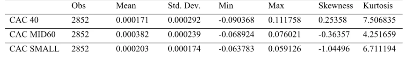
Table 1 summarizes the statistics on returns, showing that the CAC 40 index have an average daily return of 0.000171 and a standard deviation of 0.000292. The skewness coefficient is 0.25358, its sign being common to most financial time series.
The kurtosis value is higher than 3, this indicates the non normal distribution. To account for these characteristics of the date the ARCH family of models should be used. It is imperative when modeling such a series that it be stationary and the data mean-reverting. For this purpose, the Dickey-Fuller test is applied to the returns series (Table A2 in the Appendix), and the results show that the series is stationary. On application, the Phillips-Perron test also indicates that the series is stationary and can be used for modeling purposes (Table A3 in the Appendix).
Table 1. Summary statistics for returns
Obs Mean Std. Dev. Min Max Skewness Kurtosis
CAC 40 2852 0.000171 0.000292 -0.090368 0.111758 0.25358 7.506835
CAC MID60 2852 0.000382 0.000239 -0.068924 0.076021 -0.36357 4.251659
CAC SMALL 2852 0.000203 0.000174 -0.063783 0.059126 -1.04496 6.711194
To confirm whether the return series is stationary or nonstationary both the ADF test and the PP test are used. The values of the ADF test statistic, -52.1122, is less than its test critical value, -1.95, at 5%, level of significance which implies that the CAC 40 return series is stationary. The values of the PP test statistic is less than its test critical value which confirms that the return series is stationary.
The plotted autocorrelation and partial autocorrelation of squared returns indicate dependence which implies time-varying volatility. We can observe this in Figures A1 and A2 in the Appendix which suggests that the series are time-dependent.
3.2 Specification of the Models Used in This Study 3.2.1 ARCH(q) Model and GARCH(p, q) Model
Autoregressive conditional heteroskedasticity (ARCH) models are used when the error terms will have a characteristic size or variance (Engle 1982). The ARCH models assume the variance of the current error term to be a function of the actual sizes of the previous time period’s error terms. The ARCH model is a non-linear model which does not assume the variance is constant. The error terms are split into a stochastic piece and a time dependent standard deviation:
= (2) The random variable is a white noise process, the series is modelled by:
= + + ⋯ + = + ∑ (3) Where > 0 > 0.
The GARCH model is a generalized ARCH model, developed by Bollerslev (1986) and Taylor (1986) independently. The GARCH model is a solution to avoid problems with negative variance parameter estimates. A fixed lag structure is imposed. The GARCH(p, q) model (where p is the order of the GARCH terms and q is the order of the ARCH terms .
= + + ⋯ + + + ⋯ +
= + ∑ + ∑ (4) The form of GARCH(1,1) is given below:
= + + (5) 3.2.2 The Conditional Relationship between Risk And Return
The conditional version of the CAPM can be shown as follows:
( |∅ ) = |∅ ( ( |∅ )) (6) Where is the excess return for security i and is the excess return on the market portfolio, (. |∅ ) is the expectation conditional on the information set ∅ available at time t-1. is the beta coefficient of security i, following expression measures systematic risk (see Morelli 2011):
|∅ = ( , |∅ )⁄ ( |∅ ) (7) Tests of the conditional relationship between beta and returns is dependent on the information set ∅ available. There are several methods to define the information set. In this article, the ∅ represents econometric information. We can model the return on equity i and the market as an autoregressive process:
= + ∑ + (8) = + ∑ + (9) These two equations can be broken down into the expected and unexpected components as follows:
= ( |∅ ) + (10) = ( |∅ ) + (11) The error terms , can be decomposed. The conditional covariance between , and the conditional variance of rMt resented by the expectation part of the equation. The following equation expresses the risk measurement beta.
|∅ = ( , |∅ )⁄ ( |∅ )= ( , |∅ )⁄ ( |∅ ) (12) The ARCH and GARCH processes model the conditional information, and the expected return on an equity depends on is dependent upon time varying risk:
( |∅ ) = ( |∅ )[ ( |∅ )] (13) To estimate beta by equation (12), the expectations must appear in both the numerator and the denominator (see Morelli 2011). The expectations components ( ) and ( ) are functions of the econometric information available at time t-1. An autoregressive process represents components of conditional beta, follow an ARCH or GARCH process, a model where the conditional variances and covariances are allowed to change over time. After estimating the beta, a cross-sectional regression tests the relationship between beta and returns, which is conditional on the econometric information:
= + + (14) As the alpha should equal zero and is the market risk premium. A positive risk premium implies that the beta is a significant risk measure. The author predicts a relationship between the beta, the returns conditional and the excess market return. The author used a model with a dummy variable for this regression. The dummy variable distinguished the positive and negative excess market returns. The equation is shown as below (see Pettengill et al. 1995):
Where θ = 1 if > 0 and 0 if < 0. The positive and negative sign of γ represent a positive and negative excess market return. We can examine the market risk premium by the dummy variable. The alpha should equal 0 and the risk premium should be significant. Morelli (2011) pointed that the methodology of Pettengill et al. (1995) is not a test of CAPM, but a test of the significance of beta, and they focused on the relationship between beta and realized returns, not expected returns.
4. Empirical Findings (Analysis and Results)
Table 2 indicates what one euro invested at the start of 2005 would return in March of 2016 in each group, as well as the average geometric monthly return and the volatility of the arithmetic monthly return for each group. It can be noted that price indices for small and medium caps register much higher performance levels than large caps, both in terms of returns and volatility. In addition, as table 2 demonstrates below, there is a negative relation between the returns and volatility levels. The price index for small caps thus shows a higher return rate and a lower volatility rate than for large caps.
Table 2. Developement of the three price indices Value at March 2016 Variation Monthly arithmetic Monthly geo average Annual geo average S.D. of return CAC 40 1.17€ 16.93% 0.12% 0.11% 1.26% 0.0145 CAC Mid 60 2.36€ 135.77% 0.93% 0.59% 7.10% 0.0119 CAC Small 1.66€ 65.61% 0.45% 0.35% 4.12% 0.0086
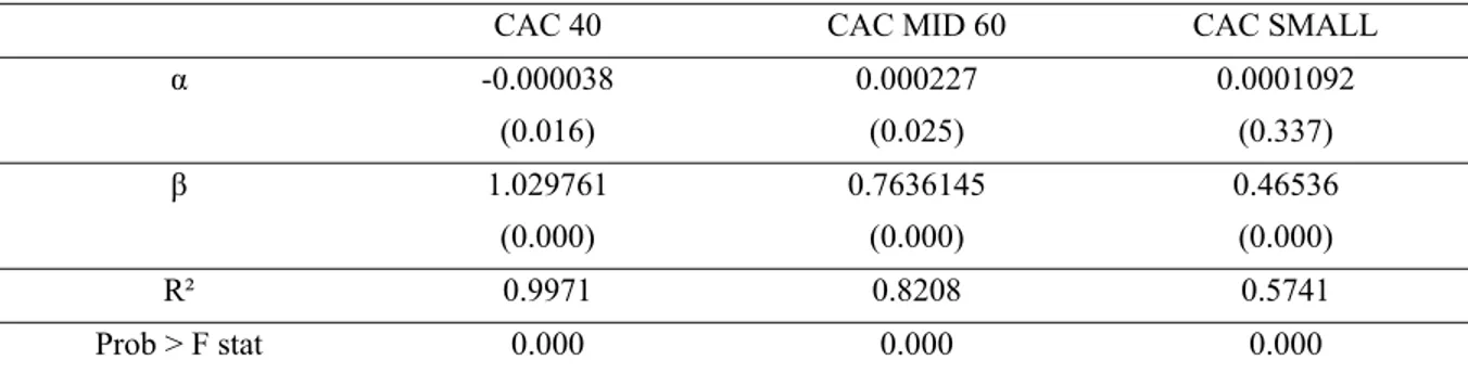
In this study, the CAC index shows that the performance of small and medium values is significantly greater than that of large ones between 2005 and 2016. This result presents a problem rin regards to the validity of the CAPM (see Table 3), according to which the expected yield of securities depends on the systematic risk level. We find that beta levels are not able to explain security return rates, as medium cap alpha is significantly greater than zero (0.0227%), and large alpha is significantly negative (-0.0038%).
Table 3. The unconditional CAPM
CAC 40 CAC MID 60 CAC SMALL
α -0.000038 (0.016) 0.000227 (0.025) 0.0001092 (0.337) β 1.029761 (0.000) 0.7636145 (0.000) 0.46536 (0.000) R² 0.9971 0.8208 0.5741 Prob > F stat 0.000 0.000 0.000
Notes: The p-values are shown in parentheses.
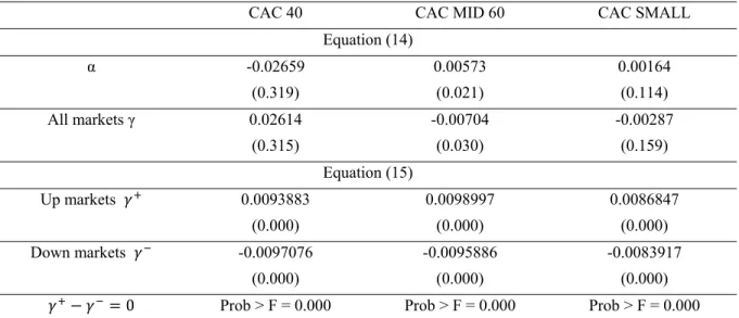
To produce an uncorrelated sequence from the return series, an autoregressive process is necessary. The author found an ARMA(1,1) process for the three indices. The residual series is strict white noise and shows no significant autocorrelation (Appendix A3 – A8). Beta estimation requires the conditional variance and the covariance, both of which are modeled as an ARCH process. Having estimated both the conditional variance and the conditional covariance, beta is then estimated in accordance with equation (12). Table 4 reports the results from the cross-sectional regression as given by equation (14), showing the average risk premium of the CAC index over the total time period, γ= 0.02614.
Morelli (2011) claimed that the positive risk premium implies a positive risk-return relationship. He noted that the insignificant beta can be explained by the aggregation of data during periods when excess market return is both positive and negative. The risk premium in our study is not statistically significant, so the hypothesis in which γ≠0 is
rejected, and beta doesn’t play a significant role in explaining security returns. Such findings are in accordance with studies on the US markets by Davis (1994) and Fama and French (1992) and the study on the UK market by Morelli (2011). Morelli (2011) noted that the insignificant beta can be explained by the aggregation of data during periods when excess market return is both positive and negative.
Table 4. The relationship between beta and returns, January 2005 to March 2016
CAC 40 CAC MID 60 CAC SMALL
Equation (14) α -0.02659 (0.319) 0.00573 (0.021) 0.00164 (0.114) All markets γ 0.02614 (0.315) -0.00704 (0.030) -0.00287 (0.159) Equation (15) Up markets 0.0093883 (0.000) 0.0098997 (0.000) 0.0086847 (0.000) Down markets -0.0097076 (0.000) -0.0095886 (0.000) -0.0083917 (0.000)
− = 0 Prob > F = 0.000 Prob > F = 0.000 Prob > F = 0.000
Notes: The table reports the time-series coefficients (risk premiums) in all markets and up and down markets, the p-values are shown in parentheses. A two-population F-test is shown examining the symmetry hypothesis between the risk premium − in up and down markets.
Table 4 presents the results from the equation 15 which tests the beta-return relationship conditional on the sign of the excess market return (Eq. (15)). This table also reports the average risk premium in both up and down markets. We find the cross-sectional regression show a significant positive relationship between beta and returns during up markets, and a significant negative relationship between beta and returns during down markets. According to this result, the null hypothesis of no beta-return relationship is rejected. The mean value of the regression coefficient for the CAC 40 index is 0.0093883, and the mean value of the regression coefficient for the CAC Mid is 0.0098997. This data implies that high beta portfolios exhibit higher returns during up markets than low beta portfolios.
The mean value of the regression coefficient for the CAC 40 index is -0.0097076, and the mean value of the regression coefficient for the CAC Mid is -0.0095886. Such findings imply that during down markets high beta portfolios earn lower returns than low beta portfolios. These results are in accordance with the findings of Morelli (2011), which suggest that beta risk is rewarded in up markets for losses incurred in down markets. This significant beta-return relationship is consistent across the total time period and also across both subperiods.
Pettengill et al. 1995 and Morelli 2011 posed that a conditional beta-return relationship does not ensure a positive risk-return relationship. The author has examined the risk premiums and from the Equation (15), the results of which can be found in Table 4. Over the whole period, a symmetrical relationship is found. We can conclude that there is a positive risk-return relationship in the French stock market.
5. Conclusion
According to our results, the estimated alphas are particularly significant for the CAPM model, the alpha of small and medium caps are slightly greater than zero and the alpha of large caps are negative. This confirms the link between the size effect and returns, though the security return rates cannot be explained by the beta levels.
The results of this study contribute to the existing literature regarding the role of beta in explaining security returns through the incorporation of ARCH models to estimate time varying betas. The empirical result, when we ignore the sign of the excess market return the beta is found to be an insignificant risk factor when the sign of the excess market return is ignored. During periods when the excess market return is positive, a significant positive relationship is
found between beta and returns. And during periods when the excess market return is negative, a significant negative relationship is found between beta and returns. This finding confirms the hypothesis of Pettengill et al. (1995) and Morelli (2011).
However, the conditional beta cannot be explained entirely by the size effect, the results show a positive relationship between beta and returns during up markets, so the risk premium of the small caps can not explain why the small caps have a better level of returns. It is important to investigate the relationship between conditional beta and the security returns in the equity markets of other countries.
References
Banz Rolf W. (1981). The Relationship between return and market value of common stocks. Journal of Financial Economics, 9.
Black, F., Jensen, M.C., & Scholes, M. (1972). The capital asset pricing model: some empirical tests. In Jensen, M.C. (Ed.), Studies in the Theory of Capital Markets (pp. 79–124). Praeger, NY.
Bollerslev, T. (1986). Generalized autoregressive conditional heteroscedasticity. Journal of Econometrics, 31, 307-327. http://dx.doi.org/10.1016/0304-4076(86)90063-1
Engle, R.F. (1982). Autoregressive conditional heteroscedasticity with estimates of the variance of the United Kingdom Inflation. Econometrica, 50, 987-1007. http://dx.doi.org/10.2307/1912773
Engle, R.F., Bali, T.G., & Tang, Y. (2013, February). Dynamic conditional beta is alive and well in the cross section of daily stock returns. Working paper 1305. Retrieved from http://papers.ssrn.com/sol3/papers.cfm?abstract_id=2089636&rec=1&srcabs=2078295&alg=1&pos=10
Engle, R.F., Jondeau E., & Rockinger M. (2012). Dynamic Conditional Beta and Systemic Risk in Europe. Retrieved from http://www.stern.nyu.edu/sites/default/files/assets/documents/con_037459.pdf
Fama E. F., & French K. R. (1992). The cross-section of expected stock return. The Journal of Finance, 47.
Fama E. F., & French K. R. (1995). Size and book to market factors in earnings and returns. The Journal of Finance, 50.
Hamon, J., & Jacquillat, B. (1992). Le marché français des actions: Etudes empiriques 1977-1991. PUF.
Horowitz, J.L., Loughran, Tim, & Savin, N.E. (2000). The disappearing size effect. Research in Economics, 54, 83-100. http://dx.doi.org/10.1006/reec.1999.0207
Jagannathan, R., & Wang, Z. (1996). The conditional CAPM and the cross-section of expected returns. Journal of Finance, 51, 3-53. http://dx.doi.org/10.1111/j.1540-6261.1996.tb05201.x
Kim, Moon K., &Burnie, D. A. (2002). The Firm Size Effect and the Economic Cycle. The Journal of Financial Research, XXV(1), 111-124.
L’Her, Masmoudi, Suret. (2002). Effet taille et Book-to-Market au Canada. Revue canadienne d’investissement. Été. Lewellen, J., & Nagel, S. (2006, January). The Conditional CAPM does not explain asset pricing anomalies. Journal
of Financial Economics. http://dx.doi.org/10.1016/j.jfineco.2005.05.012
Lintner, J. (1965). The valuation of risky assets and the selection of risky investments in stock portfolios and capital budgets. Review of Economics and Statistics, 47, 13–37. http://dx.doi.org/10.2307/1924119
Mathijs, A. van Dijk. (2011). Is Size Dead? A Review of the Size Effect in Equity Returns. Journal of Banking & Finance, 35(12), 3263-3274. http://dx.doi.org/10.1016/j.jbankfin.2011.05.009
Morelli, D.A. (2007). Conditional relationship between beta and return in the UK stock market. Journal of Multinational Financial Management, 17, 257–272. http://dx.doi.org/10.1016/j.mulfin.2006.12.003
Morelli, D.A. (2011). Joint conditionality in testing the beta-return relationship: Evidence based on the UK stock market. Journal of International Financial Markets, Institutions & Money, 21, 1-13. http://dx.doi.org/10.1016/j.intfin.2010.05.001
Pettengill, G., Sundaram, S., & Mathur, I. (1995). The conditional relation between beta and returns. Journal of Financial and Quantitative Analysis, 30, 101–116. http://dx.doi.org/10.2307/2331255
Reinganum, M. (1981). Misspecification of Capital Asset Pricing Empirical Anomalies based on Earnings Yields and Market Values. Journal of Financial Economics, 9.
-0 .1 0 0. 00 0. 10 0. 20 0. 30 Au to co rre la tio ns o f r1 _c arre 0 10 20 30 40 Lag Bartlett's formula for MA(q) 95% confidence bands
-0 .1 0 0. 00 0. 10 0. 20 Pa rt ia l a u to co rre la tio ns o f r1 _c a rre 0 10 20 30 40 Lag 95% Confidence bands [se = 1/sqrt(n)]
Reinganum, M. (1999). The Significance of Market Capitalization in Portfolio Management over Time. Journal of Portfolio Management, 25.
Ross S. (1976). The Arbitrage Theory of Capital Asset Pricing. Journal of Economic Theory, 13, 341-360. http://dx.doi.org/10.1016/0022-0531(76)90046-6
Schwert G. W. (2003). Anomalies and Market Efficiency, Chapter 15. In George Constantinides, Milton Harris & Rene M. Stulz (Eds.), Handbook of the Economics of Finance (pp. 937-972). North-Holland.
Sharpe, W. (1964). Capital asset prices: a theory of market equilibrium under conditions of risk. Journal of Finance, 19, 425–442. http://dx.doi.org/10.1111/j.1540-6261.1964.tb02865.x
Appendix Tables
Table A1. Summary statistics for CAC 40, CAC MID and CAC SMALL Index
Obs Mean Std. Dev. Skewness Kurtosis
CAC 40 2853 4172.31 821.08 0.524453 -0.56128
CAC MID 60 2853 6737.19 1274.31 0.071452 -0.43058
CAC SMALL 2853 6682.76 1402.61 0.338951 -0.03022
Table A2. Dickey-Fuller test for returns
Test statistic 1% critical
value 5% critical value 10% critical value p-value for Z(t)
CAC 40 -52.1122 -2.580 -1.950 -1.620 0.0000
CAC MID 60 -44.738 -2.580 -1.950 -1.620 0.0000
CAC
SMALL -39.958 -2.580 -1.950 -1.620 0.0000
Table A3. Phillips-Perron test for returns
CAC 40 CAC MID 60 CAC SMALL 1% critical value
Z(rho) -2361.877 -2129.515 -2151.872 -13.800
Z(t) -52.619 -44.613 -40.820 -2.580
MacKinnon approximate p-value for Z(t) = 0.0000
Figures
-0 .1 0 -0 .0 5 0. 00 0. 05 0. 10 A ut oc o rr ela tion s o f e1 0 10 20 30 40 Lag Bartlett's formula for MA(q) 95% confidence bands
-0 .1 0 -0 .0 5 0. 00 0. 05 P ar tia l au to co rr e la tions of e 1 0 10 20 30 40 Lag 95% Confidence bands [se = 1/sqrt(n)]
-0 .0 5 0. 00 0. 05 Au to co rr el ati o ns o f e _a rm a 0 10 20 30 40 Lag Bartlett's formula for MA(q) 95% confidence bands
-0 .0 5 0. 00 0. 05 Pa rt ia l a u to co rre la tio ns of e _a rma 0 10 20 30 40 Lag 95% Confidence bands [se = 1/sqrt(n)]
-0 .1 0 0. 00 0. 10 0. 20 0. 30 A ut oc o rr el at io ns of e _ar m a 2 0 10 20 30 40 Lag Bartlett's formula for MA(q) 95% confidence bands
-0 .1 0 0. 00 0. 10 0. 20 0. 30 P ar tia l a u to co rr e lat io ns o f e_ ar m a2 0 10 20 30 40 Lag 95% Confidence bands [se = 1/sqrt(n)]
Figure A3. AC of res. CAC 40 Figure A4. PAC of res. CAC 40
Figure A5. AC of res. mean eq. CAC40 Figure A6. PAC of res. mean eq. CAC40