HAL Id: hal-00441026
https://hal.archives-ouvertes.fr/hal-00441026
Submitted on 10 Feb 2010
HAL is a multi-disciplinary open access
archive for the deposit and dissemination of sci-entific research documents, whether they are pub-lished or not. The documents may come from teaching and research institutions in France or abroad, or from public or private research centers.
L’archive ouverte pluridisciplinaire HAL, est destinée au dépôt et à la diffusion de documents scientifiques de niveau recherche, publiés ou non, émanant des établissements d’enseignement et de recherche français ou étrangers, des laboratoires publics ou privés.
To cite this version:
Pavel Kuzhir, Modesto Lopez-Lopez, Georges Bossis. Abrupt contraction flow of magnetorheolog-ical fluids. Physics of Fluids, American Institute of Physics, 2009, 21 (5), pp.053101.1-053101.13. �10.1063/1.3125947�. �hal-00441026�
Abrupt contraction flow of magnetorheological fluids
P. Kuzhir1, M.T. López-López1,2 and G. Bossis1
1
Laboratoire de Physique de la Matière Condensée, CNRS UMR 6622 Université de Nice, Parc Valrose, 06108 Nice Cedex 2, France
2
Departamento de Fisica Aplicada, Facultad de Ciencias, Universidad de Granada, 18071 Granada, Spain
Abstract
Contraction and expansion flows of magnetorheological fluids occur in a variety of smart devices. It is important therefore to learn how these flows can be controlled by means of applied magnetic fields. This paper presents a first investigation into the axisymmetric flow of a magnetorheological fluid through an orifice (so-called abrupt contraction flow). The effect of an external magnetic field, longitudinal or transverse to the flow, is examined. In experiments, the pressure-flow rate curves were measured, and the excess pressure drop (associated with entrance and exit losses) was derived from experimental data through the Bagley correction procedure. The effect of the longitudinal magnetic field is manifested through a significant increase in the slope of the pressure-flow rate curves, while no discernible yield stress occurs. This behavior, observed at shear Mason numbers 10 <Mnshear<100, is interpreted in terms of an enhanced extensional response of
magnetorheological fluids accompanied by shrinkage of the entrance flow into a conical funnel. At the same range of Mason numbers, the transverse magnetic field appears not to influence the pressure drop. This can be explained by a total destruction of magnetic particle
aggregates by large hydrodynamic forces acting on them when they are perpendicular to the flow. To support these findings, we have developed a theoretical model connecting the microstructure of the magnetorheological fluid to its extensional rheological properties and predicting the pressure-flow rate relations through the solution of the flow equations. In the case of the longitudinal magnetic field, our model describes the experimental results reasonably well.
I. Introduction
Magnetorheological (MR) fluid is a suspension of superparamagnetic micron-sized non-Brownian particles dispersed in a liquid carrier. In the absence of an external magnetic field, these particles have a zero magnetic moment and the MR fluid behaves as a conventional particulate suspension and follows a Newtonian rheological law at small – to moderate concentrations. When an external magnetic field is applied, the MR fluid particles become magnetized and attract each other forming chain-like aggregates aligned preferably in the direction of the magnetic field. Spanning the gap of a flowing channel, these aggregates block the MR fluid motion, and a yield stress must be applied to set up the flow. This phenomenon, referred to as magnetorheological effect (Shulman and Kordosky1, Bossis et al.2) has recently found commercial applications in smart technologies such as active car suspension (Carlson et al.3) and magnetorheological finishing (Kordonski and Jacobs4). Besides providing a high engineering interest, the MR fluids are very attractive from a purely scientific point of view. The coupling between field-induced structuring and hydrodynamic interactions gives rise to rich phenomena in MR fluid flows. Shear-induced nematic-to-isotropic transitions (Volkova et al.5), the formation of honeycomb and foam structures in triaxial magnetic fields (Martin et al.6), the distortion of the axial symmetry of pipe flows (Kuzhir et al.7) are a few examples of these phenomena.
If shear, squeeze and pipe flows of MR fluids have been thoroughly studied and are well documented in literature (reviews by Shulman and Kordosky1, Bossis et al.2 and Shulman8), there is no detailed and systematic study of the flows in converging geometries. Such flows occur in a variety of MR fluid smart devices such as active dampers, MR valves, MR finishing devices, active fluid bearings. In order to improve the performance of these devices, it is important to learn how these flows can be controlled by means of applied magnetic
fields. Besides the practical interest, contraction flow offers a good opportunity to test the extensional rheology of MR fluids, which is itself a completely new study. In a few known works on extensional flows of magnetic suspensions (Pérez-Castillo et al.9 and John et al.10), the rheological properties of the suspensions have not been analyzed. Thus, the objectives of the present paper can be summarized as follows: (1) an experimental and theoretical study of the magnetic field effect on the abrupt contraction flow of a MR fluid; (2) the analysis of the extensional rheological response of the MR fluid in contraction flow.
The experiments consist of squeezing an MR fluid through a small orifice and measuring the pressure difference between the two extremities of the flow channel as function of the flow rate. The pressure losses in the upstream and downstream channels (so-called excess pressure drop) are then deduced from the total pressure difference by Bagley correction procedure. The main result of our study is the dependence of the excess pressure drop on the flow rate in the presence of a magnetic field. In the vicinity of the orifice, the fluid experiences a strong stretching deformation, so-called extensional flow, and the excess pressure drop is partially attributed to normal viscous stresses in extensional flow. To extract the extensional rheological properties of MR fluid from the experimental pressure-flow rate curves, we must know, at least, the velocity profile in contraction flow. Instead of doing so, we evaluate theoretically these extensional properties and, based on this, we calculate the excess pressure drop. Concretely, we first derive a theoretical relation between the normal stress and extensional rate assuming a chain-like structure of the MR fluid. The above rheological relation is then integrated into a momentum equation, which is solved for a contraction flow of MR fluid and, thus, the excess pressure drop is calculated and fitted to experimental results. The comparison of theoretical and experimental excess pressure drops allows us to conclude on the magnetic field effect on the extensional viscosity of the MR fluid.
We must notice that the contraction flow is widely used in extensional rheology of polymers (Boger11, White et al.12). Furthermore, this method, also called “entry flow method”, is considered as the most appropriate one for the extensional rheology of low-to-moderate viscosity fluids, as, for example, particulate suspensions (Macosco13).
Because of the field-induced chain formation in MR fluids, their contraction flow is expected to possess some features of the contraction flow of fiber suspensions. Contraction flows of conventional fiber suspensions have been the subject of numerous papers. Mongruel and Cloitre14,15, Cloitre and Mongruel16 have performed simultaneous flow visualization and measurements of the pressure – flow rate relation for the fiber suspensions flowing through a small circular orifice introduced into a wide cylindrical channel. Upstream of the orifice, the flow is extensional, the fibers are oriented along the flow lines and generate large extensional stresses. A large corner vortex with recirculation flow is observed, the main entrance flow is therefore concentrated in a central funnel. With a growing fiber aspect ratio, the extensional viscosity of the fiber suspension increases, which enhances the corner vortex and shrinks the funnel of the main flow. Thus, the pressure loss in the upstream channel (entrance pressure drop) appears to be a growing function of the fiber length. The vortex enhancement and the increase in the pressure loss also take place downstream of the orifice, unless the fibers are oriented perpendicular to the flow. In their papers, Mongruel and Cloitre give a simple analytical model predicting the entrance and the exit pressure losses for fiber suspensions.
By analogy with fiber suspensions, MR fluids could also develop some recirculation or dead corner zones. The main flow is expected to get narrower with the magnetic field growth because the fibrous aggregates get longer and generate higher extensional stresses. So, the excess pressure drop is expected to be a growing function of the magnetic field intensity.
The particularities of MR fluid contraction flows are analyzed in the present paper, which is organized as follows. First, we present the experimental procedure followed by the experimental results on the pressure – flow rate relation for an abrupt contraction flow of an MR fluid in the presence of a magnetic field parallel and transverse to the channel axis. In the final section, we develop a theoretical interpretation of the results for the axial magnetic field. The theoretical predictions are tested against experiments and discussed in the light of the further development of the MR fluid extensional rheology.
II. Experimental procedure
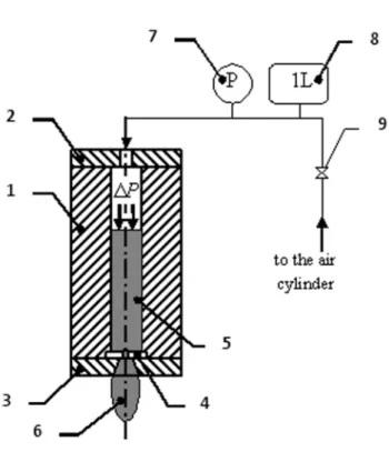
The experimental flow cell is shown in Fig. 1. It was composed of a plexiglass cylindrical tube, 50 mm in length and 5 mm in internal diameter, and two brass lids attached to both lateral faces of the plexiglass tube. The lower lid had a central tapered hole; a thin disk (made of titanium sheet, Goodfellow) with a coaxial cylindrical orifice was glued to the upper side of the lid. Disks of two different thicknesses were used: 0.1±0.01 mm and 0.5±0.01 mm and the orifice diameter was 0.32±0.01 mm. The MR fluid initially filled the whole flow cell. Under gravity, the fluid did not flow away through the orifice (at least during typical experimental time) because of its relatively high viscosity (3.4 Pa·s). The upper lid of the cell was connected to a compressed air cylinder through a precision control valve. The valve allowed us to impose the relative pressure in the range 0.25 – 5 bars with a precision of ±0.02 bars. The applied pressure was measured by a piezoelectric pressure transducer (Parker Filtration UCC, ref. PTD.010821, accuracy ±0.02 bar) placed in the air circuit upstream of the flow cell. The cell was sealed by two polyvinyl rings placed on the contact surface between the plexiglass tube and the lids.
Fig. 1. Experimental flow cell. 1 – plexiglass tube; 2 – upper brass lid; 3 – lower brass lid; 4 – thin titanium disk with a coaxial orifice, 0.3 mm in diameter; 5 – MR fluid; 6 – hanging MR fluid drop; 7 – pressure transducer; 8 – air reservoir, 1L; 9 – precision control valve. Helmholtz coils and electronic balance are not shown in the schema.
Once the pressure was applied, the MR fluid flowed through the orifice and dripped onto a collector placed on the top of the electronic balance Denever Instrument MXX123 (accuracy ±1 mg). The mass, M, of the collected fluid was measured during the time t, and the instantaneous value of the volumetric flow rate was calculated as Q(t)=∆M/(
ρ
∆t) withρ
=1.65g/cm3 being the MR fluid density. The level of the MR fluid in the flow cell decreased as the fluid flowed through the orifice and we stopped the mass measurements when the level became ¼ of the initial one. The air reservoir, 1L in volume, was introduced between the precision valve and the flow cell and allowed the air pressure to be kept constant during experiments. In every experimental case, we checked that the flow rate relaxed very quickly to a steady value after the application of pressure. So, the measurement of the pressure – flowrate curve was organized as follows. The flow cell was completely filled with the MR fluid; a given pressure was applied and a corresponding flow rate was measured. Then the flow cell was cleaned from MR fluid and the orifice was washed with alcohol and acetone and blown out by compressed air. The flow cell was again filled with the MR fluid and the measurement was repeated with another value of applied pressure. Measurements for the same applied field and pressure were repeated in order to check reproducibility.
The total applied pressure drop (the pressure difference between the upper and lower free surfaces of the MR fluid) is conventionally divided into two parts – the Poiseuille pressure drop due to the Poiseuille flow through the thin orifice and the excess pressure drop due to the flow contraction at the orifice entry and expansion at the orifice exit: ∆Ptot = ∆PPois + ∆Pexcess. Each pressure loss component is shown in Fig. 7c where a pressure profile along the
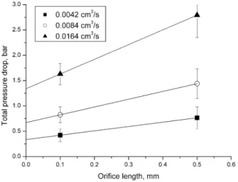
flow cell is illustrated schematically. In our experiments we are more interested in the excess pressure drop, also called Bagley correction, because it is directly connected to the extensional stresses in the MR fluid. In order to extract the excess pressure drop from experimental data, we apply the Bagley correction to the experimental data (Bagley17, Macosco13), i.e. we plot the total pressure drop versus the orifice length, ∆Ptot(L), for a given
value of the flow rate (as show in Fig. 5) and define the excess pressure drop as a linear extrapolation of the ∆Ptot(L) curve onto zero orifice length: ∆Pexcess= ∆Ptot(0). Having found
the Bagley correction for each value of the flow rate, we plot the dependencies of the excess pressure drop versus the flow rate, which is the principle experimental result of our study allowing us to analyze the extensional rheological properties of the MR fluid as well as the magnetic field effect on these properties.
All the measurements discussed above were carried out in the absence and in the presence of an external uniform magnetic field, parallel or perpendicular to the flow cell axis. The
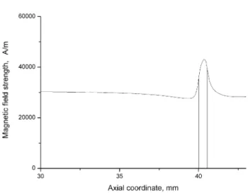
magnetic field was created by a pair of Helmholtz coils placed around the channel. These coils provided the magnetic field intensity in the range of 0 – 30.6 kA/m. The Helmholtz coils were sufficiently large compared to the flow cell. So, the non-uniformity of the created magnetic field was maximum 1% in the air space where the flow cell was introduced. Due to the demagnetizing effect, the uniformity of the magnetic field was distorted inside the MR fluid sample. We carried out numerical simulations by finite element method of the internal magnetic field in the case of the applied external axial field H0=30.6 kA/m. The magnetic
field distribution along the flow cell axis in the downstream direction is shown in Fig. 2. The magnetic field strength appears to be uniform and close to the strength of the external field in the major part of the flow cell. But in the vicinity of the orifice, the magnetic field grows from H≈30 kA/m at a distance 5 mm from the orifice, to H=35.7 kA/m at the orifice entrance and reaches its maximum H=43 kA/m inside the orifice. The calculation of exact magnetic field distribution in the transverse field would require the solution of a 3D Maxwell equation problem. To avoid this difficulty, we estimate the internal transverse magnetic field as the field inside an infinitely long cylinder with the demagnetizing factor ½:
0/ 1 12( 1)
H =H +
µ
− . Here,µ
≈1.55 is the MR fluid relative magnetic permeability. So, in the presence of the external magnetic field, transverse to the channel axis, of an intensity H0=25 kA/m, the internal magnetic field is H≈20 kA/m.Fig. 2. Distribution of the magnetic field strength along the flow cell axis in the downstream direction. The orifice length is L=0.5mm. Two vertical lines indicate the orifice position
The MR fluid used in our experiments was a suspension of carbonyl iron particles (BASF), ranging from 0.5 to 3 microns in diameter, dispersed in a homogeneous mixture of the silicon oil Rhodorsil® 47V500 (VWR Prolabo) and the Brookfield 60000 oil. This oil mixture appeared to be a Newtonian fluid with a viscosity
η
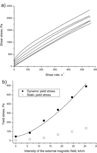
0=2.5 Pa·s. The volume fraction of particles in suspension, Φ, was fixed to 10%. In order to avoid the particle aggregation under colloidal forces, the MR fluid was stabilized by a surfactant - aluminum stearate (Sigma Aldrich, 6.15 g/L), following the method described in details in López-López et al.18. The shear rheological properties of the MR fluid were measured using a controlled-stress rheometer Haake 150 RS in a cone-plate geometry with diameter 35 mm and angle 2°. An external uniform magnetic field, of intensity 0 – 30.6 kA/m, was applied perpendicular to the measuring gap by a solenoid placed around the cone-plate geometry.The results of the MR fluid shear rheometry are shown in Fig.3. At shear rates, γ& >150 s-1, the MR fluid flow curves were almost linear and approximated by the Bingham rheological
law:
τ
=τ
D+η
⋅γ
&, with a dynamic yield stress,τ
D, defined by a linear interpolation of theflow rate curve onto zero shear rate (Fig. 3a). The dynamic yield stress was found to be a power law function of the applied magnetic field intensity, H0: 0 0
n
D D H
τ −τ ∝ , with n=1.31±0.13. Such field dependence of the yield stress is close to the 3
2-power law predicted by Ginder et al.19:
1/ 2 3/ 2 1/ 2 3/ 2 0 0 0 3/ 2 0 0 6 6 D D MS H D MS H τ τ µ τ µ µ ⋅Φ = + ⋅Φ ⋅ = + ⋅ , (1)
where µ0=4π·10-7 H/m is the magnetic permeability of vacuum, MS=1.36·106 A/m is the
saturation magnetization of carbonyl iron particles (de Vicente et al.20, Bossis et al.2), H=H0/µ is the magnetic field intensity inside the MR fluid sample and τD0≈45 Pa is the MR
fluid dynamic yield stress at zero field. Such non-zero dynamic yield stress at zero field could come from colloidal interactions between particles and is introduced into the Ginder’s equation (1) as an additive constant.
So, the experimental points are well fitted by the equation (1) (solid line in Fig.3b) with a numerical coefficient multiplying µ0MS1/ 2H03/ 2equal to 0.074±0.02 instead of
3/ 2
6⋅Φ/µ ≈0.127. The static yield stress was defined as a shear stress plateau at the inception of the flow curve plotted in logarithmic scale (cf. Barnes21, Malkin22). It was also found to be a growing function of the magnetic field but was a few times smaller than the dynamic one (Fig.3b).
Fig. 3. Shear rheometry of the MR fluid in the presence of the magnetic field normal to the flow: flow curves (a) at different magnetic field intensities; the yield stress versus the magnetic field intensity (b). In figure (a), the flow curves correspond to the magnetic field intensity, varying from the lower to the upper curve: H0= 0, 6.1,
12.2, 18.3, 24.4 and 30.6kA/m. The solid line in figure (b) is a fit of the experimental dynamic yield stress by the equation (1).
To inspect the inertia effects, the Reynolds number, Re=ρvX/η, was estimated in the scale of the flow cell and in the particle scale: 0.01<Reorifice<0.1 and 0.0003<Repart<0.003,
respectively. Here v=Q/(
π
R02)is the average MR fluid velocity at the orifice,η
=3.4 Pa·s is the MR fluid viscosity at the shear rateγ
& >100 s-1, X corresponds to either the orifice diameter (2R0=0.3 mm) or the particle diameter (2a≈1 µm). The Reynolds number wascalculated for the experimental range of the flow rates, 0.005<Q<0.05 cm3/s. Because of the low Reynolds numbers, the MR fluid flow is considered to be laminar both in the flow cell and around the particles.
In order to check the validity of our measurements, we tested our experimental cell with two calibrated Newtonian oils with viscosities
η
=0.485 Pa·s (silicon oil Rhodorsil® 47V500; VWR Prolabo) andη
=2.5 Pa·s (homogeneous mixture of the Rhodorsil® 47V500 oil with Brookfield 60000 oil). The measured total pressure drop was separated into the Poiseuille pressure drop and the excess pressure drop by applying the Bagley correction, and both experimental curves, ∆PPois(Q) and ∆Pexcess(Q), were compared with the correspondingtheoretical dependencies: Q R L PPois 4 0 8
π
η
= ∆ , (2) Q R Pexcess 3 0 3η
= ∆ , (3)where L = 0.1±0.01 or 0.5±0.01 mm is the orifice length. The formula (3) expresses the pressure drop for the creeping flow through an infinitely short circular orifice and is recommended for estimations of the entrance and exit pressure losses in the pipe flows at low Reynolds numbers (Happel and Brenner23, Weissberg24). Note that the pressure losses predicted by eq. (3) are symmetric about the orifice plane, i.e. the entrance and the exit pressure losses are the same and equal to a half of the excess pressure drop (3).
We found that the experimental curves ∆PPois(Q) and ∆Pexcess(Q) for the calibrated oils were
theoretical curves (2) and (3): ∆PPois/Q=8ηL/(πR04) and ∆Pexcess/Q=3 /η R03. Such discrepancy could occur due to a small fluid inertia effects near the orifice edges.
III. Experimental results
The dependencies of the total pressure drop versus flow rate are shown in Figs. 4a, b for the orifice lengths, L=0.1 mm and 0.5 mm, as well as in the presence and in the absence of the magnetic field. In all experimental cases, the ∆Ptot(Q) – relation appears to be linear. The
effect of the axial magnetic field is manifested through an increase in the pressure drop at the same flow rate (Figs. 4a, b). The total pressure drop is found to be directly proportional to the flow rate: ∆Ptot ∝Q, and, within the experimental error, we do not find any distinguishable
yield pressure drop, even at the magnetic field as high as H0=30.6 kA/m. But, at the same
field intensity, the slope of the ∆Ptot(Q) curve is 2.4 and 3 times higher than the slope at zero
field for the orifice of the length 0.1 mm and 0.5 mm, respectively. This behavior could be identified with zero or very low yield stress and with enhanced MR fluid viscosity in contraction flows and is discussed in detail at the end of this section.
Fig.4. Total pressure drop versus the flow rate for the orifice length 0.1 mm (a) and 0.5 mm (b). Lines represent a linear fit to the experimental data.
There is no distinguishable effect of the transverse magnetic field on the pressure – flow rate characteristics of the MR fluid. Experimental points for the intensity of the external magnetic field H0=4 kA/m and 25 kA/m (intensity of the internal field is H=3.1 kA/m and 20kA/m,
respectively) gather, within experimental error, along the straight line corresponding to zero field (Figs. 4a,b). This result could be explained by the total destruction of MR aggregates and is discussed in more detail at the end of this section. Thus, in contraction flows, the axial magnetic field generates a rather strong growth in the slope of the ∆Ptot(Q) curve (hydraulic
is opposite to that found in shear flows or pipe flows (Shulman and Kordonsky1, Kuzhir et al.7, Takimoto et al.25), at least at high Masson numbers. Note finally that both in the transverse and zero magnetic field, the yield pressure drop is nonzero, even though it is small compared to the experimental pressure range: ∆PY=0.163±0.073 bar for the orifice length 0.1
mm and ∆PY=0.283±0.035 bar for the orifice length 0.5 mm. Such apparent yield pressure
drop is defined as an intercept of the ∆Ptot(Q)–curve interpolated linearly until zero flow rate
and is associated to a shear thinning behavior of the MR fluid at small flow rates.
In Fig. 5, we present an example of Bagley plot made for the axial magnetic field of an intensity, H0=30.6 kA/m. The similar plots were done for all experimental data and the excess
pressure drop was determined as described in the previous section. By doing so, we supposed that, in the presence of a magnetic field, the entrance pressure drop could be decoupled from the Poiseuille pressure drop in the same way as at zero field. This assumption requires verification by numerical simulations of the abrupt contraction flow.
Fig. 5. Bagley plot for the MR fluid contraction flow at various flow rates and in the presence of axial magnetic field of intensity, H0=30.6 kA/m.
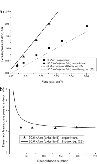
Experimental dependence of the excess pressure drop versus the flow rate is shown in Fig. 6a for zero magnetic field as well as for the axial field of an intensity, H0=30.6 kA/m. Similar to, ∆Ptot(Q) curves, the ∆Pexcess(Q) curves are linear and the slope is 2.3 times larger in the
presence of the field than at zero field. The dashed line in Fig. 6a corresponds to the theoretical ∆Pexcess(Q) dependence for zero magnetic field calculated by the eq. (3). We see
that the experimental dependence for zero field is well parallel to the theoretical one but slightly shifted upwards by 0.13 bars. This discrepancy might be due to a slight Bingham behavior of MR fluids in the absence of field, as discussed above.
The solid line in Figs. 6a is a theoretical pressure – flow rate relation corresponding to the axial magnetic field, H0=30.6 kA/m, and derived in the next section. Qualitatively, the
magnetic field effect on the contraction flow of MR fluids can be interpreted in the following manner.
Fig. 6. Dimensional (a) and dimensionless (b) dependencies of the excess pressure drop versus the flow rate in the absence and in the presence of a magnetic field axial to the channel axis, H0=30.6 kA/m.
When an axial magnetic field is applied, it creates chain-like clusters composed of magnetic particles and aligned with the magnetic field lines. When the MR fluid flows through a contracted channel, these chains move together with the fluid and are subject to a complex velocity field. Upstream of the orifice, along the channel axis, the flow is extensional because the MR fluid accelerates when approaching the orifice. Both the extensional flow and the axial magnetic field orient the chains along the channel axis. These chains are subject to tensile hydrodynamic forces proportional to the extensional rate, which varies significantly from very low values, of the order,
ε
&∝Q/(π
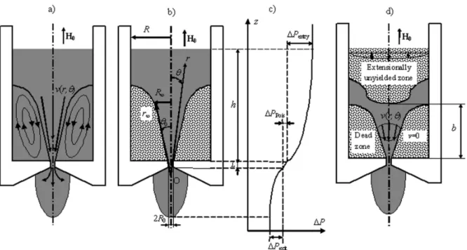
R3)∝0.1÷1 s-1, far upstream of the orifice to high values, ε&∝103÷104 s-1, at the orifice entrance. Thus, the chains may be destroyed inthe vicinity of the orifice but can sustain the tensile deformations at some distance away from the orifice. The chain length and the extensional viscosity are expected to be a growing function of the distance from the orifice in the upstream direction. A key assumption of the present work is that the main entrance flow is confined in a narrow conical funnel separated from the channel wall by a stagnant (recirculating or non-flowing) fluid, as shown in Fig.7a,b. One of the possible reasons for the funnel flow is a large extensional viscosity of the MR fluid in the presence of the longitudinal magnetic field. Being subject to a strong elongation, the entry flow shrinks into a funnel, and a large recirculation zone appears at the channel corners (Fig. 7a), in the same way as for the contraction flows of polymers or fiber suspensions (Boger11, Mongruel and Cloitre14). If the recirculation is not intense enough in the presence of the magnetic field, the fluid motion could stop within this zone and the corner vortex likely transforms to a solid plug as shown in Fig. 7b. The entrance pressure loss for the funnel flow appears to be much higher than that for a creeping Newtonian flow with a small corner vortex. This could explain why the pressure loss in the longitudinal magnetic field is larger than in the absence of field.
Such behavior in the axial magnetic field can be better reflected by the dimensionless pressure-flow rate dependence, shown in Fig. 6b. The excess pressure drop is normalized by
the one in the absence of magnetic field, 3 0 3 ) 0 ( R Q Pexcess
η
=∆ , and the flow rate is replaced by the shear Mason number2 – characteristic ratio of hydrodynamic – to – magnetic forces,
2 0 2 0 0 8 H Mnshear
β
µ
γ
η
&= , where
γ
&=4Q/(π
R03) is the apparent wall shear rate at the orifice,β
=(µ
p–1)/(µ
p+2)≈1 andµ
p>>1 is the relative magnetic permeability of carbonyl ironparticles. In experiments, the dimensionless pressure drop appears to be independent of Mason number, within the range, 30<Mnshear<200. This can be explained as follows. The
entrance pressure drop has two contributions: one related to the solvent shear stress and the second to the stresses generated by particle chains. The chains are aligned with the stream-lines and, perhaps, give a moderate contribution to the pressure drop. The solvent contribution depends strongly on the apex angle of the funnel, and the apex angle appears to be independent of Mason number in the interval, 30<Mnshear<200. From the theoretical point
of view, our model (solid line in Fig. 6b) predicts the dimensionless pressure drop to be inversely proportional to Mason number: ∆Pexcess(H) /∆Pexcess(0)= + ⋅A B Mnshear−1 (section IV.2). At Mason numbers, Mnshear>100, the second term vanishes and the dimensionless
pressure drop becomes independent of Mason number, as in experiments. At lower Mason numbers, the theory predicts a non-negligible effect of the magnetic field on the extensional stress generated by chains, so the dimensionless pressure drop increases with decreasing Mason numbers (or increasing magnetic field).
Fig. 7. Geometry of the abrupt contraction flow in the presence of a magnetic field axial to the channel axis. Either a large vortex (a) or a dead zone without any flow (b) are expected in the corner of the upstream channel. This dead zone could appear because of field-induced aggregation of the MR fluid. In both cases (a) and (b), the MR fluid flows through a narrow funnel with a small half-apex angle, θ0. Spherical coordinate system (r,θ,φ) is
introduced together with an apex point O in figure (b). A schematic pressure profile along the channel axis is shown in figure (c) and each term contributing to the total pressure drop is represented. An extensionally
unyielded flow region is illustrated schematically in figure (d). The extensional rate vanishes within this zone while the shear rate is finite and non-homogeneous.
In the transverse magnetic field, the structure of the MR fluid entrance flow should not be the same, as in the case of the longitudinal field. The transverse field forms the chains of magnetic particles in the direction perpendicular to the main flow. The chains rotate under the action of the hydrodynamic torque and can be easily destroyed by the tensile hydrodynamic forces. This is especially expected in our experimental case of high shear Mason numbers Mnshear≈10÷100. So, in the transverse magnetic field, the MR fluid behaves as a conventional
suspension of individual particles. Since the MR fluid does not show an enhanced extensional response in the transverse field, the corner vortex, if it exists, should be as small as in the absence of the magnetic field. Otherwise, if a solid plug is formed instead of vortex, the stagnation zone is also expected to be small compared to that in the longitudinal field because the field-induced aggregation is more effective in the longitudinal field. So, in the transverse magnetic field at 10<Mnshear<100, the flow is not restricted to a funnel, and the entrance
pressure drop is field-independent.
Note as well that, if, in the transverse magnetic field, the particle aggregation seems to be impossible at Mason numbers as high as Mnshear≈10÷100, there is no such evidence for the
longitudinal field. This is because the MR aggregates are aligned with the flow in the longitudinal field and are not subject to shear deformation but rather to extensional deformation. In this case, the existence of aggregates is defined rather by extensional Mason number, which is a characteristic ratio of the hydrodynamic stretching force in extensional
flow to the magnetic force between particles: 2 0 2 0 0 8 H Mnext
β
µ
ε
η
&= . We shall see in the Section IV.2 that the extensional rate, ε& is an order of magnitude lower than the shear rate, γ& , so the
Recall, finally, that the internal longitudinal magnetic field in the MR fluid inside the orifice is about two times higher than the internal transverse field at nearly the same external field. Such a demagnetizing effect should influence the pressure drop but is not strong enough to explain a 3-times increase in pressure drop in the longitudinal field and the absence of the MR effect in the transverse magnetic field.
IV. Theory and discussion
In this section we develop a theoretical model predicting the dependence of the entrance pressure drop versus the flow rate in the presence of the longitudinal magnetic field. This theoretical dependence is then fitted to experimental results and the free parameter – apex angle of the funnel is deduced from this fit. The model consists of the rheological part (section IV.1) and the fluid mechanics part (section IV.2). In the first part, a relation between the normal stress and extensional rate is derived using Bachelor’s slender body theory and assuming a chain-like structure of the MR fluid. This relation appears to be the first theoretical law in extensional rheology of MR fluids. In the second part, the above rheological relation is integrated into a Cauchy momentum equation, which is solved for a contraction flow of MR fluid and, thus, the excess pressure drop is calculated and fitted to experimental results.
IV.1. Uniaxial extension
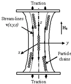
In order to derive a relation between the normal viscous stresses and extensional rate, we shall consider a homogeneous extensional flow, which can be realized by stretching a fluid column with a speed increasing exponentially with time (Macosco13). Such flow is shown
schematically in Fig. 8 and is characterized by a linear velocity profile as follows: vx x 2 ε& − = ; y vy 2 ε& −
= and vz =+
ε
&⋅z. The rate-of-strain tensor is diagonal and its components are2
ε ε
εxx = yy =− & and
ε
zz =ε
&. Heredz dvz
≡
ε& is the extensional rate; the Cartesian reference system, Oxyz, is chosen in such a way that the z-axis is parallel to the extension axis while x- and y-axes are transverse to the extension axis. Suppose that an external magnetic field, of intensity H0, is applied along the z-axis. The central stream-line (on the z-axis) is therefore
parallel to the central field line while the periphery stream-lines (out of the z-axis) cross the field lines at some, generally small, angle.
Fig. 8. Uniaxial extension of the MR fluid in the presence of a magnetic field parallel to the extension axis. The particle chains are approximately aligned with the stream-lines and subject to both the hydrodynamic tensile and the magnetic attractive forces.
In this subsection, we intend to find the extensional extra-stress generated by the magnetic particles in the extensional flow. First, we need to introduce the following hypotheses:
1. The magnetic field induces MR fluid aggregation, and, at the first approximation, the aggregates are supposed to be single straight chains with no interaction between them.
2. As already stated, the extensional flow tends to orient the chains along the stream-lines and the magnetic field tends to align them with the field lines. The chains therefore are oriented at a certain angle between the velocity lines and the field lines. Due to the flow geometry (Fig. 8), this angle should be quite small in the major part of the flow, and, thus, it can be considered that all the particle chains are aligned with the flow lines. The field is also considered to be parallel to the chains. This assumption will significantly simplify calculations of the particle stress and will affect the results by a minor relative error, of the order of
α
2, withα
– the angle between velocity lines and chains.3. Under hydrodynamic tensile forces, the chains break in their center and form two identical chains. In steady conditions, all the chains are assumed to have the same length defined by the balance between the hydrodynamic tensile force and magnetic attractive force between two central particles.
4. The chains length, 2l, is much higher than the particle diameter, 2a, but much lower than the characteristic length, L, of the flow cell: 2a<<2l<<L. The left inequality suggests low Mason numbers, i.e. high magnetic fields and/or low extensional rates.
5. The Batchelor’s26,27 slender-body theory is employed for the long chains in extensional flow. At first approximation, we consider dilute suspensions of chains which imposes the restriction on the concentration of the MR fluid: Φ<<(a/l)2. From Batchelor’s theory the
following formulas are derived for the tensile force exerted by the solvent per unit chain length (4), the extra stress tensor (5) and extensional stress components (6), (7):
ξ
ε
πη
& ) / 2 ln( 2 0 a l fh = (4) 0 1 2 3 ik ik ch n n n ni k l m ikn nl m lm τ = η ε +η − δ ε & & (5) ε η η τ τ & + − = = yy ch xx 3 1 0 (6) ε η η τ & + = ch zz 3 2 0 (7)In these formulae, η0 is the solvent viscosity, ξ is the distance along the chain axis from its
center, n is the unit vector along the chain axis, ε& is the rate of strain tensor, ik δik is the Kronecker delta, ηch is the viscosity coefficient associated with viscous friction due to the
presence of chains: ) / 2 ln( ) / ( 3 2 2 0 a l a l ch ch
η
η
= Φ (8)with Φch≈Φ being the volume fraction of chains in MR fluid and Φ - the volume fraction of
magnetic particles.
The chains experience the maximal tensile force, Fh, in their center, and this force is obtained
by integration of the force density (4) over the chain length:
) / 2 ln( d 2 0 0 l a l f F l h h
ε
πη
ξ
= & =∫
(9)The magnetic force between two touching central particles of the chain is proportional to the particle cross-section,
π
a2: 2 ( ) m m F = f ⋅ πa , (10)where fm is the magnetic force per unit particle cross-section. This force depends on the
magnetic field intensity and on the magnetic properties of particles. The equilibrium chain length, or rather chain aspect ratio, l/a, is obtained by equating the hydrodynamic force (9) to the magnetic force (10):
2 0 ( / ) ln(2 / ) m f l a l a =η ε&. (11)
Substituting the later expression into (8) and then into formulas (6), (7), we get the final expressions for the stress normal components, the first normal stress difference and the extensional viscosity of an MR fluid:
0 0 2 1 9 3 xx yy fm D τ =τ = −η ε&− Φ = −η ε&− τ (12) 0 0 4 2 2 2 9 3 zz fm D τ = η ε&+ Φ = η ε&+ τ (13) 0 0 2 3 3 3 zz xx fm D τ −τ = η ε&+ Φ = η ε τ&+ (14) 0 0 2 3 3 3 zz xx fm D τ τ τ λ η η ε ε ε − Φ = = + = +
& & & (15)
The first term of the equation (14), 3η0ε&, is the extensional extra stress generated by the
Newtonian solvent with an extensional viscosity, 3η0, being three times the shear viscosity. The second term represents the extra stress generated by chains and appears to be
independent of the extensional rate. This is simply because the chain stress is proportional to
ε& and to the square of the chain length, and the latter, l2, varies as ε& (see eq. 11). So, this −1
term is associated with a “dynamic extensional yield stress”,
τ
D, obtained by the linearinterpolation of the flow curve
τ
zz −τ
xx = f(ε
&) on zero extensional rate: 23
D fm
τ = Φ . (16)
In order to evaluate the yield stress (16), we shall use the Ginder’s expression for the magnetic forces, Fm and fm, between two touching particles, which gives reasonable results
for the magnetic field range 0.005<H/MS<0.1 or 7<H<140 kA/m (Ginder et al.19, Bossis et al.2): 2 0 2 m S F = πµ M Ha (17) 0 2 2 m m S F f M H a µ π = = (18)
Here MS is the saturation magnetization of magnetic particles and H is the mean magnetic
field intensity in the MR fluid sample. If the MR fluid column (Fig. 8) is relatively long and thin than the internal field is roughly equal to the external applied field: H≈H0. Substituting
the formula (18) into (16), we get the expression for the extensional yield stress as function of the magnetic field:
H MS D 0 3 4 µ τ = Φ (19)
We give now a numerical estimation of the dynamic yield stress in extension for a conventional MR fluid (like the one used in our experiments) with the particle saturation magnetization, MS=1.36·106 A/m and the particulate volume fraction, Φ=0.1. A value
τ
ext≈4600Pa is obtained for a magnetic field intensity, H=20 kA/m. The dynamic yield stressmeasured in shear at the same intensity of the internal field, H≈20 kA/m (corresponding to the external applied field, H0=
µ
H≈ 30.6 kA/m) isτ
shear≈580Pa and is a few times lower thanthe predicted extensional yield stress. The theoretical shear yield stress predicted by Ginder’s19 model is
τ
shear≈1000Pa, i.e. larger than the experimental shear yield stress, but stillmuch less than the extensional one, at least at moderate magnetic fields.
It is interesting to inspect the difference between the shear and extensional yield stresses at high magnetic fields, when the magnetic moments of particles are completely saturated. In this case, the magnetic force between particles is proportional to the square of the particle
saturation magnetization, 0 2 2 1 6 m S F = πµ M a , 0 2 1 6 m S
f = µ M and the extensional yield stress
will be 2 1 0 2 0.11 0 2
3 9
S
ext fm MS MS
τ = Φ = Φµ ≈ ⋅Φµ . The shear yield stress at saturation
magnetization is given by Ginder et al.19: τshearS ≈0.086⋅Φµ0MS2. So, in contrast to the case of intermediate fields, at high fields, the extensional yield stress is expected to be only slightly higher than the shear yield stress.
To explain the difference between the extensional and shear yield stresses, it should be remembered that both are proportional to the magnetic interparticle force fm. According to the
Ginder’s model of MR fluid shear deformation, the particles in chains are supposed to displace affinely under applied strain, being separated one from another by a small gap, increasing with the strain (Ginder et al.19, Bossis et al.2). The magnetic force between particles decreases drastically with the interparticle gap. So the force between non-touching particles in shear deformation is smaller than the force between touching particles in extensional deformation. This could explain the large difference between the shear and the
extensional yield stresses at low-to-intermediate fields. At high magnetic fields, the magnetic force becomes less sensitive to the gap between particles, and could be of the same order of magnitude in shear and in extension, interparticle gap being always small. This could be a reason for the small difference between both yield stresses at high fields.
IV.2. Contraction flow
We come back now to the contraction flow of MR fluid in the magnetic field parallel to the flow cell axis (Fig. 7). We search for the excess pressure drop as a function of the flow rate and the magnetic field intensity. In order to describe the hydrodynamics of this problem, we extend the model of Mongruel and Cloitre14 to the case of MR fluids and introduce the following assumptions:
1. As supposed above, a large ring stagnation zone (plug or vortex) occurs at the corner of the upstream channel. The main flow is concentrated in a narrow conical funnel with an apex angle 2
θ
0<<π/2, as depicted in Fig. 7b. We introduce a spherical coordinate system (r,θ
,φ
)with the origin in the funnel apex and suppose that the velocity is radial within the funnel and vanishes at the funnel boundary: v=v(r,
θ
)⋅ir, v(r,θ
0)=0 with ir – the unit vector along the radial axis. Because of the symmetry reason, the velocity is considered to be independent of the polar coordinate,φ
. The rate-of-strain tensor in the funnel flow takes the following form (Binding28): 1 1 0 0 2 2 1 1 1 0 0 2 2 2 1 0 0 0 0 2 v v r r v v r r v rε
γ
θ
γ
ε
θ
ε
∂ ∂ ⋅ ⋅ ∂ ∂ ∂ = ⋅ = ⋅ − ⋅ ∂ − ⋅ ε & & & & & & (20)with r v ∂ ∂ ≡ ε& and θ γ ∂ ∂ ⋅ ≡ v r 1
& being extensional and shear rates, respectively.
2. Since the Reynolds numbers are very small (maximum 0.1, cf. section II), any inertia effects are neglected both in the particle scale and in the flow cell scale. The gravity forces and the surface tension of the MR fluid drop which forms at the orifice outlet are also neglected because the hydrostatic and capillary pressure drops are much less than the applied pressure drops, ∆Ptot~1bar.
3. We adopt the same assumption for the chain length as in the case of the uniaxal extension: 2a<<2l<<2R0, where 2R0=0.3 mm is the orifice diameter. The validity of this assumption will
be discussed below.
4. As was shown by numerical simulations (cf. Fig.2), the magnetic field intensity in the MR fluid is not completely homogeneous but is slightly higher at the orifice entrance (35.7 kA/m) than far upstream of the orifice (30.6 kA/m). At the first approximation, we neglect such 14% non-uniformity of the magnetic field and consider the field inside the MR fluid to be uniform with an intensity equal to the one of the external applied magnetic field: H≈H0=30.6 kA/m.
5. Since the funnel’s apex angle is small, the misalignment between chains, flow lines and magnetic field lines is negligible. Both the magnetic field lines and the chains are assumed to be perfectly aligned with the stream-lines. Being parallel to the flow, the chains are not affected by the shear rate, γ& but experience tensile forces coming from extensional rate, ε& .
So, the chain length in contraction flow can be found in the same way as for the uniaxial extension, i.e. by the expression (11). Substituting this expression into the formula (8) and then into (5), the extra stress tensor in the upstream part of the flow will take a simple form, as follows:
− − − − + = + − + − + = D D D ch ch ch
τ
ε
η
τ
ε
η
γ
η
γ
η
τ
ε
η
ε
η
η
ε
η
η
γ
η
γ
η
ε
η
η
3 1 0 0 0 3 1 0 3 2 2 3 1 0 0 0 3 1 0 3 2 2 0 0 0 0 0 0 0 0 0 0 & & & & & & & & & & τ (21)with
τ
D being the dynamic extensional yield stress defined by the formulas (16), (19).Inspecting the last expression, we note that, in contraction flow, MR fluid behaves as a Bingham fluid with respect to extensional deformation and as a Newtonian fluid with respect to shear deformation. This is explained by the perfect alignment of the chains with the flow: they resist to the extensional flow and do not show any resistance to the shear flow.
Substituting the stress tensor (18) into the momentum equation, grad(P)=div(τ), and taking into account of the MR fluid incompressibility, div(v)=0, we arrive to the equations for the pressure and velocity fields, as follows:
r v v r r P
τ
Dθ
θ
θ
η
2 tan 1 2 2 2 0 + ∂ ∂ ⋅ + ∂ ∂ = ∂ ∂ (22)θ
η
θ
η
θ
∂ ∂ ⋅ = ∂ ∂ ∂ − = ∂ ∂ v r r v P 0 2 0 2 (23)∫
⋅ − = 0 0 2 d sin 2 θθ
θ
π
r v Q (24)In the limit of the small angles,
θ
, we replace sinθ
and tanθ
in eqs. (22), (24) byθ
and neglect any pressure variation along theθ
-coordinate:r P P r ∂ ∂ << ∂ ∂ θ 1
condition, v(r,
θ
0)=0, the system (22)- (24) admits the solution for the velocity profile and the entrance pressure gradient, as follows:[
2 2]
0 4 0 ) ( ) ( ) ( 2 θ θ θ π r r r Q v=− − (25) r r Q r P τD θ π η 2 ) ( 8 4 0 0 + = ∂ ∂ (26)The velocity profile (25) appears to be the same as for a Newtonian fluid (Happel and Brenner23). This is because no unyielded zones are expected in the main funnel flow, at least in the funnel domain extending from the orifice up to a few orifice radii upstream of the orifice. The pressure gradient (26) consists of a viscous term (first term) and a yield term (second term) coming from the dynamic extensional yield stress, τD. To get the entrance
pressure drop, we integrate the pressure gradient (26) in the limits between the radial coordinate corresponding to the orifice position, r0=R0/θ0, and some large radius far upstream
of the orifice, r∞ =R∞/θ0: 0 0 3 0 0 0 2 ln 3 8 ) ( ) ( R R R Q r P r P Pentry= ∞ − ≈ + D ∞ ∆
τ
θ
π
η
(27)Here R∞ is a “cutting” radius, which is the radius of the cone basis corresponding to a transition between the funnel flow in the vicinity of the orifice and the pipe flow far upstream of the orifice (Fig. 7b). In the formula (27), we have omitted the term on R∞−3 supposing
1 ) /
(R∞ R0 3 >> . From the eq. (27), we see that our model predicts two different magnetic field effects on the entrance pressure drop. First, the half-apex angle, θ0 should decrease with
an increasing field. Since the Newtonian part of the pressure drop varies as θ0-1, the slope of
the yield pressure drop, 0 ln 2 R R D ∞
τ , appears in the presence of the field, as a manifestation of the extensional yield stress. At applied magnetic field, H0=30.6 kA/m, the yield stress is
estimated to be
τ
D≈7000 Pa. Both unknowns,θ
0 and R∞, are free parameters of the modeland their values are defined below by a fit of the experimental data with the eq. (29). We shall give now a qualitative description of these parameters.
Concerning the half-apex angle,
θ
0, Cogswell29 and Mongruel and Cloitre14 have evolved twodifferent approaches and found the same scaling law for this angle: θ0∝(η/λ)1/2, with η and
λ being the shear and the extensional viscosity, respectively. Mongruel and Cloitre’s14 theory is valid for fiber suspensions with both viscosities independent of the strain rate. In our case,
the extensional viscosity of the MR fluid,
ε τ η λ & D +
=3 0 (cf. eq. 15), is a decreasing function of the extensional rate and a growing function of the magnetic field. So, the angle θ0 is
expected to be a function of the extensional Mason number, 2 0 2 0 0 8 H Mnext
β
µ
ε
η
& = , rather than of the magnetic field solely. Such dependence, θ0=f(Mnext) could render the first term of eq. (27)nonlinear on the flow rate.
The second parameter, R∞ – basis of the funnel cone – is expected to be smaller than the channel radius R=2.5 mm because the funnel has often a rounded shape (Boger11, Fig. 7a). Furthermore, the funnel can be bounded from above by an extensionally unyielded region, shown schematically in Fig. 7d. This region corresponds to a domain where the normal stress difference, τrr −τθθ, is less than the extensional yield stress, τD and the extensional rate is zero. An unyielded region is specific for contraction flows of a conventional Bingham fluid
(Abdali and Mitsoulis30) and is situated at the distance of the order of the channel radius, R, from the orifice.
The calculated entrance pressure drop (27) is not yet the desired quantity – the excess pressure drop. We must add an exit pressure drop developed downstream of the orifice. For the better understanding, we represented each pressure loss component in a schematic pressure profile in Fig. 7c. Downstream of the orifice, large MR fluid drops are periodically formed, grow, detach from the flow cell and fall down. In the downstream drop, magnetic particle chains experience a biaxial extension. It is well known from the theory (Brenner31) and experiments (Cloitre and Mongruel16) that, in biaxial extension, the rod-like particles are oriented transversely to the stream-lines. Once perpendicular to the magnetic field lines, the magnetic interactions between particles become repulsive and the chains break. So, the axial magnetic field is supposed to influence neither the MR fluid rheology in the downstream flow, nor the exit pressure drop. Since the pressure loss predicted by eq. (3) is symmetric about the orifice plane, the exit pressure drop can be found as half of the excess pressure drop (3): Q R Pexit 3 0 2 3
η
= ∆ , (28)with
η
being the MR fluid viscosity at zero field. Note that, in the exit flow, all the pressure variation takes place in the vicinity of the orifice, such that the size and the shape of the MR fluid drop should not influence the exit pressure loss (28).Finally, the total excess pressure drop in the axial magnetic field is obtained by summing the expressions (27) and (28):
0 3 0 0 0 2 ln 2 3 3 8 R R R Q P P
Pexcess entry exit + D ∞
+ = ∆ + ∆ = ∆
η
τ
πθ
η
(29)The best fit of the experimental data with the equation (29) is obtained for the angle
θ
0=7.50and the cutting radius R∞ ≈0.2R=0.5 mm (solid line in Fig. 6a). Note that the yield stress,
τ
D≈7000Pa and the parameter R∞=0.5 mm give us a yield pressure drop value of 0.17 bar,small enough, as compared to the experimental pressure range (0.5-2.5 bars). So, in experiments, this yield pressure loss was simply undistinguishable. The pressure-flow rate relation (29) can also be presented in dimensionless form by normalizing the excess pressure
by the one in the absence of magnetic field, 3 0 3 ) 0 ( R Q Pexcess
η
=∆ . In this case, the dimensionless pressure drop appears to be inversely proportional to the dimensionless flow rate – shear Mason number: ∆Pexcess(H) /∆Pexcess(0)= + ⋅A B Mnshear−1, with A and B – constants depending on physical properties of the MR fluid. Such theoretical dependence (solid line in Fig. 6b) is consistent with Bingham behavior of the MR fluid in extensional flow, predicted by the eq. (11). At low Mason numbers, Mnshear<30, the dimensionless pressure drop diverges and, at
high Mason numbers, Mnshear>100, it varies only slightly tending to a Newtonian limit
( ) / (0) 2.3 excess excess
P H P
∆ ∆ ≈ .
It should be noted that the present theory has been derived for the chains with a high aspect ratio, at least l/a≥10, and the stress tensor was calculated using the formulae valid for dilute suspensions of long fibrous aggregates. To check if the restriction on the chain length is satisfied, we estimate the chain aspect ratio using the formulas (11), (18) with the magnetic field strength H0=30.6 kA/m. In the worst case of the maximal extensional rate,
3 0 0 0 , / max 4 0 0 R Q R r
π
θ
ε
major part of the funnel. So, the slender body approach is considered to be appropriate for the stress calculations. At the same time, at the orifice level, the chains remain relatively short (2l~20µm), compared to the orifice diameter (2R0=300 µm). Thus, the assumption
2a<<2l<<2R0 holds as well. Concerning the non-diluteness of the MR fluid, the normal
stresses (6), (7) could be corrected by replacing the expression (8) for the viscosity coefficient
η
ch by a more rigorous expression derived for concentrated aligned fibersuspensions (Shaqfeh and Fredrickson32):
1585 . 0 ) / 1 ln( ln ) / 1 ln( ) / ( 3 4 2 0 Φ + Φ + Φ = ch ch ch ch a l
η
η
(30)For a given chain aspect ratio, l/a=7, the corrected stress will be 1.6 times the stress calculated for the dilute regime. At the same time, in concentrated regime, the chains will be subject to higher tensile hydrodynamic forces, so, they must be shorter than at the dilute regime. Thus, the total concentration effect on the stress enhancement is expected to be weaker than the one predicted by eq. (30).
In perspective, flow visualization with very dilute MR suspensions could be useful, in order to confirm the funnel flow hypothesis. To overcome the problem of MR fluid opacity, one could try to employ transparent magnetic particles (Ziolo33; Lahanas et al.34). The further development of the theory will touch, first of all, a field-dependence of the apex angle; the stress tensor in the upstream funnel will be calculated more rigorously taking into account a finite aspect ratio of the chains as well as a misalignment between the stream-lines and the chains. Finally, direct numerical simulations of MR fluid contraction flows could be useful for the analysis of both the velocity profile and the MR fluid structure in the upstream channel.
Conclusions
In this paper, we have presented the first experimental study of the MR fluid contraction flow and we have focused on the extensional response of MR fluid in the presence of a magnetic field, axial or transverse relative to the channel axis. The total pressure drop has been measured as a function of the flow rate, and the excess pressure drop has been derived from experimental data using the Bagley correction procedure. Conclusions can be summarized as follows:
1. In the axial magnetic field, the pressure-flow rate dependence remains linear as in the case of a Newtonian fluid. The magnetic field effect is manifested through a 2.3-times increase in the slope of the ∆Pexcess(Q)-curve at H0=30.6 kA/m. To explain this behavior, observed at
shear Mason numbers, 10<Mnshear<100, an assumption of the funnel flow was introduced
and the funnel apex angle was supposed to decrease with the magnetic field growth. The sink flow model was proposed with a free parameter – half-apex angle,
θ
0. The theory fits theexperimental data reasonably well at
θ
0=7.50.2. At the same range of Mason numbers, 10<Mnshear<100, the transverse magnetic field has
not shown any distinguishable effect on the pressure-flow rate characteristics. This is explained by a total destruction of the MR fluid aggregates by large hydrodynamic forces. The major difference between the two cases of axial and transverse magnetic fields is that, in the axial field, the chains exist, they generate a large extensional stress and induce a narrow funnel flow. On the other hand, in the transverse field, there are no chains, no large corner dead zones, and no funnel flow expected.
3. In addition to the contraction flow, we made a theoretical study of an uniaxial extension flow of MR fluids in a magnetic field, parallel to the extension axis. This study allows us to
better understand the MR fluid behavior in entrance flows. The chain rheological model has been developed on the basis of the Batchelor’s slender body theory. A Bingham-like law has been predicted for the normal stress difference:
τ
zz−τ
xx =3η
0ε
&+τ
D, with a dynamicextensional yield stress,
τ
D, being a few times larger than the yield stress measured in theshear flow at intermediate magnetic fields. In high magnetic fields, only a slight difference is expected between extensional and shear yield stresses.
Acknowledgements
We would like to thank engineer A. Audoly for the fabrication of the experimental setup, undergraduate students T. Domenech for helping with experiments and N. Kumar for helping with simulations, as well as Professor A. Zubarev, Dr. S. Lacis and Dr. A. Meunier for helpful discusssions. Eureka E! 3733 Hydrosmart project and “Conseil Régional PACA” (Biomag project) are acknowledged for their financial support. One of the authors (M.T.L.-L.) also acknowledges financial support by Secretaría de Estado de Universidades e Investigatigación (MEC, Spain) through its Postdoctoral Fellowship Program.
References
1
Shulman, Z. P. and Kordonsky W. I., 1982. Magnetorheological effect. Nauka i Tehnika, Minsk (in Russian).
2
Bossis, G., O. Volkova, S. Lacis and A. Meunier, in “Ferrofluids,” Magnetorheology: Fluids, Structures and Rheology. S. Odenbach, ed., Springer, Berlin, 2002.
3
Carlson J.D., Catanzarite D.M. and Clair K. A. St., 1996. Commercial magneto-rheological fluid devices. Int. J. Mod. Phys. B, 10, 2857-2865.
4
Kordonski W.I. and Jacobs S.D., 1996. Magnetorheological finishing. Int.J.Mod.Phys. B, 10, 2837 – 2848.
5
Volkova O., Cutillas S., Bossis G., 1999. Shear banded flows and nematic-to-isotropic transition in ER and MR fluids. Phys. Rev. Let., 82, 233-236.
6
Martin J.E., Venturini E., Gulley G.L and Williamson J., 2004. Using triaxial magnetic fields to create high susceptibility particle composites. Phys Rev. E, 69, 0215081 -15.
7
Kuzhir P., Bossis G., Bashtovoi V. and Volkova O., 2003. Effect of the orientation of the magnetic field on the flow of magnetorheological fluid. II. Cylindrical channel. J. Rheol. 47(6), 1385-1398.
8
Shulman, Z. P., 1996. “Magnetorheological systems,” in Magnetic Fluids and Applications Handbook. B. Berkovski and V. Bashtovoi, eds., Begell House, New York.
9
Pérez-Castillo I., Pérez-Madrid A., Rubi J.M. and Bossis G, 2000. Chaining in magnetic colloids in the presence of flow. J. Chem. Phys., 113(15), 6443-6448.
10
Jhon M.S., Kwon T.M., Choi H.J. and Karis T.E., 1996. Microrheological study of nagnetic particle suspensions. Ind. Eng. Chem Res., 35, 3027-3031.
11
Boger D.V., 1987. Viscoelastic flows through contractions. Ann. Rev. Fluid. Mech., 19, 157-182.
12
White S.A., Gotsis A.D. and Baird D.G., 1987. Review of the entry flow problem: experimental and numerical. J. Non-Newt. Fluid Mech. 24, 121-160.
13
Macosco Ch.W., 1994. Rheology. Principles, Measurements, and Applications. Wiley-VCH, Inc., New York, pp. 247-252; 288-291; 326-332.