Title : fungicides applied in viticulture Auteurs:

Title : fungicides applied in viticulture Auteurs:

Authors : Ivan Viveros Santos, Cécile Bulle, Annie Levasseur et Louise Deschênes

Date: 2018

Type: Article de revue / Journal article

Référence:

Citation :

Viveros Santos, I., Bulle, C., Levasseur, A. & Deschênes, L. (2018). Regionalized terrestrial ecotoxicity assessment of copper-based fungicides applied in

viticulture. Sustainability, 10(7), p. 1-16. doi:10.3390/su10072522

Document en libre accès dans PolyPublie

Open Access document in PolyPublie

URL de PolyPublie:

PolyPublie URL:

https://publications.polymtl.ca/3576/

Version: Version officielle de l'éditeur / Published version Révisé par les pairs / Refereed

Conditions d’utilisation:

Terms of Use

: CC BY

Document publié chez l’éditeur officiel Document issued by the official publisher

Titre de la revue:

Journal Title:

Sustainability Maison d’édition:

Publisher:

MDPI URL officiel:

Official URL:

https://doi.org/10.3390/su10072522 Mention légale:

Legal notice:

Ce fichier a été téléchargé à partir de PolyPublie, le dépôt institutionnel de Polytechnique Montréal

This file has been downloaded from PolyPublie, the institutional repository of Polytechnique Montréal

http://publications.polymtl.ca

Article

Regionalized Terrestrial Ecotoxicity Assessment of Copper-Based Fungicides Applied in Viticulture

Ivan Viveros Santos

*, Cécile Bulle

, Annie Levasseur

and Louise Deschênes

1 Chemical Engineering Department, Polytechnique Montréal, P.O. Box 6079, Montreal, QC H3C 3A7, Canada;

louise.deschenes@polymtl.ca

2 ESG UQAM, Strategy, Corporate & Social Responsibility Department, CIRAIG, Montreal, QC H3C 3P8, Canada; cecile.bulle@uqam.ca

3 Department of Construction Engineering,École de Technologie Supérieure, 1100 Notre-Dame Ouest, Montreal, Quebec H3C 1K3, Canada; annie.levasseur@etsmtl.ca

* Correspondence: ivan.viveros-santos@polymtl.ca; Tel.: +1-514-340-4711

Received: 8 June 2018; Accepted: 17 July 2018; Published: 19 July 2018

Abstract: Life cycle assessment has been recognized as an important decision-making tool to improve the environmental performance of agricultural systems. Still, there are certain modelling issues related to the assessment of their impacts. The first is linked to the assessment of the metal terrestrial ecotoxicity impact, for which metal speciation in soil is disregarded. In fact, emissions of metals in agricultural systems contribute significantly to the ecotoxic impact, as do copper-based fungicides applied in viticulture to combat downy mildew. Another issue is linked to the ways in which the intrinsic geographical variability of agriculture resulting from the variation of management practices, soil properties, and climate is addressed. The aim of this study is to assess the spatial variability of the terrestrial ecotoxicity impact of copper-based fungicides applied in European vineyards, accounting for both geographical variability in terms of agricultural practice and copper speciation in soil. This first entails the development of regionalized characterization factors (CFs) for the copper used in viticulture and then the application of these CFs to a regionalized life-cycle inventory that considers different management practices, soil properties, and climates in different regions, namely Languedoc-Roussillon (France), Minho (Portugal), Tuscany (Italy), and Galicia (Spain). There are two modelling alternatives to determine metal speciation in terrestrial ecotoxicity: (a) empirical regression models; and (b) WHAM 6.0, the geochemical speciation model applied according to the soil properties of the Harmonized World Soil Database (HWSD). Both approaches were used to compute and compare regionalized CFs with each other and with current IMPACT 2002+ CF. The CFs were then aggregated at different spatial resolutions—global, Europe, country, and wine-growing region—to assess the uncertainty related to spatial variability at the different scales and applied in the regionalized case study. The global CF computed for copper terrestrial ecotoxicity is around 3.5 orders of magnitude lower than the one from IMPACT 2002+, demonstrating the impact of including metal speciation. For both methods, an increase in the spatial resolution of the CFs translated into a decrease in the spatial variability of the CFs. With the exception of the aggregated CF for Portugal (Minho) at the country level, all the aggregated CFs derived from empirical regression models are greater than the ones derived from the method based on WHAM 6.0 within a range of 0.2 to 1.2 orders of magnitude. Furthermore, CFs calculated with empirical regression models exhibited a greater spatial variability with respect to the CFs derived from WHAM 6.0. The ranking of the impact scores of the analyzed scenarios was mainly determined by the amount of copper applied in each wine-growing region. However, finer spatial resolutions led to an impact score with lower uncertainty.

Keywords: metals; impact assessment; speciation; terrestrial ecotoxicity; pesticides; LCA; regionalization

Sustainability2018,10, 2522; doi:10.3390/su10072522 www.mdpi.com/journal/sustainability

1. Introduction

This study aims to conduct a regionalized life-cycle assessment of the terrestrial ecotoxicity of copper-based fungicides applied in viticulture in Europe while accounting for regionalization both in terms of inventory and impact assessment.

Agricultural systems satisfy basic, social, and cultural human needs. However, the environmental footprint of the agricultural sector is exacerbated by the growing population, which is currently over seven billion [1]. The environmental impacts of agricultural systems include resource depletion, global warming, biodiversity and soil fertility loss, water scarcity, nitrification, and human and ecological toxicity impacts [1]. Life-cycle assessment (LCA) is recognized as a key decision-making tool [1,2] to improve the environmental performance of food production and consumption patterns. However, when LCA is applied to agricultural systems, certain methodological challenges must be addressed to increase the robustness of the results. It is essential to consider the intrinsic geographical variability of agricultural systems in LCA since this variability affects the inventory analysis, impact assessment, and interpretation phases of LCA [1].

Metal emissions were shown to contribute significantly to the ecotoxicity impact of agricultural systems. Specifically, copper has been identified as the main contributor to the ecotoxicity impacts in the life cycle of wine bottles, resulting from the application of copper-based fungicides in viticulture [3,4].

Copper-based fungicides are widely used in both conventional and organic viticulture systems to combat vine fungal diseases caused by Plasmopara viticola [5]. Copper applied to vines reaches the soil and ground and surface waters by different mechanisms, leading to impacts on terrestrial and aquatic ecosystems [6–9]. However, the assessment of the terrestrial ecotoxicity impact of these emissions in LCA studies is not consistent. For instance, in a study comparing conventional and biodynamic viticulture techniques, even though the emissions of copper to soil are included in the inventory analysis, the authors chose to omit the impact because the pesticide dispersion model (PestLCI) could not compute the primary distribution of inorganic pesticides and the modelling of the copper terrestrial ecotoxicity impact was considered highly uncertain [10]. However, the omission of metals from terrestrial ecotoxicity impact assessment could lead to biased conclusions and raise credibility issues [11].

In LCA, the potential terrestrial ecotoxicity impact of a metal emission is calculated as the product of its magnitude (mass per functional unit) and a characterization factor (CF).

Characterization modelling is traditionally based on the physicochemical properties of metals and average environmental conditions. CFs derived through this approach are called site-generic or global CFs because they are considered applicable to the entire world, regardless of the receiving environmental compartment’s location. However, spatial differentiation is required to acknowledge the influence of the spatial variability of environmental conditions on the terrestrial ecotoxicity impact of metals. Two levels of spatial differentiation of CFs are defined in LCA: site-dependent and site-specific.

Site-dependent CFs include some geographical differentiation, at the level of countries or states, for example. Site-specific CFs are defined at finer spatial resolutions, for instance, at the level of an agricultural field [12,13]. In the case of acidification and eutrophication, LCA studies have shown that site-dependent impact assessment provides more realistic and accurate results, demonstrating the relevance of including regionalization in the impact assessment phase [14,15].

USEtox is the scientific consensus multimedia model used to characterize human toxicity and

ecotoxicity in LCA. It was developed under the leadership of the UNEP/SETAC Life Cycle Initiative

and makes it possible to compute CFs according to the parameterization of 8 continental landscapes

and 17 subcontinental landscapes [16]. However, for substances such as metals, CFs at a higher

spatial resolution are required since properties influencing the fate and exposure of these substances,

such as pH, redox potential, and cation exchange capacity, are highly variable [1,16]. The latest version

of USEtox makes it possible to calculate CFs accounting for metal speciation based on freshwater

chemistry for the aquatic ecotoxicity of 14 metals using the WHAM 6.0 (Windermere Humic Aqueous

Model) geochemical speciation model [16–18]. However, USEtox labels CFs for metals as indicative,

acknowledging the high uncertainty in the modelling of the fate, exposure, and effects of these substances. Moreover, CFs for terrestrial ecotoxicity are still missing in USEtox, and this has been recognized as a methodological challenge to improve the robustness of LCA studies of agricultural systems [1,16].

Two methodological approaches were developed to compute CFs integrating metal speciation for terrestrial ecotoxicity assessment in LCA. Owsianiak et al. [19] developed a method based on empirical regression models to calculate metal speciation and ecotoxicity according to the spatial variability of soil properties. CFs for copper and nickel after a unit emission to air were calculated for a set of 760 non-calcareous soils of the ISRIC-WISE3 soil database. The CFs showed a spatial variability of 3.5 and 3 orders of magnitude for copper and nickel, respectively. A second methodological approach consisted in using WHAM 6.0 to calculate metal speciation according to soil properties reported in the Harmonized World Soil Database (HWSD) [20,21]. Plouffe et al. [20] derived bioavailability factors (BFs) for zinc that correspond to the fraction of metal available for soil organisms of total metal concentration in soil. BFs for the soluble and true solution fraction extended over 6 and 18 orders of magnitude, respectively. In a following study, the CFs for zinc were derived and extended over 1.8 orders of magnitude when considering BFs defined by the soluble fraction and 14 orders of magnitude when using BFs for the true solution fraction [21].

Heavy metals occur naturally in soils at varying concentrations as a result of geochemical fluxes between soils and their parent material. The magnitude of these geochemical fluxes is determined by both the parent material composition and the weathering processes [22,23]. Because airborne metal deposition is another significant source of metals in soils, a study addressed the integration of both atmospheric dispersion and speciation in soils in the computation of CFs for the airborne emissions of copper, nickel, and zinc. The derived CFs showed a spatial variability of around 3 orders of magnitude.

Furthermore, the authors suggest reporting the uncertainty arising when using aggregated CFs in cases in which the location of the emissions is unknown [24].

Very recently, Peña et al. [25] assessed the ecotoxicity impact of organic pesticides and copper-based fungicides in European vineyards. In the study, CFs for aquatic ecotoxicity were calculated with USEtox and CFs for copper terrestrial ecotoxicity were derived from regression models developed by Owsianiak et al. [19]. However, the chosen CFs were derived for an emission to continental rural air and not to a direct emission in soil, which is debatable since most of the copper-based fungicide will fall within the parcel while being applied or after precipitations and not be diluted in the continental air compartment. The aquatic ecotoxicity impacts showed a spatial variability over 3 orders of magnitude for the seven water archetypes analyzed, and the terrestrial ecotoxicity impacts extended over 2 orders of magnitude [25].

The objective of this study is to conduct a regionalized impact assessment of the terrestrial

ecotoxicity of copper-based fungicides applied in viticulture. To do so, regionalized CFs for copper

had to be (a) developed and (b) applied in a regionalized inventory of viticulture accounting for

regionalized agricultural practices. The development of the CFs is threefold. First, the metal speciation

is included in the calculation of the CFs for copper terrestrial ecotoxicity according to the spatial

variability of soil properties. Second, the influence of the level of spatial resolution on the uncertainty

of the regionalized impact assessment of copper-based fungicides in viticulture is evaluated. Finally,

the CFs derived from the two available methodological approaches to account for metal speciation in

terrestrial ecotoxicity in LCA are compared (a method based on WHAM 6.0 [21] and a method based

on empirical regression models [19]).

2. Methods

2.1. Characterization Factors for Copper Terrestrial Ecotoxicity

In this study, the two available methodological approaches to integrate metal speciation and bioavailability in soil in LCA were employed and compared: a method based on WHAM 6.0 [21] and a method based on empirical regression models [19].

The WHAM 6.0 geochemical speciation model is well-known and used to consider the complexation of metals with organic matter. This model is recommended by the Clearwater Consensus to derive CFs for freshwater ecotoxicity and applied in the USEtox model [16,26]. Empirical regression models are equilibrium models that are used to derive different fractions of metal partitioning (e.g., soluble metal concentration or reactive fraction) from soil properties. However, the application of empirical regression models to compute metal speciation is recommended only for soils whose physicochemical properties are within the range of soil properties from which they were derived [27].

Both approaches are limited by the fact that they do not consider the kinetics of precipitation and dissolution [17,20].

In the case of aquatic ecotoxicity, the Clearwater Consensus recommends using the truly dissolved fraction (free metal ions and ion pairs) to account for bioavailability in CFs for metals [18,26].

In this study, for both methodological approaches, BFs were calculated as a fraction of the free ion concentration, which is in line with the studies by Owsianiak et al. [19] and Plouffe et al. [21]. The reason for this modelling choice is that the parameters required to compute the truly dissolved fraction, such as the composition of major anions, are generally missing in soil databases [19]. Moreover, considering the free ion fraction as the bioavailable fraction is consistent with the application of terrestrial biotic ligand models (TBLMs) to derive effect factors (EFs).

CFs were calculated according to the Plouffe et al. [21] model using Equation (1) and a second set of CFs was calculated using the Owsianiak et al. [19] method according to Equation (2), where FF (day) is the fate factor of copper for a direct emission in soil, BF (kg

·kg

and kg

·kg

, respectively) is the bioavailability factor, ACF (kg

·kg

) corresponds to the fraction of reactive metal over total metal, and EF (potentially affected fraction (PAF)·m

·kg

) is the effect factor. These factors are described in detail in the following sections.

CF = FF·BF·EF (1)

CF = FF · ACF · BF · EF (2)

The soil parameters required to estimate copper speciation, bioavailability, and effect factors were retrieved from the Harmonized World Soil Database (HWSD) version 1.2, which contains 48,148 soil mapping units [28]. The spatially dominant soil was selected (given by the SEQ field) from each mapping unit of the HWSD, leading to 16,327 unique soil mapping units. In a following step, only the mapping units corresponding to soils were selected (according to the field ISSOIL), which resulted in a set of 16,165 soil mapping units. For the application of the method based on empirical regression models, soil mapping units missing values of organic matter and clay content were excluded (28 cases), and 118 soil mapping units were omitted because the computed coefficient for divalent cations was greater than 1 in those units. For both methods, 8178 soil mapping units with calcium carbonate (CaCO

) content superior to 0% were also discarded because TBLMs and WHAM 6.0 are not able to model calcareous soils. The parameterization of WHAM 6.0 was carried out as described in Plouffe et al. [20], and 80 soil mapping units were discarded because of missing copper concentration values. In the end, two sets of 7841 and 7907 soil mapping units were used to calculate the CFs with empirical regression models and WHAM 6.0, respectively.

The application of WHAM 6.0 and empirical regression models is based on the assumption that

topsoil properties are homogeneous in a given mapping unit of the HWSD according to the dominant

soil. In consequence, copper speciation, bioavailability, toxicity level, and the corresponding CF are constant for a given soil mapping unit of the HWSD.

2.1.1. Fate Factors

The FF (day) corresponds to the residence time of the metal fraction in soil after a direct emission to this compartment (Equation (3)); ΔC

(kg

·kg

) is the incremental change in concentration of metal in soil; ΔM (kg

·day

) is the incremental change in the emission of metal to soil;

V (m

) is the volume of the soil compartment; and ρ

(kg

·m

) is the bulk density of the soil. The FF accounts for intermedia transport processes (advective and diffusive transport) as well as for removal processes, such as runoff and leaching to groundwater [29].

FF = ΔC

·V·ρ

ΔM (3)

Fate factors of copper in agricultural and natural soil were calculated for a direct emission to these compartments by employing USEtox with partitioning coefficients (K

, L·kg

) specific to each soil mapping unit of the HWSD. K

corresponds to the ratio of metal concentration in the solid phase over the concentration of solubilized metal. While Owsianiak et al. [19] considered a constant background concentration of 14 mg of copper per kg of soil, we estimated the copper background concentration for each soil mapping unit of the HWSD based on the soil’s texture according to Kabata-Pendias and Mukherjee [30] and Plouffe et al. [20]. Furthermore, instead of using the default landscape of USEtox to derive FFs, each soil mapping unit of the HWSD was related to one of the 17 subcontinental landscapes, which made it possible to consider the variation of precipitation and run-off rates.

2.1.2. Accessibility Factor

Owsianiak et al. [19] proposed to decouple an ACF (kg

·kg

) from the BF to recognize that the largest metal pool in soil is absorbed to soil particles and that only a fraction of total metal in soil is reactive. ACFs were calculated according to Equation (4), where ΔC

(kg

·kg

) is the incremental change of the concentration of reactive metal in soil, and ΔC

(kg

·kg

) is the incremental change in total metal in soil. In line with Owsianiak et al. [19], the reactive metal pool was calculated by applying a regression model reported by Römkens et al. [31].

ACF = ΔC

ΔC

(4)

2.1.3. Bioavailability Factor

BFs (kg

·kg

) for the approach using the geochemical speciation method were calculated according to Equation (5), where ΔC

(kg

·m

) is the change of concentration of the free ion fraction of metal, and ʣ

(m

·m

) is the volumetric soil water content. BFs (kg

·kg

) for the approach applying empirical regression models were calculated with Equation (6), and the free ion fraction was calculated with a regression reported by Groenenberg et al. [27] as in the study by Owsianiak et al. [19].

BF = ΔC

·θ

ΔC

·ρ

(5)

BF = ΔC

·θ

ΔC

·ρ

(6)

2.1.4. Effect Factor

The EFs (PAF·m

·kg

) were calculated according to Equation (7), which is applied in

USEtox [32] and was used in the studies addressing the calculation of CFs for metal terrestrial

ecotoxicity [19,21,33]. In Equation (7), PAF is the potentially affected fraction of terrestrial species,

and HC50

is the geometric mean of individual EC

values [19]. EC

values were calculated with TBLMs reported by Thakali et al. [34] for the following biological endpoints: barley root elongation (BRE), tomato shoot yield (TSY), Folsomia candida juvenile production (FJP), Eisenia fetida cocoon production (ECP), glucose induced respiration (GIR), and potential nitrification rate (PNR). TBLMs consider that the toxicity of a metal in soil is related to the fraction of metal bound to the biotic ligands, which are receptors of soil organisms. TBLMs also account for metal competition of the free ion metal and other major cations found in soil, such as Ca

, Na

, Mg

, and H

. In the case of copper, the parameters for the TBLMs are the activities of hydrogen and magnesium but these activities are not reported in the HWSD. Therefore, cation exchange was modelled according to Owsianiak et al. [19] and to the parameterization of WHAM 6.0 carried out by Plouffe et al. [20].

One limit of using TBLMs in LCA is the fact that these models are only available for copper and nickel, which precludes the systematic assessment of the terrestrial ecotoxicity of metals. Another option to derive EFs for metal terrestrial ecotoxicity is the equilibrium partitioning method (EqP), which extrapolates terrestrial ecotoxicity from aquatic ecotoxicity data. The EqP method considers that the soluble fraction of metal is related to the level of toxicity and the sensitivity of terrestrial organisms is similar to that of aquatic organisms. However, the study by Tromson et al. [33] showed that the EqP method fails to assess the terrestrial ecotoxicity of metals. The authors suggest applying TBLMs and highlight the need to extend these models to a broader set of metals and terrestrial organisms.

In keeping with the results of Tromson et al. [33] and the method of Owsianiak et al. [19], EFs were derived from TBLMs.

EF

= ΔPAF

ΔC

= 0.5

HC50

(7)

2.2. Spatial Differentiation of Characterization Factors

Overall, 7841 CFs at the native spatial resolution of soil mapping units of the HWSD were derived with the method using empirical regression models, and 7907 CFs were computed with the method applying the WHAM 6.0 geochemical speciation model. Then, to assess the influence of the level of regionalization on the impact score, a global CF (site-generic CF) and site-dependent CFs were calculated. For site-dependent CFs, three spatial resolutions were considered: Europe, country, and wine-growing region levels of the case study (Section 2.3). The spatial calculations were carried out with QGIS version 2.14.15 open-source software. Aggregated CFs at different levels of spatial resolution were calculated by applying an area-weighted average, as shown in Equation (8), where CF

is the characterization factor of the intersected soil mapping unit i, and Ai corresponds to the surface of vineyards of a given region used as a proxy of the probability of copper emission in viticulture. This means that the aggregated CFs at the country or continental scale in this study are sector-specific. The European vineyard surface was retrieved from the CORINE land cover project [35], and the Mollweide projection was used to calculate the area of soil mapping units, countries, and wine-growing regions of the case study (Section 2.3). In the case of the global CF, all the soil mapping units were considered in the computation, which is equivalent to applying a generic CF when impact regionalization is not considered in LCA. However, for site-dependent CFs, only soils corresponding to vineyards were used in the computation of area-weighted CFs.

CF

= ∑

(CF

·A

)

∑

A

(8)

In this study, the finest spatial differentiation of CFs for copper terrestrial ecotoxicity was made at

the wine-growing region level because of two reasons. First, a mapping unit of the CORINE land cover

shapefile, from which the European vineyard coverage was extracted, does not necessarily correspond

to an individual farm [35]. Secondly, the highest spatial resolution of the inventory analysis is also at

the wine-growing region level. Nevertheless, the calculated CFs at the native resolution of the HWSD

allow for the extraction of a site-specific CF if the exact location of a farm is known or to compute CFs at other spatial resolutions than those considered in this study (Section 3.1).

2.3. Case Study

This case study is driven by the assessment of the terrestrial ecotoxicity impacts generated by the application of copper-based fungicides in viticulture. For comparative purposes, the functional unit corresponds to 1 kg of grapes for wine making in a European vineyard (Table 1). The system boundaries were set at the vineyard level, from gate-to-gate. However, the only elementary flow considered in the inventory is copper emitted to soil resulting from the spraying of copper-based fungicides. While we recognize that this is a very simplified assessment, full LCA studies on grape and wine production have already been published [3,36,37].

Table 1.Inventory of copper applied in the analyzed scenarios (data per functional unit (FU): 1 kg of grapes).

Region Type (Appellation) Copper (kg) Year of Inventory Collection Data Source Languedoc-Roussillon

(France) - 1.51×10⁻³ 2008 [38]

Tuscany (Italy) Red (Chianti Colli Senesi) 8.58×10⁻⁵ 2007 [37]

Minho (Portugal) White (Vinho verde) 1.72×10⁻³ 2008 [36]

Galicia (Spain) White (Ribeiro) 8.19×10⁻⁴ 2008 [3]

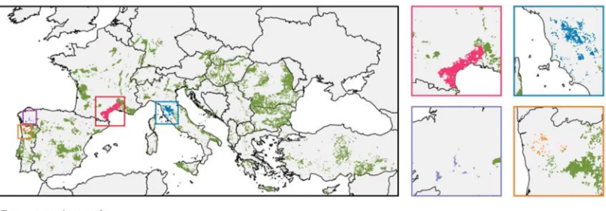
In this case study, four scenarios were defined according to the principal countries of origin of wine consumed in Québec, Canada: France (30% market share), Italy (23%), Spain (8%), and Portugal (4%) [39]. The coverage of European vineyards was obtained from the CORINE program of the European Environment Agency [35] and the QGIS v2.14.15 software was used to relate vineyard area and geopolitical information. Based on scientific literature on the environmental assessment of grapes and wine production, one wine-growing region by country was selected according to the following criteria: (1) the wine region is specified in the study, (2) the year of the inventory collection is reported, and (3) the amount of copper-based fungicide applied is reported (Figure 1). Organic vineyards were not distinguished from conventional vineyards because copper-based fungicides are applied to combat downy mildew in both farming practices [5]. Furthermore, the proportion of organic vineyards at country level is relatively low: 9% in France, 13% in Italy, 10% in Spain, and 1% in Portugal [40].

Figure 1.Location of wine regions analyzed in this case study.

The inventory of each scenario (wine-growing regions) was built with data from the literature.

In cases in which the inventory is reported by a functional unit defined as a 750-mL wine bottle,

the yield of grapes (mass of harvested grapes per surface of soil) and wine yield (volume of wine per

mass of grapes) were used to obtain an inventory per kilogram of grapes (Table 1). We acknowledge that the difference in the year of inventory collection affects the amount of copper-based fungicides applied in each region (Table 1). This is recognized as a limitation of the comparison between the selected scenarios. The year-to-year variability of inventory in viticulture is mainly driven by varying meteorological conditions. This was shown in a study analyzing 4 years of production in Galician wineries, where, for instance, the ecotoxicity impact of a wine bottle produced in 2010 was 94% higher as compared to production in 2007 [3]. Additionally, wine type and appellations are reported in Table 1 where available.

Because the aim of this case study is to assess the terrestrial ecotoxicity impact of copper-based fungicides, the agricultural field was allocated to the ecosphere. This is in line with the recommendation by the Glasgow Consensus to define the boundary between the technosphere and the ecosphere according to the goal and scope of the LCA study [41]. Regarding the inventory modelling of copper emissions, a pesticide model, such as PestLCI, was not used for two reasons: it allocates the agricultural field to the technosphere and even the viticulture-customized version of PestLCI 2.0 is not able to model copper emissions [42]. In order to avoid potential overlaps between inventory modelling and impact assessment, we assumed that the amount of copper applied is emitted 100% to agricultural soil in accordance with the approach of the widely used ecoinvent life-cycle inventory database [43].

Furthermore, this avoids underestimating the potential ecotoxic effects at the end of life of vines, which is coherent with the precautionary principle and the egalitarian perspective in LCA [44].

The impact score of each scenario was obtained according to Equation (8), where I

is the terrestrial ecotoxicity impact score (PAF·m

·day·kg

) of wine-growing region w, m

is the amount of copper emitted to soil per kg of grapes (kg Cu·kg

), and CF

is the characterization factor for copper terrestrial ecotoxicity (PAF·m

·day·kg

) of wine-growing region w at a given spatial resolution.

I

= m

· CF

(8)

3. Results and Discussion

3.1. Characterization Factors for Copper Terrestrial Ecotoxicity

CFs for copper terrestrial ecotoxicity were obtained at the spatial resolution of soil mapping units of the HWSD. CFs within 95% spatial variability are represented in Figures 2 and 3 for the method based on empirical regression models and for the method based on WHAM 6.0, respectively. The geographical variability of CFs obtained with empirical regression models is around 7.3 orders of magnitude between the lowest and highest value, with a median value of 1.88 × 10

PAF·m

·day·kg

. To put these results into perspective, Owsianiak et al. [19] found a spatial variability of 3.5 orders of magnitude with a median value of 1.4 × 10

PAF·m

·day·kg

, and Peña et al. [25] reported a spatial variability of CFs over 1.5 orders of magnitude with a mean value of 2.3 × 10

PAF·m

·day·kg

. The differences in the extent of the CFs calculated in this study and those obtained by Owsianiak et al. [19] are attributed to the soil sample size, soil properties, and the soil database used (Table S5). Moreover, in this study, FFs for a direct emission of metal in agricultural soil were integrated into the computation of CFs, whereas Owsianiak et al. [19] and Peña et al. [25]

applied FFs of metal in natural soil for an emission to continental rural air, which may explain an impact lower by around 1 order of magnitude, as all that is emitted to air does not reach the agricultural soil but rather is distributed among all the deposition compartments at the continental scale in USEtox or advected with air outside of the continental box. Most of the undefined CFs occurred in soil mapping units where the CaCO

content is greater than 0% (Figures 2 and 3 and Figure S1).

A spatial variability over 6.6 orders of magnitude was found for CFs obtained with the method based on WHAM 6.0, which is mainly caused by the geographical variability of BFs (Table S5).

Nevertheless, when considering a 95% spatial variability interval (2.5th and 97.5th percentiles),

CFs for copper terrestrial ecotoxicity span 5.5 orders of magnitude (Figure 3), with a median CF

of 1.71 × 10

PAF·m

·day·kg

. In comparison, Plouffe et al. [21] estimated zinc speciation with WHAM 6.0 and derived CFs, for which the BF was based on the true solution fraction (free ions and ions pairs). The authors found that true solution CFs for zinc terrestrial ecotoxicity span over 14.3 orders of magnitude.

CFs derived from both methods show a similar pattern with respect to soil organic matter content and pH (Figures S7 and S8). Higher values of CFs occurred where organic matter content is low, but the influence of pH was found to be less significant with respect to organic matter content. This trend is explained by the fact that soil pH has less impact on copper partitioning between the solid and aqueous phases because copper has a high affinity for organic matter [45]. The differences in the orders of magnitude of CFs derived from both methods were mainly determined by the extent of FFs (Figure S3). Regardless of the method, higher FFs resulted from higher K

values, which is explained by a lower contribution of removal processes (runoff and leaching) when the concentration of copper in the aqueous phase is lower.

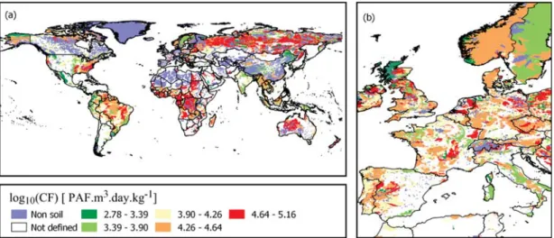
Figure 2.Regionalized characterization factors (CFs) for copper terrestrial ecotoxicity at Harmonized World Soil Database (HWSD) soil mapping unit resolution obtained with empirical regression models.

(a) Map of the world indicating the calculated CFs. (b) Zoom of European wine-growing countries.

PAF, potentially affected fraction.

Figure 3.Regionalized CFs for copper terrestrial ecotoxicity at HWSD soil mapping unit resolution obtained with WHAM 6.0. (a) Map of the world indicating the calculated CFs. (b) Zoom of European wine-growing countries.

The CFs computed in this study are in shapefile format as attributes of the soil mapping units of the HWSD. These geographical information system (GIS) data can be imported, for instance, with openLCA open-source software, which includes an implementation approach to conduct GIS-based regionalized LCA. This approach enables the LCA practitioner to define geographic regions, and openLCA then calculates the corresponding area-weighted CF according to Equation (8) for the geographical zone defined by the user [46]. However, openLCA executes spatial calculations in WGS84 projection, which can potentially bias the actual area. Alternatively, the shapefiles may be loaded in a GIS software, such as QGIS, and it is possible to set an equal area projection, such as Mollweide, to compute surfaces and derive CFs at spatial resolutions other than those presented in Sections 2.3 and 3.2. Consequently, the application of the derived CFs is not limited to this case study (Section 3.2). Besides, the LCA practitioner can establish the most appropriate proxy to aggregate CFs for the case study or use the default area weighting of openLCA. For instance, alternative proxies may be based on regionalized inventories of pollutants or on the location of the activities of the analyzed case study (e.g., mining sector). The latter proxy may be calculated by geospatial analysis, which makes it possible to correlate CFs at native resolution with a map of the analyzed economic sector.

Another potential application of the CFs derived in this study is in territorial LCA.

Nitschelm et al. [47] developed a spatialized territorial LCA (STLCA) method for territories in which the main economic activity is agriculture. This method aims to consider the spatial variability of both the inventory and the potential environmental impacts of agriculture within a territory. Territorial LCA can serve to evaluate the current situation, to analyze different scenarios, or to assess future situations [47]. The latter application could be relevant for future planning scenarios in viticulture because climate change will affect the distribution of current European wine-growing regions by 2050 [48]. Furthermore, there is a growing interest to couple Environmental Management Systems with LCA in the evaluation and management of environmental issues at the territorial level [49,50].

3.2. Characterization Factors at Different Spatial Resolutions

The global aggregated CFs for copper terrestrial ecotoxicity calculated with both methods are approximately equivalent to 3.27 × 10

PAF·m

·day·kg

. For both methods, the CF aggregated at the global scale is greater than the corresponding CF aggregated at the continental scale derived from European vineyards’ soils. The aggregated CF for European vineyards derived from the method based on WHAM 6.0 is 1.42 × 10

PAF·m

·day·kg

, and the aggregated CF obtained with empirical regressions is 2.47 × 10

PAF·m

·day·kg

. These aggregated CFs are approximately 3.8 and 3.6 orders of magnitude lower than the CF for the copper terrestrial ecotoxicity of IMPACT 2002+ (9.9 × 10

PAF·m

·day·kg

) [51], respectively. These results demonstrate the relevance of including metal speciation in the calculation of CFs for the assessment of metal terrestrial ecotoxicity.

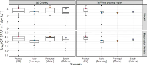
The aggregated CFs at the country and wine-growing region levels are shown in Figure 4 with their

respective spatial variability. In this figure, the width of boxes is proportional to the number of CFs of a

scenario at a given spatial resolution (country or wine-growing region). Given that life-cycle inventory

databases, such as ecoinvent, have a spatial resolution at country level, it would be appropriate to

aggregate CFs at country-level spatial resolution. However, the higher spatial variability of CF factors

at country level is approximately 2.5 orders of magnitude for the method applying empirical regression

models and 7.2 orders of magnitude for the method based on WHAM 6.0, respectively. Figure 4

shows that CFs obtained with both methods follow a similar pattern. CFs at a spatial resolution of

wine-growing regions have a lower geographical variability than CFs at country level. By applying

the empirical regression models, the higher spatial variability of CFs at the wine-growing region level

is 1.7 orders of magnitude, while that for CFs obtained with WHAM 6.0 is approximately 5.9 orders

of magnitude.

Figure 4. Site-dependent CFs for copper terrestrial ecotoxicity at the (a) country level and (b) wine-growing region level.

The aggregated CFs at the country level obtained with empirical regressions extend over 2.5 orders of magnitude for France, 1.7 for Italy, 1 for Portugal, and 2 for Spain (Figure 4), which are roughly in the range of the common uncertainty for ecotoxicity assessment (2 orders of magnitude). The aggregated CFs for France, Italy, Portugal, and Spain are in the same order of magnitude and respectively 3.51 × 10

, 1.29 × 10

, 3.47 × 10

, and 2.48 × 10

PAF·m

·day·kg

. Except for France and Portugal, these CFs are lower than the global CF (3.27 × 10

PAF·m

·day·kg

). The spatial variability of the CFs at the wine-growing region level is in the following increasing order, which is related to the surface of vineyards: Minho (36.9 km

), Galicia (59.6 km

), Languedoc-Roussillon (4470 km

), and Tuscany (447 km

). In the case of Minho (Portugal), only one soil type is present and, as a result, the CF takes a unique value of 1.13 × 10

PAF·m

·day·kg

. The spatial variability of CFs for Galicia (Spain) is negligible, with minimum and maximum values of 1.13 × 10

and 1.94 × 10

PAF·m

·day·kg

, respectively. CFs for Tuscany (Italy) and Languedoc-Roussillon (France) span over 1.7 and 1.1 orders of magnitude, respectively. However, the aggregated CF for Tuscany is lower than that for Languedoc-Roussillon (Figure 4). The aggregated CFs for Tuscany and Languedoc-Roussillon at the wine-growing region level are 1.27 × 10

and 3.69 × 10

PAF·m

·day·kg

, respectively.

When applying the method based on WHAM 6.0, CFs at the country level that correspond to

France showed higher spatial variability (approximately 7.2 orders of magnitude), while CFs for

Portugal exhibited the lowest spatial variability, around 3 orders of magnitude. CFs for Italy and

Spain span over 5.9 and 6.2 orders of magnitude, respectively (Figure 4). Aggregated CFs for France,

Italy, Portugal, and Spain are 2.04 × 10

, 1.88 × 10

, 4.16 × 10

, and 1.36 × 10

PAF·m

·day·kg

,

respectively. With the exception of Portugal, aggregated CFs at country level are lower than the

global CF (3.27 × 10

PAF·m

·day·kg

). The aggregated CF for Italy obtained by applying empirical

regression models is around 6.9 times the value calculated with WHAM 6.0, over 1.7 times for

France and Spain, and 0.8 times for Portugal. The aggregated CFs at the wine-growing region

level for Galicia, Languedoc-Roussillon, Minho, and Tuscany are 1.65 × 10

, 1.53 × 10

, 6.82 × 10

,

and 1.08 × 10

PAF·m

·day·kg

, respectively, which are lower than the global CF obtained with

WHAM 6.0 (3.27 × 10

PAF·m

·day·kg

). CFs for Tuscany show higher geographical variability,

which is around 5.9 orders of magnitude. CFs for Languedoc-Roussillon span over 3 orders of

magnitude, while the spatial variability of CFs for Galicia is around 0.5 orders of magnitude and zero

in the case of Minho.

3.3. Terrestrial Ecotoxicity Impact Score

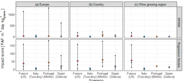
Figure 5 shows the impact score calculated for each scenario by applying CFs for copper terrestrial ecotoxicity at different spatial resolutions and calculated with empirical regression models and WHAM 6.0. Additionally, vertical lines indicate the extent of the impact score that results from applying the minimum and maximum CFs. For both methods, an increase in the spatial resolution of the CFs translates into a reduction in the geographical variability of impacts (Figure 5), following the tendency of CF spatial variability (Figure 4). Regardless of the method used to compute CFs, when using the aggregated CF for European vineyards, the rank of an impact score is determined by the amount of copper applied in each wine-growing region. This is equivalent to using a generic CF, which is a current practice in LCA. The impact score ranking therefore follows the decreasing order defined by the amount of copper applied in the wine-growing regions that were analyzed: Minho (Portugal), Languedoc-Roussillon (France), Galicia (Spain), and Tuscany (Italy) (Table 1 and Figure 5).

Nevertheless, the impact scores obtained with the global CF derived with empirical regressions are approximately 1.7 times the impact scores calculated with WHAM 6.0 (Figure 5).

When using CFs calculated with empirical regression models, the ranking of the country-level impact scores calculated with CFs is the same as the one obtained with CFs for European vineyards (Figure 5a,b, upper panel). This tendency is determined by the amount of copper-based fungicides applied in each wine-growing region, since the ranking of the aggregated CFs is the same regardless of the European vineyard or country resolution. However, the impact score ranking changes when using CFs at the wine-growing region level with respect to that obtained at the European and country resolutions. The ranking of impact scores obtained with CFs at the wine-growing region level in descending order is Languedoc-Roussillon (France), Minho (Portugal), Galicia (Spain), and Tuscany (Italy) (Figure 5c, upper panel). There is an inversion of the ranking of impact scores between Languedoc-Roussillon (France) and Minho (Portugal) because the aggregated CFs at the wine-growing region level for Minho (Portugal) is one third of the corresponding aggregated CF at country level.

Figure 5. Terrestrial ecotoxicity impact score calculated with CFs at different spatial resolutions:

(a) Europe, (b) country, and (c) wine-growing regions. Vertical lines indicate the range of impact scores obtained with the minimum and maximum CFs.

A similar pattern is obtained when applying CFs calculated with the method based on the

WHAM 6.0 model. The ranking of impact scores obtained with aggregated CFs for European

vineyards is equal to the ranking obtained when applying CFs at the country level: Portugal (Minho),

France (Languedoc-Roussillon), Spain (Galicia), and Tuscany (Italy). However, the impact score for

Minho (Portugal) and Languedoc-Roussillon (France) at the country level is 2.9 and 1.43 times the impact obtained with the aggregated CF for European vineyards, respectively. With regard to the country-level impact scores, Portugal (Minho) ranks first, France (Languedoc-Roussillon) ranks second, and Spain (Galicia) ranks third. However, these positions change when applying aggregated CFs at the wine-growing level. The impact score calculated with CFs at European vineyards is 60 and 8 times the corresponding score obtained with CFs aggregated at wine-growing regions and over 1.3 times for France and Italy.

The ranking of the impact scores of the selected scenarios is mainly determined by the amount of copper-based fungicides applied in each wine-growing region, thus demonstrating the relevance of regionalizing the inventory of agricultural systems since they are highly dependent on spatial conditions, such as climate, soil properties, and agricultural practices. For the analyzed scenarios, the higher amount of copper per kilogram of grapes is approximately 20 times the lower copper application rate (for Tuscany and Minho, respectively). However, the difference in the years of production (2007 for Tuscany and 2008 for the remaining wine-growing regions) limits the comparison and highlights the need to consider the temporal scale in the inventory of viticulture phase [3]. Even so, for the same production year, differences of more or less 50% in copper application rates are observed. Given these results, it would have been acceptable to compute the terrestrial ecotoxicity impact with a CF aggregated at the European vineyard level. However, the advantage of using finer spatial resolutions is the decrease in the uncertainty of the calculated impact score.

4. Conclusions

In this study, the two methods used to compute CFs make it possible to consider the influence of the geographical variability of soil and agricultural practices on the terrestrial ecotoxicity impact of copper-based fungicides applied in European vineyards. For both methods applied to develop regionalized CFs, an increase in the spatial resolution of CFs translated into a decrease in the spatial variability of the CFs. With the exception of the aggregated CF for Portugal (Minho) at the country level, all the aggregated CFs derived from empirical regression models are greater than the ones derived from the method based on WHAM 6.0 in a range of 0.2 to 1.2 orders of magnitude. Furthermore, CFs calculated with WHAM 6.0 exhibited greater spatial variability with respect to the CFs derived from empirical regression models. One limitation is common to both methods: the fact that CFs are only defined for non-calcareous soils because the TBLMs employed to derive EFs are not applicable to calcareous soils. Further research on how to assess the ecotoxicity of metals in calcareous soils is therefore required. Another limitation of this study is the fact that the essentiality of metal was not considered. This would require more information on the sensitivity of a broader set of terrestrial organisms and the mapping of their spatial distribution.

This study also shows the relevance of including metal speciation and bioavailability in the computation of CFs for copper terrestrial ecotoxicity since neglecting copper speciation in soil potentially overestimates the impact of copper by almost 4 orders of magnitude. Furthermore, this study illustrates the feasibility of including regionalization in both the inventory and impact assessment phases. The spatial variability of the inventory of copper emissions mainly determined the ranking of the impact scores among the wine-growing regions in the case study, highlighting the need to regionalize the inventory of agricultural systems. The regionalized CFs facilitated the computation of aggregated CFs at different spatial levels and, in all the cases, finer spatial resolutions translated into a lower uncertainty, corresponding to the spatial variability.

Supplementary Materials:The following are available online athttp://www.mdpi.com/2071-1050/10/7/2522/

s1.

Author Contributions:I.V.S. was the first author on the manuscript, carried out the main data analysis, and wrote the original draft. C.B. contributed to the research design, supervision of the project, and revision of the manuscript.

A.L. was also involved in the supervision of the project, contributed to the methodological definition, and carried

out a detailed revision of the manuscript. L.D. was the main supervisor of the project. She participated in the project conception and helped to revise the manuscript. All authors read and approved the final manuscript.

Funding:This research was funded by [Natural Sciences and Engineering Research Council of Canada] grant number [RDCPJ 451916-13] in collaboration with Hydro Quebec and the Sociétédes Alcools du Québec.

Acknowledgments:The authors would like to thank Geneviève Plouffe for her share of expertise.

Conflicts of Interest:The authors declare no conflict of interest.

References

1. Notarnicola, B.; Sala, S.; Anton, A.; McLaren, S.J.; Saouter, E.; Sonesson, U. The role of life cycle assessment in supporting sustainable agri-food systems: A review of the challenges.J. Clean. Prod.2016,140, 399–409.

[CrossRef]

2. Sala, S.; Anton, A.; McLaren, S.J.; Notarnicola, B.; Saouter, E.; Sonesson, U. In quest of reducing the environmental impacts of food production and consumption.J. Clean. Prod.2016,140, 387–398. [CrossRef]

3. Vázquez-Rowe, I.; Villanueva-Rey, P.; Moreira, M.T.; Feijoo, G. Environmental analysis of Ribeiro wine from a timeline perspective: Harvest year matters when reporting environmental impacts.J. Environ. Manag.

2012,98, 73–83. [CrossRef] [PubMed]

4. Falcone, G.; De Luca, A.; Stillitano, T.; Strano, A.; Romeo, G.; Gulisano, G. Assessment of environmental and economic impacts of vine-growing combining life cycle assessment, life cycle costing and multicriterial analysis.Sustainability2016,8, 793. [CrossRef]

5. Komárek, M.; ˇCadková, E.; Chrastný, V.; Bordas, F.; Bollinger, J.-C. Contamination of vineyard soils with fungicides: A review of environmental and toxicological aspects.Environ. Int.2010,36, 138–151. [CrossRef]

[PubMed]

6. Ruyters, S.; Salaets, P.; Oorts, K.; Smolders, E. Copper toxicity in soils under established vineyards in europe:

A survey.Sci. Total Environ.2013,443, 470–477. [CrossRef] [PubMed]

7. Bart, S.; Laurent, C.; Péry, A.R.R.; Mougin, C.; Pelosi, C. Differences in sensitivity between earthworms and enchytraeids exposed to two commercial fungicides.Ecotoxicol. Environ. Saf.2017,140, 177–184. [CrossRef]

[PubMed]

8. Fernández, D.; Voss, K.; Bundschuh, M.; Zubrod, J.P.; Schäfer, R.B. Effects of fungicides on decomposer communities and litter decomposition in vineyard streams.Sci. Total Environ.2015,533, 40–48. [CrossRef]

[PubMed]

9. Frankart, C.; Eullaffroy, P.; Vernet, G. Photosynthetic responses of lemna minor exposed to xenobiotics, copper, and their combinations.Ecotoxicol. Environ. Saf.2002,53, 439–445. [CrossRef]

10. Villanueva-Rey, P.; Vázquez-Rowe, I.; Moreira, M.T.; Feijoo, G. Comparative life cycle assessment in the wine sector: Biodynamic vs. Conventional viticulture activities in nw spain.J. Clean. Prod.2014,65, 330–341.

[CrossRef]

11. Plouffe, G.; Bulle, C.; Deschênes, L. Case study: Taking zinc speciation into account in terrestrial ecotoxicity considerably impacts life cycle assessment results.J. Clean. Prod.2015,108, 1002–1008. [CrossRef]

12. Potting, J.; Hauschild, M. Spatial differentiation in life cycle impact assessment: A decade of method development to increase the environmental realism of LCIA.Int. J. Life Cycle Assess.2006,11, 11–13.

13. Patouillard, L.; Bulle, C.; Margni, M. Ready-to-use and advanced methodologies to prioritise the regionalisation effort in LCA.Matériaux Tech.2016,104, 105. [CrossRef]

14. Mutel, C.L.; Hellweg, S. Regionalized life cycle assessment: Computational methodology and application to inventory databases.Environ. Sci. Technol.2009,43, 5797–5803. [CrossRef] [PubMed]

15. Roy, P.-O.; Azevedo, L.B.; Margni, M.; van Zelm, R.; Deschênes, L.; Huijbregts, M.A.J. Characterization factors for terrestrial acidification at the global scale: A systematic analysis of spatial variability and uncertainty.

Sci. Total Environ.2014,500–501, 270–276. [CrossRef] [PubMed]

16. USEtox. Unep/Setac Scientific Consensus Model for Characterizing Human Toxicological and Ecotoxicological Impacts of Chemical Emissions in Life Cycle Assessment. Available online:http://www.usetox.org/model/

documentation(accessed on 11 December 2017).

17. Dong, Y.; Gandhi, N.; Hauschild, M.Z. Development of comparative toxicity potentials of 14 cationic metals in freshwater.Chemosphere2014,112, 26–33. [CrossRef] [PubMed]

18. Gandhi, N.; Diamond, M.L.; van de Meent, D.; Huijbregts, M.A.J.; Peijnenburg, W.J.G.M.; Guinée, J.

New method for calculating comparative toxicity potential of cationic metals in freshwater: Application to Copper, Nickel, and Zinc.Environ. Sci. Technol.2010,44, 5195–5201. [CrossRef] [PubMed]

19. Owsianiak, M.; Rosenbaum, R.K.; Huijbregts, M.A.J.; Hauschild, M.Z. Addressing geographic variability in the comparative toxicity potential of Copper and Nickel in soils.Environ. Sci. Technol.2013,47, 3241–3250.

[CrossRef] [PubMed]

20. Plouffe, G.; Bulle, C.; Deschênes, L. Assessing the variability of the bioavailable fraction of zinc at the global scale using geochemical modeling and soil archetypes.Int. J. Life Cycle Assess.2015,20, 527–540. [CrossRef]

21. Plouffe, G.; Bulle, C.; Deschênes, L. Characterization factors for zinc terrestrial ecotoxicity including speciation.Int. J. Life Cycle Assess.2016,21, 523–535. [CrossRef]

22. Cabral Pinto, M.M.S.; Dinis, P.A.; Silva, M.M.V.G.; Ferreira da Silva, E.A. Sediment generation on a volcanic island with arid tropical climate: A perspective based on geochemical maps of topsoils and stream sediments from Santiago Island, cape verde.Appl. Geochem.2016,75, 114–124. [CrossRef]

23. Cabral Pinto, M.M.S.; Silva, M.M.V.G.; Ferreira da Silva, E.A.; Dinis, P.A.; Rocha, F. Transfer processes of potentially toxic elements (pte) from rocks to soils and the origin of pte in soils: A case study on the island of santiago (cape verde).J. Geochem. Explor.2017,183, 140–151. [CrossRef]

24. Aziz, L.; Deschênes, L.; Karim, R.-A.; Patouillard, L.; Bulle, C. Including metal atmospheric fate and speciation in soils for terrestrial ecotoxicity in life cycle impact assessment. Int. J. Life Cycle Assess.2018.

[CrossRef]

25. Peña, N.; Antón, A.; Kamilaris, A.; Fantke, P. Modeling ecotoxicity impacts in vineyard production:

Addressing spatial differentiation for copper fungicides.Sci. Total Environ.2017,616, 796–804. [CrossRef]

[PubMed]

26. Diamond, M.; Gandhi, N.; Adams, W.; Atherton, J.; Bhavsar, S.; Bulle, C.; Campbell, P.C.; Dubreuil, A.;

Fairbrother, A.; Farley, K.; et al. The clearwater consensus: The estimation of metal hazard in fresh water.

Int. J. Life Cycle Assess.2010,15, 143–147. [CrossRef]

27. Groenenberg, J.E.; Römkens, P.F.A.M.; Comans, R.N.J.; Luster, J.; Pampura, T.; Shotbolt, L.; Tipping, E.;

De Vries, W. Transfer functions for solid-solution partitioning of Cadmium, Copper, Nickel, Lead and Zinc in soils: Derivation of relationships for free metal ion activities and validation with independent data.Eur. J.

Soil Sci.2010,61, 58–73. [CrossRef]

28. FAO/IIASA/ISRIC/ISS-CAS/JRC.Harmonized World Soil Database (Version 1.2); FAO/IIASA, Ed.; FAO:

Rome, Italy; IIASA: Laxenburg, Austria, 2012.

29. Henderson, A.D.; Hauschild, M.Z.; Meent, D.; Huijbregts, M.A.J.; Larsen, H.F.; Margni, M.; McKone, T.E.;

Payet, J.; Rosenbaum, R.K.; Jolliet, O. USEtox fate and ecotoxicity factors for comparative assessment of toxic emissions in life cycle analysis: Sensitivity to key chemical properties.Int. J. Life Cycle Assess.2011,16, 701–709. [CrossRef]

30. Kabata-Pendias, A.; Mukherjee, A.B.Trace Elements from Soil to Human; Springer Science & Business Media:

Berlin, Germany, 2007.

31. Römkens, P.F.A.M.; Groenenberg, J.E.; Bonten, L.T.C.; Vries, W.D.; Bril, J.Derivation of Partition Relationships to Calculate Cd, Cu, Ni, Pb, Zn Solubility and Activity in Soil Solutions; Alterra: Wageningen, The Netherlands, 2004; p. 75.

32. Rosenbaum, R.; Bachmann, T.; Gold, L.; Huijbregts, M.J.; Jolliet, O.; Juraske, R.; Koehler, A.; Larsen, H.;

MacLeod, M.; Margni, M.; et al. USEtox—The UNEP-SETAC toxicity model: Recommended characterisation factors for human toxicity and freshwater ecotoxicity in life cycle impact assessment.Int. J. Life Cycle Assess.

2008,13, 532–546. [CrossRef]

33. Tromson, C.; Bulle, C.; Deschênes, L. Including the spatial variability of metal speciation in the effect factor in life cycle impact assessment: Limits of the equilibrium partitioning method. Sci. Total Environ. 2017, 581–582, 117–125. [CrossRef] [PubMed]

34. Thakali, S.; Allen, H.E.; Di Toro, D.M.; Ponizovsky, A.A.; Rooney, C.P.; Zhao, F.-J.; McGrath, S.P.; Criel, P.;

Van Eeckhout, H.; Janssen, C.R.; et al. Terrestrial biotic ligand model. 2. Application to Ni and Cu toxicities to plants, invertebrates, and microbes in soil.Environ. Sci. Technol.2006,40, 7094–7100. [CrossRef] [PubMed]

35. European Environment Agency (EEA).Corine Land Cover 2000 (clc200)-221 Vineyards; Agency, E.E., Ed.;

EEA: Copenhagen, Denmark, 2017.

36. Neto, B.; Dias, A.; Machado, M. Life cycle assessment of the supply chain of a portuguese wine:

From viticulture to distribution.Int. J. Life Cycle Assess.2013,18, 590–602. [CrossRef]

37. Vázquez-Rowe, I.; Rugani, B.; Benetto, E. Tapping carbon footprint variations in the european wine sector.

J. Clean. Prod.2013,43, 146–155. [CrossRef]

38. Bellon-Maurel, V.; Peters, G.M.; Clermidy, S.; Frizarin, G.; Sinfort, C.; Ojeda, H.; Roux, P.; Short, M.D.

Streamlining life cycle inventory data generation in agriculture using traceability data and information and communication technologies-part ii: Application to viticulture.J. Clean. Prod.2015,87, 119–129. [CrossRef]

39. SAQ. Annual Report 2015-Discovery Destination. Available online:http://s7d9.scene7.com/is/content/

SAQ/rapport-annuel-2015-en(accessed on 5 June 2017).

40. Eurostat. Area of Vineyards by Size Class of the Wine-Grower Holding, 2015. Available online:

http://ec.europa.eu/eurostat/statistics-explained/index.php?title=File:Area_of_vineyards_by_size_

class_of_the_wine-grower_holding,_2015.png(accessed on 29 June 2018).

41. Rosenbaum, R.; Anton, A.; Bengoa, X.; Bjørn, A.; Brain, R.; Bulle, C.; Cosme, N.; Dijkman, T.; Fantke, P.;

Felix, M.; et al. The glasgow consensus on the delineation between pesticide emission inventory and impact assessment for LCA.Int. J. Life Cycle Assess.2015,20, 765–776. [CrossRef]

42. Renaud-Gentié, C.; Dijkman, T.; Bjørn, A.; Birkved, M. Pesticide emission modelling and freshwater ecotoxicity assessment for grapevine LCA: Adaptation of pestlci 2.0 to viticulture.Int. J. Life Cycle Assess.

2015. [CrossRef]

43. Nemecek, T.; Kägi, T.; Blaser, S. Life cycle inventories of agricultural production systems.Final Rep. Ecoinvent 2007,2, 15.

44. Hellweg, S.; Hofstetter, T.B.; Hungerbuhler, K. Discounting and the environment should current impacts be weighted differently than impacts harming future generations?Int. J. Life Cycle Assess.2003,8, 8–18.

45. Ivezi´c, V.; Almås, Å.R.; Singh, B.R. Predicting the solubility of Cd, Cu, Pb and Zn in uncontaminated croatian soils under different land uses by applying established regression models. Geoderma2012,170, 89–95. [CrossRef]

46. Rodríguez, C.; Ciroth, A.; Srocka, M. The importance of regionalized LCIA in agricultural LCA—New software implementation and case study. In Proceedings of the 9th International Conference Life Cycle Assess Agri-Food Sector, San Francisco, CA, USA, 8–10 October 2014; pp. 1120–1128.

47. Nitschelm, L.; Aubin, J.; Corson, M.S.; Viaud, V.; Walter, C. Spatial differentiation in life cycle assessment LCA applied to an agricultural territory: Current practices and method development.J. Clean. Prod.2016, 112, 2472–2484. [CrossRef]

48. Moriondo, M.; Jones, G.V.; Bois, B.; Dibari, C.; Ferrise, R.; Trombi, G.; Bindi, M. Projected shifts of wine regions in response to climate change.Clim. Chang.2013,119, 825–839. [CrossRef]

49. Loiseau, E.; Aissani, L.; Le Féon, S.; Laurent, F.; Cerceau, J.; Sala, S.; Roux, P. Territorial life cycle assessment (LCA): What exactly is it about? A proposal towards using a common terminology and a research agenda.

J. Clean. Prod.2018,176, 474–485. [CrossRef]

50. Mazzi, A.; Toniolo, S.; Catto, S.; De Lorenzi, V.; Scipioni, A. The combination of an environmental management system and life cycle assessment at the territorial level.Environ. Impact Assess. Rev.2017,63, 59–71. [CrossRef]

51. Jolliet, O.; Margni, M.; Charles, R.; Humbert, S.; Payet, J.; Rebitzer, G.; Rosenbaum, R. Impact 2002+: A new life cycle impact assessment methodology.Int. J. Life Cycle Assess.2003,8, 324–330. [CrossRef]

© 2018 by the authors. Licensee MDPI, Basel, Switzerland. This article is an open access article distributed under the terms and conditions of the Creative Commons Attribution (CC BY) license (http://creativecommons.org/licenses/by/4.0/).