HAL Id: hal-02414377
https://hal.archives-ouvertes.fr/hal-02414377
Submitted on 16 Sep 2020
HAL is a multi-disciplinary open access
archive for the deposit and dissemination of
sci-entific research documents, whether they are
pub-lished or not. The documents may come from
teaching and research institutions in France or
abroad, or from public or private research centers.
L’archive ouverte pluridisciplinaire HAL, est
destinée au dépôt et à la diffusion de documents
scientifiques de niveau recherche, publiés ou non,
émanant des établissements d’enseignement et de
recherche français ou étrangers, des laboratoires
publics ou privés.
atmospheric inverse modelling approach using a regional
measurement network
Emily White, Matthew Rigby, Mark Lunt, T. Luke Smallman, Edward
Comyn-Platt, Alistair Manning, Anita Ganesan, Simon O ’ Doherty, Ann
Stavert, Kieran Stanley, et al.
To cite this version:
Emily White, Matthew Rigby, Mark Lunt, T. Luke Smallman, Edward Comyn-Platt, et al..
Quan-tifying the UK’s carbon dioxide flux: an atmospheric inverse modelling approach using a regional
measurement network. Atmospheric Chemistry and Physics, European Geosciences Union, 2019, 19
(7), pp.4345-4365. �10.5194/acp-19-4345-2019�. �hal-02414377�
https://doi.org/10.5194/acp-19-4345-2019 © Author(s) 2019. This work is distributed under the Creative Commons Attribution 4.0 License.
Quantifying the UK’s carbon dioxide flux: an atmospheric inverse
modelling approach using a regional measurement network
Emily D. White1, Matthew Rigby1, Mark F. Lunt1,2, T. Luke Smallman2,3, Edward Comyn-Platt4,
Alistair J. Manning5, Anita L. Ganesan6, Simon O’Doherty1, Ann R. Stavert1,7, Kieran Stanley1, Mathew Williams2,3, Peter Levy8, Michel Ramonet9, Grant L. Forster10,11, Andrew C. Manning10, and Paul I. Palmer2
1School of Chemistry, University of Bristol, Bristol, BS8 1TS, UK
2School of GeoSciences, University of Edinburgh, Edinburgh, EH9 3FF, UK 3National Centre for Earth Observation, Edinburgh, EH9 3FF, UK
4Centre for Ecology and Hydrology, Wallingford, OX10 8BB, UK 5Hadley Centre, Met. Office, Exeter, EX1 3PB, UK
6School of Geographical Sciences, University of Bristol, Bristol, BS8 1SS, UK
7Climate Science Centre, CSIRO Oceans and Atmosphere, Aspendale, VIC 3195, Australia 8Centre for Ecology and Hydrology (Edinburgh Research Station), Penicuik, E26 0QB, UK
9Laboratoire des Sciences du Climat et de l’Environnement, CEA-CNRS-UVSQ, Gif-sur-Yvette, 91198, France 10Centre for Ocean and Atmospheric Sciences, School of Environmental Sciences,
University of East Anglia, Norwich, NR4 7TJ, UK
11National Centre for Atmospheric Science, School of Environmental Sciences,
University of East Anglia, Norwich, NR4 7TJ, UK
Correspondence: Emily D. White ([email protected]) and Matthew Rigby ([email protected]) Received: 9 August 2018 – Discussion started: 21 September 2018
Revised: 14 February 2019 – Accepted: 1 March 2019 – Published: 4 April 2019
Abstract. We present a method to derive atmospheric-observation-based estimates of carbon dioxide (CO2) fluxes
at the national scale, demonstrated using data from a net-work of surface tall-tower sites across the UK and Ireland over the period 2013–2014. The inversion is carried out us-ing simulations from a Lagrangian chemical transport model and an innovative hierarchical Bayesian Markov chain Monte Carlo (MCMC) framework, which addresses some of the tra-ditional problems faced by inverse modelling studies, such as subjectivity in the specification of model and prior uncer-tainties. Biospheric fluxes related to gross primary produc-tivity and terrestrial ecosystem respiration are solved sepa-rately in the inversion and then combined a posteriori to de-termine net ecosystem exchange of CO2. Two different
mod-els, Data Assimilation Linked Ecosystem Carbon (DALEC) and Joint UK Land Environment Simulator (JULES), pro-vide prior estimates for these fluxes. We carry out separate inversions to assess the impact of these different priors on the posterior flux estimates and evaluate the differences
be-tween the prior and posterior estimates in terms of missing model components. The Numerical Atmospheric dispersion Modelling Environment (NAME) is used to relate fluxes to the measurements taken across the regional network. Poste-rior CO2estimates from the two inversions agree within
es-timated uncertainties, despite large differences in the prior fluxes from the different models. With our method, averag-ing results from 2013 and 2014, we find a total annual net biospheric flux for the UK of 8 ± 79 Tg CO2yr−1(DALEC
prior) and 64 ± 85 Tg CO2yr−1 (JULES prior), where
neg-ative values represent an uptake of CO2. These biospheric
CO2estimates show that annual UK biospheric sources and
sinks are roughly in balance. These annual mean estimates consistently indicate a greater net release of CO2 than the
prior estimates, which show much more pronounced uptake in summer months.
1 Introduction
There are significant uncertainties in the magnitude and spatiotemporal distribution of global carbon dioxide (CO2)
fluxes to and from the atmosphere, particularly those due to terrestrial ecosystems (Le Quéré et al., 2018). Reliable methods for quantifying carbon budgets at policy-relevant scales (i.e. national or subnational) will be important to ac-curately and transparently evaluate each country’s progress towards achieving their Nationally Determined Contribu-tions (NDCs) made following the Paris Agreement (UN-FCCC, 2015).
Regional terrestrial carbon fluxes can be estimated using a range of observational, computational and inventory-based methods. These include bottom-up approaches such as the upscaling of direct flux measurements made using eddy co-variance or chamber systems (Baldocchi and Wilson, 2001) and models of atmosphere–biosphere CO2 exchange. Flux
measurements are important for understanding the small-scale processes responsible for carbon fluxes. However, they are relatively localised estimates (metres to hectares), which are challenging to scale up to national levels. Biosphere mod-els and land surface modmod-els can be used to estimate carbon fluxes using coupled representations of biogeophysical and biogeochemical processes, driven by observations of meteo-rology and ecosystem parameters (Potter, 1999; Clark et al., 2011; Bloom et al., 2016). Such models describe processes to varying degrees of complexity, with poorly described er-rors, and are driven by observational data at differing tem-poral and spatial resolutions; hence predictions of biogenic greenhouse gas (GHG) fluxes have poorly quantified biases and can vary significantly between models (Todd-Brown et al., 2013; Atkin et al., 2015).
Atmospheric inverse modelling is a top-down approach that provides an alternative to the bottom-up approaches. In-versions have been used to indirectly estimate country-scale (e.g. Matross et al., 2006; Schuh et al., 2010; Meesters et al., 2012) and continental (e.g. Gerbig et al., 2003; Peters et al., 2010; Rivier et al., 2010) biospheric CO2budgets using
atmospheric mole fraction observations, where the contribu-tion of anthropogenic fluxes to the observacontribu-tions has been re-moved. In this approach, a model of atmospheric transport relates spatiotemporally resolved surface fluxes of biospheric CO2 to atmospheric measurements of CO2mole fractions.
Biospheric fluxes derived from bottom-up approaches are often used as prior estimates in the inversion. Since atmo-spheric observations are sensitive to fluxes spanning tens to hundreds of kilometres (Gerbig et al., 2009), inverse methods are a valuable tool for examining national fluxes and evalu-ating estimates of surface exchange of CO2at larger spatial
scales. However, errors in atmospheric transport, unknown uncertainties related to the prior fluxes and issues surround-ing the underdetermined nature of the problem are all limita-tions of this approach.
The United Kingdom (UK) government has set legally binding targets to curb GHG emissions in an attempt to prevent dangerous levels of climate change. The Climate Change Act 2008 (UK government, 2008) commits the UK to 80 % cuts in GHG emissions, from 1990 levels, by 2050. To support this legislation, a continuous and automated mea-surement network has been established (Stanley et al., 2018; Stavert et al., 2018) with the goal of providing estimates of GHG emissions using methods that are complementary to those used to compile the UK’s bottom-up emissions in-ventory, reported annually to the United Nations Frame-work Convention on Climate Change (UNFCCC). Previ-ous studies have used data from the UK Deriving Emis-sions related to Climate Change (UK-DECC) network to in-fer emissions of methane, nitrous oxide and HFC-134a from the UK (Manning et al., 2011; Ganesan et al., 2015; Say et al., 2016). These studies found varying levels of agree-ment with bottom-up inventory methods, where estimates of GHG emissions are made using reported statistics from vari-ous sectors (e.g. road transport, power generation). Here we use the DECC network and two additional sites from the Greenhouse gAs Uk and Global Emissions (GAUGE) pro-gramme (Palmer et al., 2018) to estimate biospheric fluxes of CO2. Whilst anthropogenic emissions, which are the remit of
the UK inventory, are not estimated in this study, these bio-spheric estimates represent the first step towards a framework for estimating the complete UK CO2budget.
Atmospheric inverse modelling of GHGs using Bayesian methods presents some known challenges. Robust uncer-tainty quantification in Bayesian frameworks can be difficult as they require that uncertainties in the prior flux estimate, and uncertainties in the atmospheric transport model’s ability to simulate the data, are well characterised. In practice, this is rarely the case because, for example, uncertainties related to the atmospheric transport model are poorly understood and uncertainties related to biospheric flux estimates from models are largely unknown. Various studies have investi-gated the use of data-driven uncertainty estimation (Micha-lak, 2004; Berchet et al., 2013; Ganesan et al., 2014; Koun-touris et al., 2018b). Inversions are also known to suffer from aggregation errors. One type of aggregation error arises from the way in which areas of the flux domain are grouped to-gether to decrease the number of unknowns, because usually there are not sufficient data to solve for fluxes in each model grid cell (Kaminski et al., 2001). Furthermore, for reasons of mathematical and computational convenience, Gaussian probability density functions (PDFs) are commonly used to describe prior knowledge (e.g. Miller et al., 2014). However, Gaussian assumptions can lead to unphysical solutions in the case of atmospheric GHG emissions or uptake processes, as they permit both positive and negative solutions.
CO2 presents further complications over other GHGs in
that atmosphere–biosphere CO2exchange has a diurnal flux
cycle that is significantly larger than the net flux and has strong, spatially varying surface sources and sinks. Gerbig et
al. (2003) was one of the first to develop an analysis frame-work for regional-scale CO2flux inversions. The study sets
out the need to explicitly simulate the diurnal cycle of bio-spheric fluxes and highlights the importance of high spa-tial and temporal resolution data when addressing the unique problems of representation and aggregation errors caused by the highly varying nature of CO2 fluxes in both space and
time. Inverse modelling studies of CO2 flux typically
as-sume that anthropogenic fluxes are “fixed” in the inversion (e.g. Meesters et al., 2012; Kountouris et al., 2018a). This is based on the assumption that uncertainties in anthropogenic fluxes are low compared to those of the biospheric fluxes. However, it has been suggested that this may not necessarily be the case (Peylin et al., 2011).
Here we outline a framework for evaluating the net bio-spheric CO2exchange (net ecosystem exchange, NEE) from
a small- to medium-sized country (the UK covers an area of around 250 000 km2) using the high-resolution regional, La-grangian transport model, the Numerical Atmospheric dis-persion Modelling Environment (NAME, Jones et al., 2006). To address many of the problems outlined above, we use an adapted form of a hierarchical Bayesian, trans-dimensional Markov chain Monte Carlo (MCMC) inversion (Rigby et al., 2011; Ganesan et al., 2014; Lunt et al., 2016). In the hierarchical Bayesian framework presented in Ganesan et al. (2014), “hyperparameters” that define the prior flux and model–data “mismatch” uncertainty PDFs are included in the inversion, which is solved using a Metropolis–Hastings MCMC algorithm (e.g. Rigby et al., 2011). This hierarchical approach has been shown to lead to more robust posterior uncertainty quantification in Bayesian frameworks where prior uncertainties are not well characterised (Ganesan et al., 2014). Lunt et al. (2016) built on this method, developing a “trans-dimensional” framework that accounted for the uncer-tainty in the definition of basis functions (the way in which flux grid cells are aggregated) and allowed this to propagate through to the posterior estimate.
Gross primary productivity (GPP) and terrestrial ecosys-tem respiration (TER) estimates from the Joint UK Land En-vironment Simulator (JULES) and Data Assimilation Linked Ecosystem Carbon (DALEC) models are used as prior flux constraints. JULES is a state-of-the-art physically based, process-driven model that estimates the energy, water and carbon fluxes at the land–atmosphere boundary and uses a variety of observation-derived products describing physical parameters as inputs (Best et al., 2011; Clark et al., 2011). DALEC, on the other hand, is a simplified terrestrial C-cycle model which is calibrated independently at each location re-trieving both process parameters and initial conditions using the carbon data model framework (CARDAMOM) model– data fusion system. CARDAMOM ingests satellite-based re-motely sensed estimates of the state of terrestrial ecosystems (Bloom and Williams, 2015; Bloom et al., 2016; Smallman et al., 2017).
Below, we first describe our approach for modelling bio-spheric CO2 fluxes, including several novel aspects
com-pared to previous work in this area. We then investigate the impact of using two different models that simulate biospheric fluxes (JULES and DALEC) within our proposed inverse framework and discuss the discrepancies between the prior and posterior flux estimates.
2 Method
The main components of a regional atmospheric inverse modelling framework are the atmospheric CO2mole fraction
data themselves, a model of atmospheric transport including a set of boundary conditions at the edge of the regional do-main and some initial information or “first guess” of regional CO2fluxes. These components are combined in an inversion
set-up with a mechanism for dealing with uncertainties in the inputs. To make the problem computationally manage-able, the regional domain is often decomposed into a number of basis functions, describing a spatial grouping of grid cells within which fluxes are scaled up or down. The selection of these basis functions constitutes a further key element of the atmospheric inverse problem.
2.1 Site location and measurements
This study focuses on the years 2013 and 2014. During this period, atmospheric CO2mole fractions were continuously
measured at six sites across the UK and Republic of Ireland (see Table 1 for site information and Fig. 1 for the location of the sites). Four of these sites originally formed the UK-DECC network and are described in Stanley et al. (2018), whilst two were developed under the GAUGE programme and are described in Stavert et al. (2018). The site at Mace Head, Republic of Ireland, is a coastal, 10 m a.g.l. (above ground level), station situated primarily to measure con-centrations of background air arriving at the site from the Atlantic Ocean. The Laboratoire des Sciences du Climat et de l’Environnement (LSCE) is responsible for making CO2 measurements at this site from a 23 m a.g.l. inlet (see
Vardag et al., 2014, for a full site description). All of the UK sites are tall-tower stations (with inlets ranging from 42 to 248 m a.g.l.), designed to measure elevated GHG mole fractions as air is transported over the surface in the UK and Europe.
Continuous CO2measurements are made at all stations
us-ing cavity rus-ing-down spectrometers (CRDS: Picarro G2301 or G2401). CRDS data are corrected for daily linear instru-mental drift using standard gases and for instruinstru-mental non-linearity using calibration gases, spanning a range of above and below ambient mole fractions, on a monthly basis (Stan-ley et al., 2018). Calibration and standard gases are of nat-ural composition and calibrated at the GasLab, Max Planck Institute for Biogeochemistry, Jena, or the World Calibration
Figure 1. Mean annual NAME footprint for 2014, for each of the six sites. MHD: Mace Head; RGL: Ridge Hill; HFD: Heathfield; TAC: Tacolneston; BSD: Bilsdale; TTA: Angus. WAO shows the location of the Weybourne Atmospheric Observatory, where data have been used to validate the results but have not been included in the inversion (the mean footprint from this station is not plotted).
Centre for CO2at Empa, linking them to the World
Meteo-rological Organisation (WMO) X2007 scale (Stanley et al., 2018; Stavert et al., 2018). At sites with multiple inlets, mea-surements are taken for the same length of time at each inlet, each hour. This means that measurements at each height at Bilsdale and Tacolneston (with three inlets) are taken contin-uously for roughly 20 min every hour, and at Heathfield and Ridge Hill (with two inlets) measurements are taken contin-uously for roughly 30 min at each inlet every hour. For the purposes of the inverse modelling carried out in this study, the continuous CRDS data are used from the highest inlets and averaged to a 2 h time resolution. Further information about the instruments, measurement protocol and uncertainty estimates can be found in Stanley et al. (2018) and Stavert et al. (2018).
2.2 Atmospheric transport model
In this work we use a Lagrangian particle dispersion model (LPDM), NAME, which tracks thousands of parti-cles back in time from observation locations. The model de-termines the locations where air masses interacted with the surface and therefore where surface CO2sources and sinks
could contribute to a CO2concentration measurement. The
model provides a gridded sensitivity of each mole fraction observation to the potential flux from each grid cell and this is often referred to as the “footprint” of a particular observa-tion (for further details, see e.g. Manning et al., 2011).
At each 2-hourly measurement time step, the model re-leases 20 000 particles, which are tracked back in time for 30 days, so that by the end of this period the majority of particles will have left the model domain (Fig. S1 in the
Table 1. Measurement site information. The location of sites is also shown in Fig. 1.∗Weybourne data were used for validation of the results only and were not included in the inversions. LSCE – Lab-oratoire des Sciences du Climat et de l’Environnement; DECC – Deriving Emissions related to Climate Change; GAUGE – Green-house gAs Uk and Global Emissions; UEA – University of East Anglia.
Site Site Location Inlet Network
code height
(m a.g.l.) Mace Head MHD 53.327◦N, 9.904◦W 24 LSCE Ridge Hill RGL 51.998◦N, 2.540◦W 90 DECC Tacolneston TAC 52.518◦N, 1.139◦E 185 DECC Heathfield HFD 50.977◦N, 0.231◦E 100 GAUGE Bilsdale BSD 54.359◦N, 1.150◦W 248 GAUGE Angus TTA 56.555◦N, 2.986◦W 222 DECC Weybourne∗ WAO 52.950◦N, 1.122◦E 10 UEA
Supplement). Since most CO2flux to the atmosphere occurs
at the surface, we record the instances where the particles are in the lowest 40m of the atmosphere and assume that this represents the sensitivity of observed mole fractions to surface fluxes in the inversion domain. The domain used to calculate atmospheric transport covers most of Europe, the east coast of North and Central America, and North Africa (10.729–79.057◦N and 97.9◦W–39.38◦E). The spatial reso-lution of the meteorological analysis dataset used to drive the model, from the Met Office Unified Model (Cullen, 1993), was 0.233◦by 0.352◦(roughly 25 km by 25 km over the UK). In many previous inverse modelling studies using LPDMs (e.g. Manning et al., 2011; Thompson and Stohl, 2014; Steinkamp et al., 2017) the footprint is assumed to be equal to the integrated air history over the duration of the simula-tion (e.g. 30 days, as in Fig. 1). Based on the assumpsimula-tion that fluxes have not changed substantially during the 30-day pe-riod, the integrated footprint can be multiplied by the prior flux and summed over all the grid cells in the domain to cre-ate a time series of modelled mole fractions at each mea-surement site. However, many CO2inverse modelling
stud-ies using other LPDMs have disaggregated footprints back in time, capturing changes in surface sensitivity on timescales shorter than the duration of the simulation, thereby attempt-ing to account for diurnal variation in CO2fluxes (Denning
et al., 1996; Gerbig et al., 2003; Gourdji et al., 2010). Thus far, a disaggregation such as this has not been used in NAME simulations, so we describe our method here.
In our simulations, we determined the footprint for 2-hourly average periods back in time for the first 24 h before the observation and then replaced the first 24 h of integrated sensitivities with these time-disaggregated footprints. Mole fractions were simulated by multiplying these footprints by biospheric flux estimates for the corresponding time, so that the variability in the source or sink of CO2was represented
which yields the modelled mole fraction, yt, for one 2-hourly
measurement time step, t , at one measurement site.
yt= 12 X i=0 n X j =0 fpt −i,j×qt −i,j+ n X j =0 fpremainder j×qmonthj (1)
Here i denotes the number of 2 h periods back in time be-fore the particle release at time t ; j represents the grid cell where n is the maximum number of grid cells; fpt −i,j is one
grid cell of the two-dimensional time-disaggregated footprint for that time; qt −i,j is one grid cell of the two-dimensional,
2-hourly flux field corresponding to the time the particles were interacting with the surface; fpremainder is the
remain-ing 29-day footprint; and qmonthis the monthly average flux.
The choice of 24 h disaggregation balanced considerations of computational efficiency and simulation accuracy. For cer-tain months and sites we carried out a set of tests to determine how sensitive our simulated mole fractions and inversion re-sults were when footprints were disaggregated for the first 12 or 72 h prior to each measurement (Fig. S2; Table S1 in the Supplement). Assuming that the 72 h simulations were the most accurate, we found little degradation in performance by using only 48 or 24 h disaggregation, when compared to the other uncertainties in the system (e.g. differences between fluxes derived using the 24, 48 and 72 h simulations were smaller than the 90 % confidence interval). However, when only 12 h was used (or fully integrated footprints), the mod-elled diurnal cycle was out of phase with the observations. 2.2.1 Data selection and model uncertainty
LPDMs are known to perform poorly under certain me-teorological conditions. In particular, it is often assumed that model–data mismatch should be smallest during periods when the boundary layer is relatively well mixed. A com-mon approach is to only include daytime data in the inversion (e.g. Meesters et al., 2012; Steinkamp et al., 2017; Koun-touris et al., 2018a) or separate morning and afternoon aver-ages (e.g. Matross et al., 2006). To make use of as much high-frequency-measurement information as possible, we use a filter based on two metrics to remove times of high atmo-spheric stability and/or stagnant conditions. The first metric is based on calculating the ratio of the NAME footprint mag-nitude in the 25 grid boxes in the immediate vicinity of the measurement station to the total for all of the grid boxes in the domain. A high ratio indicates times when a significant fraction of air influencing the observation point originates from very local sources, which may not be resolved by the model (Lunt et al., 2016). The second metric is based on the modelled lapse rate at each site, which is a measure of at-mospheric stability. A high lapse rate suggests very stable conditions, which would be conducive for significant local influence. Thresholds for each of these criteria were chosen to preserve as much data as possible, whilst retaining only points that the model was (somewhat subjectively) found to
resolve well. In practice, the filter retained many more day-time than night-day-time points (see Fig. S3 for an analysis of the data removed in 2014) and inversion results were mostly similar to when only daytime data were used; however, dif-ferences were seen in some months when stagnant conditions occurred for several daytime periods (Fig. S4).
Model uncertainty (or model–data mismatch) has a mea-surement uncertainty component and a component that takes into account the ability of the model to represent real at-mospheric conditions. The measurement uncertainty was as-sumed to be equal to the standard deviation of the measure-ments over the 2 h period to give an estimate of measurement repeatability and a measure of the sub-model-timescale vari-ability in the observations. The 2-hourly measurement un-certainty was then averaged over the month to ensure that measurements of high concentrations were not de-weighted, as they are more likely to have greater variability and there-fore a larger standard deviation. Monthly average measure-ment uncertainty is around 0.9 ppm. The measuremeasure-ment un-certainty is combined with a range of prior values for model uncertainty (as this is a poorly constrained quantity), and together the model–measurement uncertainty is one of the hyper-parameters solved in the inversion (further explained in Sect. 2.4.1).
2.2.2 Boundary conditions
The footprints from the LPDM only take into considera-tion the influence on the observaconsidera-tions of sources intercepted within the model domain. Therefore, an estimate of the mole fraction at the boundary must be made and incorporated into the simulated mole fractions. To estimate spatial and temporal gradients in these boundary conditions we use the global Eulerian Model for OZone And Related chemical Tracers (MOZART, Emmons et al., 2010). The model was run using GEOS-5 meteorology (Rienecker et al., 2011) and global biospheric fluxes from the NASA-CASA biosphere model (Potter, 1999), global ocean fluxes from Takahashi et al. (2009) and global anthropogenic fluxes from the Emis-sion Database for Global Atmospheric Research (EDGAR, EC-JRC/PBL, 2011). When particles leave the NAME model domain, we record the time and location of the exit point. We then use MOZART to find the concentration of CO2at
these locations to serve as prior boundary conditions. The global MOZART initial mole fraction field for January 2014 was scaled before commencing the 2014 MOZART run to match the surface South Pole value to the mean NOAA January 2014 flask value (Dlugokencky et al., 2018). This scaling factor was also applied to any pre-January 2014 MOZART output to prevent any discontinuities in the bound-ary mole fraction fields. The mole fraction at each domain edge (N, E, S, W) is then scaled up or down during the inver-sion to account for uncertainties in the MOZART boundary conditions (Lunt et al., 2016). A sensitivity test where 1 ppm is added or taken away from the mole fractions at the domain
Table 2. Specifications for different prior and fixed fluxes.
Spatial resolution Temporal resolution Biogenic fluxes
JULES 0.25◦×0.25◦ 2-hourly DALEC 25 km × 25 km (1◦×1◦outside the UK) 2-hourly Anthropogenic fluxes
NAEI (UK) 1 km × 1 km 2-hourly
EDGAR (outside UK) 0.1◦×0.1◦ Yearly (using 2010) Ocean fluxes 4◦×5◦ Monthly (climatology)
Figure 2. Prior UK fluxes in 2014. (a–c) Comparison of JULES (blue) and DALEC (orange) monthly fluxes and minimum and maximum daily values for TER, GPP and NEE respectively. (d) Monthly anthropogenic fluxes and minimum and maximum daily values from the NAEI inventory within the UK. (e) Monthly coastal ocean net fluxes from the Takahashi et al. (2009) ocean CO2flux product.
edges indicates that in June a ±1 ppm change translates to a 1 %–3 % change in the inversion result and in December a ±1 ppm change translates to a 7 %–11 % change in the inver-sion result. These changes are substantially smaller than the posterior uncertainty.
2.3 Prior information
In this work, we used model analyses to provide prior infor-mation about biospheric fluxes. Two models (DALEC and JULES) were used to assess how much influence the choice of biospheric prior has on the outcome of the inversion. The NAME model was used to simulate the contribution of an-thropogenic and oceanic fluxes to the data, and this contri-bution was removed from the observations prior to the inver-sion. The fluxes used for this calculation are described below.
The spatial and temporal resolution of the prior information and fixed fluxes are summarised in Table 2 and emissions from each source over the UK are shown in Fig. 2.
In a synthetic data study in which biospheric CO2 was
inferred, Tolk et al. (2011) found that separately solving for positive fluxes (autotrophic and heterotrophic respiration combined, TER) and negative fluxes (GPP) in atmospheric inversions provided a better fit to the atmospheric mole frac-tion data than inversions that scaled NEE only. Equafrac-tion (2) describes the relationship between these three variables:
NEE = TER − GPP. (2)
This separation has been applied in various studies demon-strating model set-ups with synthetic data, for example geostatistical approaches (Göckede et al., 2010), ensemble Kalman filter methods (Zupanski et al., 2007; Lokupitiya et
al., 2008) and Bayesian methods (Schuh et al., 2009). How-ever, this separation is not routinely used in CO2inversions,
as there are only a limited number of real data studies where it has been implemented (e.g. Gerbig et al., 2003; Matross et al., 2006; Schuh et al., 2010; Meesters et al., 2012).
In this inversion, we separately solved for TER and GPP and then combined them a posteriori to determine NEE. Sim-ilarly to the studies cited above, we find closer agreement with the data than if NEE were scaled directly. Furthermore, we note that, if only one factor is used to scale both TER and GPP, it is impossible for the inversion to respond to a prior that has, for example, too strong a sink but a source of the correct magnitude. To demonstrate this, we have carried out a synthetic test (Fig. S5) in which we have investigated the ability of our inversion system to solve for a true flux, created using the DALEC prior fluxes and NAME simula-tions, in an inversion that used the JULES fluxes as the prior. Figure S5a shows that monthly posterior fluxes for the inver-sion where GPP and TER are separated agree with the true flux within estimated uncertainties in 16 out of 24 months. In contrast, whilst the posterior fluxes for the inversion where NEE is scaled has changed significantly from the prior, it is not in agreement with the true flux except in July 2013 and August and September 2014. The posterior diurnal cy-cles of GPP, TER and NEE, which are shown as an average for June 2014 in Fig. S5b and c, highlight the differences in diurnal cycle between the two models. The inversion that can adjust the two sources separately leads to higher night-time fluxes, which are closer to the true flux than the prior. On the other hand, the inversion where NEE is scaled can only stretch or shrink the diurnal cycle in one direction, increasing both the daytime sink and night-time source, or decreasing them, together. In this case, they have decreased, which does bring the net June 2014 flux in Fig. S5a closer to the true June 2014 flux but cannot go far enough to reconcile these monthly fluxes.
Given the results of our synthetic test, separating GPP and TER in the inversion appears to be an important improvement on scaling NEE directly and it is what we have implemented here. However, in addition to the main inversions presented in this paper, where GPP and TER are separated, we have carried out two further inversions for JULES and DALEC where only NEE is scaled. The results of these additional inversions are discussed in Sect. 4.1.
2.3.1 DALEC biospheric fluxes
DALEC is a simplified terrestrial C-cycle model (Smallman et al., 2017) that uses location-specific ensembles of pro-cess parameters and initial conditions retrieved using the CARDAMOM model–data fusion approach (Bloom et al., 2016). CARDAMOM uses a Bayesian approach within a Metropolis–Hastings MCMC algorithm to compare model states and flux estimates against observational information to determine the likelihood of potential parameter sets
guid-ing the parameterisation processes at the pixel scale. DALEC simulates the ecosystem carbon balance, including uptake of CO2 via photosynthesis, CO2 loss via respiration,
mortal-ity and decomposition processes, and carbon flows between ecosystem pools (non-structural carbohydrates, foliage, fine roots, wood, fine litter, coarse woody debris and soil organic matter). GPP, or photosynthesis, is estimated using the aggre-gated canopy model (ACM; Williams et al., 1997) while au-totrophic respiration is estimated as a fixed fraction of GPP. Canopy phenology is determined by a growing season in-dex (GSI) model as a function of temperature, day length and vapour pressure deficit (proxy for water stress). Mor-tality and decomposition processes follow first-order kinetic equations (i.e. a daily fractional loss of the C stock in ques-tion). The decomposition parameters are modified based on an exponential temperature sensitivity parameter. The current version of DALEC used here does not include a representa-tion of the water cycle; rather, water stress is parameterised through a sensitivity to high vapour pressure deficit as part of the GSI phenology model. Comprehensive descriptions of CARDAMOM can be found in Bloom et al. (2016) and DALEC in Smallman et al. (2017).
DALEC estimates carbon fluxes at a weekly time step and 25 km × 25 km spatial resolution. The weekly time step in-formation was downscaled to 2-hourly intervals, assuming that each day repeated throughout each week. Downscaling of GPP fluxes was assumed to be distributed through the day-light period based on intensity of incoming shortwave radia-tion. Respiration fluxes were downscaled across the full diur-nal cycle assuming exponential temperature sensitivity (code for downscaling is available from the authors on request).
Observation-derived information used in the current anal-ysis comes from satellite-based remotely sensed time series of leaf area index (LAI) (MODIS; MOD15A2 LAI-8 day version 5, http://lpdaac.usgs.gov/, last access: 2 April 2019), a prior estimate of above-ground biomass (Thurner et al., 2014) and a prior estimate of soil organic matter (Hiederer and Köchy, 2012). Meteorological drivers were taken from the ERA-Interim reanalysis. Ecosystem disturbance due to forest clearances was imposed using Global Forest Watch information (Hansen et al., 2013). CARDAMOM-DALEC differs from typical land surface models in using these data to generate probabilistic model parameterisations and initial conditions estimates for each pixel, with no a priori assump-tions about plant functional types, nor steady states.
2.3.2 JULES biospheric fluxes
JULES is a process-driven land surface model that esti-mates the energy, water and carbon fluxes at the land– atmosphere boundary (Best et al., 2011; Clark et al., 2011). We used JULES version 4.6 driven with the WATCH Forc-ing Data methodology applied to ERA-Interim reanalysis data (WFDEI) meteorology (Weedon et al., 2014), which were interpolated to a 0.25◦×0.25◦ grid (Schellekens et
al., 2017). We prescribed the land cover for nine surface types and the vegetation phenology for five plant functional types (PFTs) using MODIS monthly LAI climatology and fixed MODIS land cover and canopy height data (Berry, et al., 2009). The soil thermal and hydrology physics are de-scribed using the JULES implementation of the Brooks and Corey formulation (Marthews et al., 2015) with the soil prop-erties sourced from the Harmonized World Soil Database (FAO/IIASA/ISRIC/ISS-CAS/JRC, 2009). Soil carbon was calculated as the equilibrium balance between litter fall and soil respiration for the period 1990–2000 using the formu-lation of Mariscal (2015). The full JULES configuration and science options are available for download from the Met Office science repository (https://code.metoffice.gov.uk/ trac/roses-u/browser/a/x/0/9/1/trunk?rev=75249, last access: 2 April 2019).
2.3.3 Anthropogenic fluxes
Estimates of fluxes due to anthropogenic activity within the UK were obtained from the National Atmospheric Emis-sions Inventory (NAEI, http://naei.beis.gov.uk, last access: 2 April 2019). The NAEI provides a yearly estimate of emis-sions, which we have disaggregated into a 2-hourly product, based on temporal patterns in activity data, varying on di-urnal, weekly and seasonal scales. The inventory emissions were disaggregated according to the UNECE/CORINAIR Selected Nomenclature for sources of Air Pollution (SNAP) sectors (UNECE/EMEP, 2001). Figure 2d shows the sea-sonal and diurnal cycle for this inventory, summed over the UK, for 2014. Outside the UK, anthropogenic emissions come from EDGAR v4.2 FT2010 inventory data for 2010 (EC-JRC/PBL, 2011). This is a fixed 2-D map that is used throughout the inversion period. Within the UK, the NAEI and EDGAR fluxes differ by around 15 % (540 Tg yr−1for EDGAR, 460 Tg yr−1for NAEI). We do not find that our de-rived UK fluxes are significantly affected by perturbations of this magnitude applied to anthropogenic emissions outside the UK.
2.3.4 Ocean fluxes
Ocean flux estimates are from Takahashi et al. (2009). They are based on a climatology of surface ocean pCO2
con-structed using measurements taken between 1970 and 2008. The monthly UK coastal ocean flux (defined as the UK’s ex-clusive economic zone) from this product is plotted in Fig. 2e. Since the oceanic flux component is small, the com-paratively low temporal and spatial resolution of these flux estimates does not significantly impact the inversion results.
2.4 Inverse method
2.4.1 Hierarchical Bayesian trans-dimensional inversion
Like many atmospheric inverse methods, our framework is based on traditional Bayesian statistics, given by Eq. (3):
ρ(x|y) =ρ(y|x)ρ(x)
ρ(y) , (3)
where y is a vector containing the observations and x is a vector of the parameters to be estimated (such as the flux and boundary condition scaling). The traditional Bayesian approach requires that decisions about the form of the prior PDF, ρ(x), and likelihood function, ρ(y|x), are made a pri-ori. These predefined decisions have the potential to strongly influence the form of the posterior PDF in an inversion (Ganesan et al., 2014). Instead, we introduce a second level to the traditional Bayes equation to account for the fact that initial parameter uncertainty estimates are themselves uncer-tain. This is known as a “hierarchical” Bayes framework where additional parameters, known as hyper-parameters, are used to describe the uncertainties in the prior and the model.
Alongside the additional hyper-parameters θ , we also in-troduce an additional term, k, that describes the size of the inversion grid, following the trans-dimensional inversion ap-proach described in Lunt et al. (2016). In this apap-proach, the number of basis functions to be solved is not fixed a priori and hence x has an unknown length. The number of un-knowns is itself a parameter to be solved for in the inversion, with the uncertainty in this term propagating through to the posterior parameter estimates, more fully accounting for the uncertainties that are only tacitly implied within a traditional Bayesian approach. The full trans-dimensional hierarchical Bayesian equation that is solved in our inversion thus be-comes
ρ(x, θ , k|y) ∝ ρ(y|x, θ , k)ρ(x|θ , k)ρ(k)ρ(θ ), (4) where θ is a set of hyper-parameters describing the uncer-tainty on x (σx), the model–measurement error (σy) and the
correlation timescale in the model–measurement covariance matrix (τ ). These hyper-parameters are summarised in Ta-ble 3 along with the prior PDFs used to describe them in this inversion set-up.
In this study, we have adapted the trans-dimensional method to keep a fixed set of regional basis functions (de-scribed in Sect. 2.4.3) but allow the inversions to have a variable time rather than space dimension. We perform our inversion calculations over 1 month at a time, but with the trans-dimensional case in time we find multiple scaling fac-tors for each fixed region over the course of the inversion, down to a minimum daily resolution. Therefore, in this case k in Eq. (4) is more specifically the unknown number of time
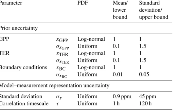
Table 3. Probability density functions (PDFs) for parameter and hyper-parameter scaling factors. Mean and standard deviation in the fourth and fifth columns relate to log-normal PDFs; lower bound and upper bound relate to uniform PDFs.
Parameter PDF Mean/ Standard lower deviation/ bound upper bound Prior uncertainty
GPP xGPP Log-normal 1 1
σxGPP Uniform 0.1 1.5
TER xTER Log-normal 1 1 σxTER Uniform 0.1 1.5
Boundary conditions xBC Log-normal 1 1 σxBC Uniform 0.01 0.05
Model–measurement representation uncertainty
Standard deviation σy Uniform 0.9 ppm 45 ppm
Correlation timescale τ Uniform 1 h 120 h
periods resolved in the inversion, which is important because CO2fluxes vary strongly in time and have high uncertainty
in their temporal variation.
In general, there is no analytical solution to our hierarchi-cal Bayesian equation, so we approximate the posterior so-lution using a reversible jump Metropolis–Hastings MCMC algorithm (Metropolis et al., 1953; Green, 1995; Tarantola, 2005; Lunt et al., 2016). The algorithm explores the possi-ble values for each parameter by making a new proposal for a parameter value at each step of a chain of possible val-ues. Proposals are accepted or rejected based on a compar-ison between the current and proposed state’s fit to the data (likelihood ratio), deviation from the prior PDF (prior ratio) and a term governing the probability of generating the pro-posed state versus the reverse proposal (proposal ratio). More favourable parameter values or model states are always ac-cepted; however, less favourable parameter values or model states can be randomly accepted in order to fully explore the full posterior PDF. The algorithm had a burn-in period of 5 × 10⁴iterations and was then run for an additional 2 × 10⁵ iterations to appropriately explore the posterior distribution. At the end of the algorithm a chain of all accepted param-eter values is stored (if a proposal is rejected the chain will spend longer at the previously accepted value). A histogram of this chain describes a posterior PDF for each parameter so that statistics such as the mean, median and standard devia-tion can be calculated. The trace of each chain was examined qualitatively to ensure that the algorithm had been run for a sufficient number of iterations to converge on a result. 2.4.2 Basis functions
Our domain is split into five spatial regions separating west-central Europe from north-east, south-east, south-west and north-west regions, shown in Fig. S1. Within the west-central Europe area (the hatched region in Fig. S1), a map of the
frac-tion of different plant funcfrac-tional types in each grid cell has been used to further break down the region (Fig. S6). This is the same PFT map used in the JULES biospheric simula-tion (see Sect. 2.3.2). A scaling factor is solved in the inver-sion, scaling GPP and TER within the four outer regions and within maps of five or six PFTs in the subdomain: broadleaf tree; needleleaf tree; C3grasses; C4grasses; shrubland; and,
in the case of TER, bare soil. Therefore there are 19 spatial basis functions in total.
2.4.3 Definition of Jacobian matrix
Footprints from NAME, prior fluxes, boundary conditions and basis functions are all combined into a matrix of partial derivatives, alternatively described as a “Jacobian” or “sensi-tivity” matrix, that describes the change in mole fraction with respect to a change in each of the input parameters. This is the “model” in the inversion set-up, denoted H in the de-scription of the linear forward model (Eq. 7), where ε is the mismatch between modelled observations and what has actu-ally been measured in the atmosphere. H has dimensions m (number of data points) by n (number of parameters).
y = Hx + ε (5)
To create this linear model, we multiplied the footprints by the prior GPP and TER fluxes separately and then multiplied these by the fractional map of basis functions (described in Sect. 2.4.2) and summed over the domain. The boundary con-ditions were broken down by four further basis functions for each edge of the domain as explained in Sect. 2.2.2. The pa-rameters vector, x, consisted of a set of scaling factors that multiplied the fluxes or boundary conditions. Multiplying the sensitivity matrix by the prior estimate of x, a vector of ones, yields the prior modelled mole fraction time series at a site. Therefore, during our inversion, we are updating this vector of ones as a scaling factor, to scale up or down emissions for each PFT and biospheric component to better agree with the data. Whilst in theory we have posterior information about the gross GPP and TER biospheric components separately, we combine this into a net ecosystem exchange (NEE) flux estimate, as we believe this to be more robust (Tolk et al., 2011). Therefore, throughout this paper we discuss posterior NEE estimates; however, the results of the separate sources can be found in the supplement in Figs. S7–S9.
3 Results
We have applied our CO2inversion set-up to UK biospheric
CO2flux estimation using output from two different models
of biospheric flux as a prior constraint in two inversions. We first describe differences between the output from the two prior models and then present the UK flux estimates found with this method, along with the spatial distribution of pos-terior fluxes.
3.1 Differences between DALEC and JULES
The CO2fluxes from DALEC and JULES differ both
tem-porally and spatially. Figure 2a–c shows UK fluxes of GPP, TER and NEE from the two models. Most notable differ-ences are seen in TER where JULES has a large diurnal range, whereas DALEC has a small diurnal range. Averaged to monthly resolution, the fluxes are relatively similar al-though DALEC has a higher TER flux from July to Octo-ber. Diurnal ranges for GPP are more similar in magnitude; however, JULES exhibits a stronger sink in spring with max-imum uptake in June. DALEC has maxmax-imum uptake in July and exhibits a stronger sink in autumn. Combining these two fluxes, we can see that the profile of NEE for both models is quite different. The daily maximum source from JULES remains relatively constant throughout the year, whereas the daily maximum source in DALEC follows a similar seasonal cycle to the daily maximum sink (albeit with a smaller mag-nitude). Monthly net fluxes are similar between both models for much of the year although JULES has stronger uptake between March and June.
In order to understand some of these seasonal differences it is useful to compare the processes taking place in each model. Section 2.3.1 and 2.3.2 provide detailed descriptions of each model and we give an overview of the main differ-ences here. DALEC explicitly simulates the soil and litter stocks, growth and turnover processes. LAI is estimated by DALEC at a weekly time step; DALEC was calibrated us-ing MODIS LAI estimates at the correct time and location of the analysis, explained in Sect. 2.3.1. In the JULES sys-tem, soil and litter carbon stocks are fixed values for each grid cell, calibrated from 1990 to 2000, and a fixed climatology of MODIS LAI and canopy height is used. Therefore, DALEC has interannual variability in LAI and soil carbon stocks and can adjust the parameters to find the most likely estimates in combination with other data, whereas these parameters re-main constant in JULES. This is potentially advantageous for DALEC, although the use of a climatology in JULES means that noise in the MODIS LAI estimates will be aver-aged out. Since LAI and soil and litter carbon stocks are fixed in JULES, variability in TER and GPP fluxes is governed by meteorology – primarily temperature but also significant signals from photosynthetically active radiation and precip-itation via the soil moisture. Meteorology drives the JULES model at a 2-hourly time step as opposed to a weekly time step in DALEC. Therefore, in the 2-hourly DALEC product used here, the diurnal range is not explicitly simulated and is the result of a downscaling process from a weekly res-olution. This downscaling is done based on light and tem-perature curves as explained in Sect. 2.3.1. In DALEC, the autotrophic respiration is parameterised as a fixed fraction of the GPP for a given site but varies between sites, roughly ranging from 0.3 to 0.7. In JULES, the autotrophic respi-ration is the sum of plant maintenance and growth respira-tion terms, which are calculated separately as process-based
functions of the GPP, the maximum rate of carboxylation and leaf nitrogen content (Clark et al., 2011). Typically, the autotrophic respiration in JULES is roughly 0.1–0.25 of the GPP. Therefore, there are some large differences between the model structures and parameterisations, particularly in how the respiration fluxes are simulated. This could be leading to too small a diurnal range in DALEC TER and too large a diurnal range in JULES TER.
Figures 3 and 4 show spatial maps of GPP, TER and NEE from both models averaged over winter (December, Jan-uary, February) and summer (June, July, August) months. The pattern of TER is similar for both models; however, JULES always has a stronger source over Northern Ireland and DALEC has a stronger source in east England. In winter there are only small spatial variations in DALEC GPP fluxes, whereas JULES has its largest uptake in south-west England and Wales. In summer, the models are roughly in agreement in the size of the sink in Wales and the majority of England; however, JULES has a stronger sink in Scotland and North-ern Ireland and DALEC has a stronger sink in central and south-east England. The differences between the models in GPP and TER lead to fairly different winter NEE flux maps. DALEC is a net source everywhere in winter, with areas of strongest net source in southern Scotland as well as east and central England. JULES is a small net winter sink in North-ern Ireland, Wales, and south and central England. Summer NEE fluxes are similar between the models, although JULES has a stronger net sink in Scotland and Northern Ireland. 3.2 Posterior net UK biospheric CO2flux 2013–2014
We have derived estimates for annual NEE from the UK using CO2 flux output from the two different
mod-els of biospheric flux as prior information (Fig. 5 – or-ange and blue bars for DALEC and JULES respectively): 13±9087Tg CO2yr−1(DALEC prior) and 76±9190Tg CO2yr−1
(JULES prior) in 2013 and 2±7068Tg CO2yr−1 (DALEC
prior) and 51±8078Tg CO2yr−1(JULES prior) in 2014. These
annual net flux estimates from both models agree within the estimated uncertainties, and mean values are higher than their respective priors in both cases. The uncertain-ties straddle the zero net flux line, implying that the UK is roughly in balance between sources and sinks of bio-spheric CO2. However, according to the inversion using
JULES, a net biospheric source is less likely than in the inversion using DALEC. When added to the anthropogenic and ocean fluxes that remained fixed during the inversion, we produce the following estimates for annual total net CO2 release from the UK (Fig. 5 – yellow and green bars
for DALEC and JULES respectively): 448±9087Tg CO2yr−1
(DALEC prior) and 386±9190Tg CO2yr−1 (JULES prior)
in 2013 and 418±7068Tg CO2yr−1 (DALEC prior) and
369±8078Tg CO2yr−1 (JULES prior) in 2014. While we are
assuming that anthropogenic and ocean fluxes are perfectly known, the uncertainties on these fluxes are comparatively
Figure 3. Average prior flux maps for winter 2013 (December 2013, January–February 2014). (a) TER from DALEC; (b) TER from JULES; (c) the difference between DALEC and JULES TER; (d) GPP from DALEC; (e) GPP from JULES; (f) the difference between DALEC and JULES GPP; (g) NEE from DALEC; (h) NEE from JULES; (i) the difference between DALEC and JULES NEE.
small (Peylin et al., 2011). When the anthropogenic source was varied by ±10 %, a conservatively large estimate of these uncertainties, we found posterior biospheric flux estimates using the DALEC prior that still suggest a balanced bio-sphere and posterior flux estimates using the JULES prior that suggest a small net sink at the lowest end of the possibil-ities explored here (see Fig. S10). All mean annual posterior estimates, regardless of the anthropogenic source used, sug-gest the prior net biospheric flux is underestimated; i.e. pos-terior biospheric uptake of CO2is smaller than predicted by
the models. However, this is less statistically significant with the 2013 inversion using the DALEC prior.
The monthly posterior UK estimates using both models (Fig. 5) mostly agree well with each other within the un-certainties; however, they are both notably different from the prior estimates, especially in 2014. The posterior total UK flux estimate, achieved by adding the posterior NEE fluxes to anthropogenic and coastal ocean fluxes, shows that, according to the DALEC inversion, the UK may not be a net sink of CO2at any time of year in 2013 and 2014. However,
the JULES inversion suggests the UK is a net sink of CO2in
June of both years.
Posterior seasonal cycle amplitudes are generally smaller than the prior amplitudes, except in the DALEC inversion in 2014. Table 4 gives the posterior maximum and min-imum values of NEE, leading to seasonal cycle ampli-tudes of 469 and 578 Tg CO2yr−1 for 2013 and 633 and
737 Tg CO2yr−1for 2014, for the DALEC and JULES
in-versions respectively. These values are 90 % and 76 % of the prior amplitudes in 2013 and 123 % and 85 % of the prior amplitudes in 2014.
The largest differences between the prior and posterior are seen in spring and summer for both models. Posterior UK NEE estimates from the DALEC inversion are in agree-ment with the prior for 11 months: during the first half of 2013, in the majority of winter months (December, Jan-uary, February) and in June 2014. When the DALEC in-version posterior UK NEE estimates are not in agreement with the prior, they are usually larger, with a maximum dif-ference in 2013 of 235±9291Tg CO2yr−1 in August and a
maximum difference in 2014 of 551±8084Tg CO2yr−1in July,
although in spring (March, April, May) 2014 they tend to be smaller than the prior, with a maximum difference of −194±6460Tg CO2yr−1in April. Posterior UK NEE from the
Figure 4. Prior average flux maps for summer 2014 (June–August 2014). (a) TER from DALEC; (b) TER from JULES; (c) the difference between DALEC and JULES TER; (d) GPP from DALEC; (e) GPP from JULES; (f) the difference between DALEC and JULES GPP; (g) NEE from DALEC; (h) NEE from JULES; (i) the difference between DALEC and JULES NEE.
Table 4. Posterior UK estimates for the maximum net biospheric source and sink (values also shown in Fig. 5). The month in brackets indicates the month in which the maximum source or sink occurred.
Year Maximum sink (Tg CO2yr−1) Maximum source (Tg CO2yr−1)
DALEC 2013 −298±140136(June) 171±9476(January) 2014 −360±8788(June) 273±6563(November) JULES 2013 −456±9091(June) 122±8378(December)
2014 −542±97100(June) 195±6570(October)
the 2-year period, the majority of which is between Novem-ber and February. Otherwise, the posterior estimate from the JULES inversion is larger than the prior, with a maximum difference in 2013 of 318±7071Tg CO2yr−1 in April and a
maximum difference in 2014 of 407±7672Tg CO2yr−1in July.
Looking at the spring and summer differences more closely, we find that the JULES model has a systemat-ically lower net spring flux than the posterior, and the DALEC model is either in agreement with or higher than the posterior estimate of the net spring flux. Generally, the models underestimate the net summer flux compared to the posterior flux (to the greatest extent in 2014), al-though the summer estimate from the JULES inversion
in 2013 is not statistically different from the prior. The average spring difference between the posterior and the prior for the DALEC inversion is −2±8988Tg CO2yr−1
in 2013 and −133±6763Tg CO2yr−1 in 2014, whereas for
the JULES inversion it is 219 ± 87 Tg CO2yr−1 in 2013
and 164±6765Tg CO2yr−1in 2014. The average summer
dif-ference for the DALEC inversion is 135±111108Tg CO2yr−1
in 2013 and 263±8283TgCO2yr−1 in 2014, whereas for the
JULES inversion it is 94±104107Tg CO2yr−1in 2013 and 312±
85 Tg CO2yr−1in 2014. The prior sink in June as estimated
by the JULES model is nearly twice that of DALEC and pos-terior estimates tend to agree with the DALEC prior in this month.
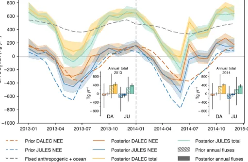
Figure 5. Posterior monthly net UK CO2 flux (positive is emission to atmosphere). Orange and blue monthly fluxes are posterior net
biospheric (NEE) fluxes for DALEC and JULES respectively. Prior biosphere fluxes from DALEC and JULES are shown in dashed orange and blue lines respectively. The fixed anthropogenic and ocean fluxes are denoted by the dark grey dashed line. Yellow and green monthly fluxes are the sum of the posterior NEE fluxes and the fixed anthropogenic and ocean fluxes. Shading represents 5th–95th percentile. The bar charts represent annual net UK CO2flux for 2013 (left) and 2014 (right). Hashed bars denote prior annual fluxes; solid bars denote posterior
annual fluxes. The bar colours correspond to the line colours: left-hand bars for each model are NEE fluxes; right-hand bars for each model are total fluxes (NEE + fixed sources). Uncertainty bars represent 5th–95th percentile. DA – DALEC. JU – JULES.
Figure S9c shows the daily minimum and maximum in the posterior net biospheric estimates for 2014. It is worth bear-ing in mind at this point that while the temporal resolution of the inversion is flexible, it can go down to a minimum reso-lution of 1 day (as explained in Sect. 2.4.1). Therefore, the diurnal profile of TER and GPP for each model is imposed; however, it can be scaled up or down from day to day. Fig-ure S11 shows that the inversion typically scaled the fluxes within 4 or 5 temporal regions per month, although for some parameters in some months scaling factors were found up to roughly a daily resolution. For both inversions, the posterior NEE flux shown in Fig. S9c has a similar profile. Compared to Fig. 2c the inversion tends to a seasonal cycle in daily max-imum uptake that resembles that of the JULES model prior, with a turning point in maximum uptake occurring abruptly between June and July, a steep gradient in spring and a shal-low gradient in autumn. On the other hand, the seasonal cy-cle in daily maximum source resembles that of the DALEC model prior, which has a stronger seasonal variation com-pared to that of the JULES model prior, albeit with a larger amplitude. This would suggest that the underestimation in net spring flux seen in the JULES prior is generally due to the model underestimating the spring source rather than over-estimating the spring sink. It also suggests that the overesti-mation in net summer flux in the DALEC prior is possibly a combination of the model overestimating the summer sink and underestimating the summer source. The overestimation
in the net summer flux in JULES is more likely to be due to an underestimation of the summer source. However, as di-urnal fluxes vary on a scale nearly an order of magnitude larger than that of the monthly fluxes, it is clear that any rel-atively small changes in the maximum source or sink will have a relatively large effect on the daily net flux. Therefore, the monthly net flux is the more robust result here and we are not able to confidently draw conclusions from the sub-monthly results.
3.3 Posterior spatial distribution of biospheric fluxes Figure 6 shows mean posterior net biospheric fluxes (NEE) for winter 2013 and summer 2014 from both the DALEC and JULES inversions. In winter 2013, posterior NEE fluxes from the DALEC inversion are fairly heterogeneous and are largest over south-west Scotland and east and central Eng-land. This posterior spatial distribution is roughly similar to the prior. From the inversion using JULES prior fluxes, the posterior net biospheric flux is much smoother than it is for the inversion using DALEC. It is largest in north-west Eng-land and almost zero in east EngEng-land. The whole of south and central England, Wales, and Northern Ireland have increased posterior winter fluxes compared to the prior, turning these areas from a net sink in the prior to a net source in the poste-rior.
Figure 6. Posterior net biospheric (NEE) flux maps averaged over winter 2013 (December 2013, January–February 2014) and summer 2014 (June–August 2014). (a) Winter NEE flux from DALEC inversion. (b) Winter NEE flux from JULES inversion. (c) Difference between winter NEE flux from DALEC (DA) and JULES (JU) inversions. (d) Summer NEE flux from DALEC inversion. (e) Summer NEE flux from JULES inversion. (f) Difference between summer NEE flux from DALEC (DA) and JULES (JU) inversions.
In summer 2014, NEE fluxes from the two inversions dis-play many similarities, with areas of net source in east, cen-tral (extending further south in the JULES inversion), and north-west England and areas of net sink elsewhere. How-ever, the net sink in the JULES inversion is larger than the DALEC inversion in Scotland, south Wales, Northern Ire-land and south-west EngIre-land. This differs from the prior flux maps, which have only very small areas of small net uptake in central England in DALEC and in east England in JULES. Both the DALEC and JULES posterior fluxes generally dis-play reduced uptake compared to the prior, except in north Wales.
3.4 Model–data comparison
Agreement between the data and the posterior simulated mole fractions at the measurement sites used to constrain the inversion is greatly improved compared to prior simulated mole fractions, with R2 values increasing by a minimum of 0.24 and up to 0.5 (to give values ranging between 0.53 and 0.71) and root mean square error (RMSE) decreasing by at least 1.35 ppm and up to 2.6 ppm (to give values ranging between 1.26 and 2.71 ppm). Table 5 shows all statistics for the prior and posterior mole fractions compared to the obser-vations of atmospheric CO2concentrations. Overall, the fits
are relatively similar between the DALEC and JULES in-versions, implying that the two inversions perform similarly well by these metrics. In terms of R2, the best fit to the data is observed at Heathfield in the DALEC inversion and
An-gus in the JULES inversion. In terms of RMSE, the best fit to the data is observed at Angus in the DALEC inversion and Mace Head in the JULES inversion. The smallest posterior mean bias is observed at Angus in the DALEC inversion and Ridge Hill in the JULES inversion. Therefore, there are some small spatial differences in how well each of the inversions is able to fit the data but no clear indication of which areas of posterior flux might be subject to the largest improvement in either inversion. Figures S12 and S13 show the residual mole fractions in 2014 and indicate that residuals are some-what larger during the summer than the winter.
To test our posterior results against data that have not been included in the inversion, the posterior fluxes have been used to simulate mole fractions at Weybourne Atmospheric Ob-servatory (see Fig. 1 for location in relation to the other sites and Table 1 for site information). The statistics of fit to the data are given in italics in Table 5 and show an improve-ment in R2of 0.18 with the DALEC inversion and 0.13 with the JULES inversion, an improvement in RMSE of 1.09 ppm with the DALEC inversion and 0.75 ppm with the JULES in-version, and an improvement in the mean bias of 0.64 ppm in the DALEC inversion and 0.56 in the JULES inversion. These results show that the a posteriori fluxes improve the fit to the data at a measurement station not included in the inversion. The results are very similar between the two inver-sions at this site but suggest that the DALEC inversion may perform slightly better, at least in this region of the UK. Fig-ure S14 shows the residual mole fractions at Weybourne for each of the inversions carried out in this work.
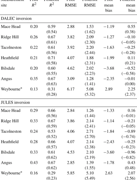
Table 5. Prior and posterior fit to data statistics for the inversion period 2013–2014. R2and RMSE are calculated monthly and averaged over this period. Values in brackets are the posterior fit statistics for the corresponding net flux inversions.∗Weybourne data (from February to December 2013) were used for validation of the results only and were not included in the inversions.
Measurement Prior Posterior Prior Posterior Prior Posterior site R2 R2 RMSE RMSE mean mean bias bias DALEC inversion Mace Head 0.20 0.59 2.88 1.53 −1.19 0.55 (0.54) (1.62) (0.38) Ridge Hill 0.26 0.67 3.82 2.09 −1.27 −0.10 (0.61) (2.30) (−0.05) Tacolneston 0.22 0.61 3.92 2.20 −1.63 −0.25 (0.56) (2.44) (−0.28) Heathfield 0.21 0.71 4.07 1.88 −1.99 0.11 (0.58) (2.31) (0.21) Bilsdale 0.20 0.60 4.62 2.02 −3.68 −0.52 (0.55) (2.23) (−0.58) Angus 0.35 0.67 3.09 1.28 −2.35 −0.01 (0.63) (1.41) (0.00) Weybourne∗ 0.13 0.31 6.17 5.08 2.89 2.25 (0.28) (5.32) (2.37) JULES inversion Mace Head 0.29 0.66 2.84 1.26 −1.33 0.16 (0.56) (1.44) (−0.01) Ridge Hill 0.33 0.67 3.86 2.14 −1.14 −0.21 (0.59) (2.41) (−0.05) Tacolneston 0.24 0.53 4.06 2.71 −1.84 −0.89 (0.52) (2.70) (−0.74) Heathfield 0.28 0.66 4.07 2.14 −2.43 −0.25 (0.57) (2.38) (−0.23) Bilsdale 0.33 0.61 4.53 2.10 −3.60 −0.96 (0.62) (2.19) (−0.82) Angus 0.43 0.67 2.85 1.39 −1.78 0.43 (0.62) (1.55) (0.48) Weybourne∗ 0.16 0.29 5.85 5.10 2.63 2.07 (0.23) (5.49) (2.56) 4 Discussion 4.1 Inversion performance
Solving for both TER and GPP separately allows the JULES prior and DALEC prior inversions to converge to a similar posterior solution. Using two very different prior NEE flux estimates, we produce two similar posterior NEE flux esti-mates that have a similar seasonal amplitude and agree on the majority of monthly and all annual fluxes within the es-timated uncertainties. This indicates that our posterior esti-mates are driven by the data rather than determined by the prior. However, when we carry out the same inversion but scale NEE (Fig. S15) we find the two posterior flux estimates do not converge on a common result. The posterior seasonal cycles remain relatively unchanged compared to the prior and
annual net biospheric flux estimates tend to be similar to, or larger than, the prior. These annual net biospheric flux es-timates are therefore 3–39 times smaller than the inversion that separates GPP and TER, meaning the posterior estimates from the two types of inversions do not overlap, even within estimated uncertainties. Evaluating the statistics of how well the NEE inversions fit the data (Table 5), we find they do not perform as well as the separate GPP and TER inversion, both at the sites included in the inversion and at the validation site, WAO. However, this is to be expected to some degree, because separating the two sources gives the inversion more degrees of freedom to fit the data.
As recommended by Tolk et al. (2011), we are only hoping to achieve an improved estimate for the net fluxes here rather than the gross GPP and TER fluxes themselves. The posterior gross fluxes are included in the supplement (Figs. S7–S9),
but due to the correlation between the spatial and temporal distribution of GPP and TER they have not been presented in the main text. This can be seen in summer and winter flux maps (Figs. S7 and S8) and in the posterior annual flux esti-mates in Fig. S9d, in particular where JULES TER and GPP show similarly large differences from the prior. This could also be a result of the imposed diurnal cycle, as it would ap-pear the posterior TER flux in the JULES inversion is tend-ing to a higher daily minimum, matchtend-ing that of the DALEC prior, and may ultimately be trying to move towards a smaller diurnal variation in TER. However, because the whole diur-nal cycle must be scaled, the daily maximum TER must also increase and may mean the GPP must increase, causing in-creased uptake, to compensate for the inin-creased source from TER. Allowing flexibility on sub-daily timescales may lead to similar estimates of GPP and TER between the two inver-sions with different priors. However, questions remain over whether there is enough temporal information for this to be the case.
The fact that common monthly and annual posterior net biospheric flux estimates are reached when the prior bio-spheric fluxes are spatially and temporally different would suggest that the choice of prior is not necessarily a major factor in guiding the inversion result for our network, when GPP and TER are scaled separately. In this respect, it is also particularly encouraging that the seasonal cycles in the pos-terior diurnal range are similar for both inversions (Fig. S9c). 4.2 Differences between prior and posterior
NEE estimates
The posterior seasonal cycle in both inversions differs signifi-cantly from the prior. This implies that the biospheric models used to obtain prior GPP and TER fluxes are either over- or underestimating the strength of some processes, or they are omitting some processes altogether. The largest differences between the posterior solution and the prior model output are seen in spring and summer. In Sect. 3.2 we have shown that spring differences arise from an overestimation of the net spring uptake of CO2in the JULES model and an
under-estimation of the net spring uptake in the DALEC model in 2014. However, in summer (particularly in 2014), the pos-terior net UK fluxes are higher than both priors in July and August.
One process that occurs during the months July and Au-gust is crop harvest. Harvest is not directly resolved in either of the models of the biosphere used in this work, thereby providing a possible explanation for the differences between the posterior and prior in these months. Harvest typically occurs between July and September and arable agricultural land covered 26 % of the UK in 2013 and 2014 (DEFRA, 2014, 2015), so there is potential for unaccounted activity in this area to cause large changes to net CO2 fluxes. The
areas of net source in summer (shown in Fig. 6) do also coincide with areas of large-scale agriculture (e.g. east and
central England). Crop harvest potentially changes the bio-sphere in the following ways: firstly, crops mature en masse, leading to an abrupt loss of productivity. Secondly, during harvest there is an abrupt removal of biomass and input of harvest residues on the field. This increases litter input that is readily available for decomposition, increasing heterotrophic respiration. Thirdly, when the field is ploughed the soil is disturbed, which can increase heterotrophic respiration. Fi-nally, when the crop is no longer covering the soil surface this layer can become drier and the energy balance is al-tered. In Smallman et al. (2014), the reduction in atmospheric CO2 concentration due to crop uptake is reported for 2006
to 2008 and an abrupt increase in atmospheric CO2can be
seen between June (peak source) and August, where CO2
uptake from crops is halted as a result of harvest. Harvest may explain the abrupt shift from net sink to net zero or net source observed between July and August in DALEC in 2013 and June and July in both models in 2014. The earlier time in 2014 does coincide with a year of early harvest (DEFRA, 2015) although this may well be fortuitous. Later in the sum-mer, there may be some plant regrowth in ploughed fields leading to increased GPP. This would be consistent with the shallower gradient observed in net biospheric fluxes between September and October 2013 in the DALEC posterior esti-mate, between August and September 2014 in the JULES posterior estimate, and the decrease in net flux observed be-tween July and September 2014 in the DALEC posterior es-timate.
If agricultural activity is the source of the July, August and September difference between prior and posterior UK NEE estimates, then it could amount to emissions of 4 %–10 % of currently reported annual anthropogenic emissions in 2013 and 17 %–19 % in 2014. However, other explanations for this difference could be large uncertainties in the seasonal disag-gregation of anthropogenic fluxes, uncertainties in the trans-port model, or a combination of over- and underestimation of other biospheric processes.
4.3 Implications for UK CO2emissions estimates
The results of UK biospheric CO2 fluxes using our set-up
suggest the UK biosphere is roughly in balance, whereas prior estimates from models of the biosphere estimate a net sink. Even when we assume an uncertainty on our anthro-pogenic fluxes of 10 % (a conservative estimate), inversions using both models still give mean posterior estimates that are larger than their respective priors (see Fig. S10). Therefore, when using models of the biosphere to contribute to inven-tory estimates of CO2 emissions, care must be taken to
at-tribute sufficient uncertainties to model estimates, otherwise the amount of CO2taken up by the biosphere on an annual
basis may be overestimated. Methods such as the one de-scribed in this paper could provide an important constraint on the UK’s biospheric CO2 fluxes as carbon sequestration