Magnetopause mapping to the ionosphere for northward IMF

HAL Id: hal-00318426

https://hal.archives-ouvertes.fr/hal-00318426

Submitted on 2 Jan 2008

HAL is a multi-disciplinary open access

archive for the deposit and dissemination of

sci-entific research documents, whether they are

pub-lished or not. The documents may come from

teaching and research institutions in France or

abroad, or from public or private research centers.

L’archive ouverte pluridisciplinaire HAL, est

destinée au dépôt et à la diffusion de documents

scientifiques de niveau recherche, publiés ou non,

émanant des établissements d’enseignement et de

recherche français ou étrangers, des laboratoires

publics ou privés.

IMF

I. I. Alexeev, E. S. Belenkaya, S. Yu. Bobrovnikov, V. V. Kalegaev, J. A.

Cumnock, L. G. Blomberg

To cite this version:

I. I. Alexeev, E. S. Belenkaya, S. Yu. Bobrovnikov, V. V. Kalegaev, J. A. Cumnock, et al..

Magne-topause mapping to the ionosphere for northward IMF. Annales Geophysicae, European Geosciences

Union, 2008, 25 (12), pp.2615-2625. �hal-00318426�

www.ann-geophys.net/25/2615/2007/ © European Geosciences Union 2007

Annales

Geophysicae

Magnetopause mapping to the ionosphere for northward IMF

1_{Skobeltsyn Institute of Nuclear Physics, Moscow State University, Moscow, Russia}

2_{Space and Plasma Physics, School of Electrical Engineering, Royal Institute of Technology, Stockholm, Sweden} 3_{Center for Space Sciences, University of Texas at Dallas, Richardson, TX, USA}

Received: 2 March 2007 – Revised: 6 September 2007 – Accepted: 30 October 2007 – Published: 2 January 2008

Abstract. We study the topological structure of the magneto-sphere for northward IMF. Using a magnetospheric magnetic field model we study the high-latitude response to prolonged periods of northward IMF. For forced solar wind conditions we investigate the location of the polar cap region, the polar cap potential drop, and the field-aligned acceleration poten-tials, depending on the solar wind pressure and IMF By and Bxchanges. The open field line bundles, which connect the Earth’s polar ionosphere with interplanetary space, are calcu-lated. The locations of the magnetospheric plasma domains relative to the polar ionosphere are studied. The specific fea-tures of the open field line regions arising when IMF is north-ward are demonstrated. The coefficients of attenuation of the solar wind magnetic and electric fields which penetrate into the magnetosphere are determined.

Keywords. Magnetospheric physics (Auroral phenomena, Magnetospheric configuration and dynamics, Solar wind-magnetosphere interactions)

1 Introduction

The polar cap can, as a first approximation, be considered a region void of precipitating particles inside the auroral oval. However, during northward interplanetary magnetic field (IMF), several different types of high-latitude emis-sions have been observed (Kullen et al., 2002), including transpolar aurora (TPA). The TPAs cross the noon-midnight meridian only when By changes sign, resulting in a large Bz/|By|ratio. The theta aurorae form in the Northern Hemi-sphere, from an expanded dawnside (duskside) emission re-gion when Bychanges from negative to positive (positive to negative) (Cumnock et al., 1997, and references therein).

Correspondence to: I. I. Alexeev

(iialexeev@mail.ru)

It is clear that energetic (up to several keV) particle precip-itation is the cause of these emissions, although the source of them remains unknown. The precipitating particles may be accelerated by a magnetic field-aligned potential drop (Lyons 1980; Carlson and Cowley 2005), or may be a consequence of pitch-angle scattering of the magnetospheric plasma sheet particle populations due to stretched tail-like field lines at the current sheet. The visible and UV emissions can be driven by one or both mechanisms. Either way, the energy source of the auroral particle fluxes is the solar wind flow past the magne-tosphere. The magnetospheric field line geometry is highly complex in the northward IMF case, as pointed out, for ex-ample, by Cowley (1973), Alexeev and Belenkaya (1983) (see also Siscoe et al., 2001), and Belenkaya (1998a, b).

Frank et al. (1982, 1986) proposed that theta aurora is lo-cated on closed field lines and is connected with the plasma sheet boundary layer or the distant plasma sheet. On the basis of particle flux data, Peterson and Shelley (1984) also sup-ported the closed field lines idea. Reiff and Burch (1985) explained the high-latitude aurora under northward IMF, as-suming open magnetic flux across the tail lobes.

Reconnection inside the magnetosphere for northward IMF was first described by Alexeev and Belenkaya (1983) and later called by Siscoe (1988) “the current penetration model”. The reconnection x-line for northward IMF trans-forms into two magnetic field neutral points where 3-D re-connection occurs near the cusps (Alexeev and Belenkaya, 1983).

The portion of the IMF that penetrates into the magneto-sphere is only a small part of the average magnetospheric magnetic field. However, this small field strongly controls the outer magnetosphere structure. For Bz<0, the recon-nection region is located in the equatorial part of the day-side magnetopause, and in the magnetotail, while for Bz>0, two reconnection sites are located in the cusp regions (see, for example, Alexeev and Belenkaya, 1985). The conse-quences of the transformation from southward to northward

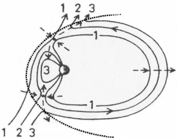
Fig. 1. We have followed Dungey’s (1963) ideas which were later described by Cowley (1983), who represented the sequential merg-ing in the Northern and Southern Hemisphere for the cases of IMF

Bx<0. We have drawn on Fig. 1e from Cowley (1983) a dotted

curve which indicates the magnetopause. Lobe reconnection first occurs in the Northern Hemisphere, forming an open field line that drapes over the dayside and one that connects to the Southern Hemi-sphere. Later, the overdraped field line merges with one of the pre-viously opened field lines in the Southern Hemisphere, forming a closed dayside field line and a completely detached IMF field line (see also Belenkaya, 1998a, b).

IMF cases are not limited to moving the reconnection site from the equatorial dayside magnetopause to the cusp region. The overall topology of the IMF and magnetospheric field reconnection is different for northward and southward IMF directions (Alexeev, 1986; Belenkaya, 1998a, b).

The theme of this paper is internal reconnection for north-ward IMF. Our analysis is based on a long history of model-ing of magnetospheric mergmodel-ing configurations, for example, see reviews by Siscoe (1988) and Crooker (1990). In this paper we refer to one of the simplest models classified by Siscoe (1988) as a current penetration model (Alexeev and Belenkaya, 1983) (see also Crooker, 1990, 1992; Crooker et al., 1998). In addition to superposing a dipole field and a uniform field (IMF) (Dungey, 1963; Cowley, 1973; Stern, 1973) this model associates the merging process with a mag-netospheric boundary current through which the interplane-tary magnetic field penetrates the magnetosphere. For north-ward IMF, at some point in the cusp region inside the mag-netosphere, the penetrated IMF and the magnetospheric field cancel each other. At the neutral point of the magnetic field three-dimensional reconnection occurs. A short description of this model is given in the next section.

We follow the line of Dungey (1963) and Cowley (1983). In our approach, similar to the northward IMF reconnection scenario shown in Fig. 1 from Cowley (1983), two neutral points exist near the northern and southern cusps. The open

field lines appear at one neutral point, as a result of recon-nection of the IMF lines penetrated into the magnetosphere and closed field lines. Later, the open field lines of both po-lar caps reconnect, forming closed and IMF field lines. The reconnection for different IMF orientations is considered by us in detail in a set of papers for the Terrestrial, Jovian and Kronian magnetospheres (e.g. Alexeev and Belenkaya, 1985, 1989; Belenkaya, 1993, 1998a, b, 2004; Belenkaya et al., 2006; Belenkaya et al., 2006a, b).

Figure 1 presents Cowley’s (1983) representation of se-quential merging in the Northern and Southern Hemispheres (see Fig. 1e in Cowley, 1983). Lobe reconnection first occurs in the Northern Hemisphere, forming an open field line that drapes over the dayside and one that connects to the Southern Hemisphere. Later, the overdraped field line merges with one of the previously opened field lines in the Southern Hemi-sphere, forming a closed dayside field line and a completely detached field line. Similar sequential merging can also oc-cur in the case of open field lines in the tail, though this is not illustrated in the Fig. 1.

We assume that, with the exception of a relatively small diffusion region near the neutral point, the magnetic field lines could be considered as equipotential. In the diffu-sion region, a field-aligned potential drop appears. Here we concentrate on quantitative calculations of the magnetic and electric fields near the high-latitude reconnection site for northward IMF. Based on the dynamic magnetospheric model, quantitatively taking into account the IMF penetra-tion into the magnetosphere, we will map the solar wind elec-tric potential along the magnetic field lines to ionospheric al-titudes.

2 Model description

The current penetration model of the IMF and magneto-spheric magnetic field merging was proposed by Alexeev and Belenkaya (1983) and was later developed by Crooker et al. (1990) (see also Siscoe, 1988). As a consequence of the high (but not infinite) solar wind plasma conductivity, σ , the normal component of the magnetopause magnetic field is nonzero, and proportional to R−m1/4(Alexeev, 1986). The magnetic Reynolds number, Rm=µ0σ VR1, is determined by

the magnetopause subsolar distance, R1, by the solar wind

velocity V , and by the effective conductivity σ of the solar wind plasma. The solution inside the magnetosphere, found by Alexeev (1986), is a spatially uniform magnetic field pen-etrated into the magnetosphere, given by Bn∼Rm−1/4.

Dorelli et al. (2004) also demonstrated that the annihila-tion rate scales, for instance, like R−m1/4 for magnetic re-connection at the terrestrial subsolar magnetopause. Using global MHD simulations, Dorelli et al. (2004) supported the Alexeev (1986) result (Bn∼Rm−1/4), which was obtained analytically, both for a simpler kinetic approach and for the parabolic magnetopause shape. Dorelli et al. (2004)

+ =

Fig. 2. Plasma flow lines and magnetic field lines in the y=0 plane. The x-axis is the Earth-Sun line, the z-axis is parallel to the IMF vector upstream of the bow shock. This coordinate system can be obtained from the solar-magnetospheric coordinates by a rotation around the x-axis. In solar-magnetospheric coordinates, the IMF vector is {Bx, By, Bz}. In IMF-magnetospheric coordinates the

IMF vector is {Bx, 0, Bt}, where Bt= q

By2+Bz2.

demonstrated that if the plasma resistivity is spatially uni-form, magnetic reconnection occurs in the thin current sheet at a rate which is consistent with that predicted by the ana-lytical, incompressible flow solutions (though there are small corrections in simulations due to the plasma compressibil-ity).

Let us demonstrate the IMF draping of the solar wind flow past the magnetosphere for high conductivity of the solar wind plasma. In Fig. 2 (from Alexeev and Kalegaev, 1995) a cross section of the magnetosphere parallel to the IMF (the IMF vector lies in the XZ plane of Fig. 2) is shown. As the magnetospheric magnetic field is precluded from penetrat-ing outside by the magnetopause currents, the magnetic field lines in the magnetosheath do not depend on the mutual ori-entation of the IMF and geomagnetic dipole. Outside the magnetopause, the draping magnetic field (BIMF) can be

cal-culated as a sum of two terms: magnetic field penetrated into the magnetosphere, b, and the part of IMF which is screened by the currents at the magnetopause current layer, Bscr:

BIMF=b + Bscr. (1)

Both parts of the IMF (b and Bscr) have been obtained by

Alexeev et al. (1998). Inside the magnetosphere the solution of the IMF penetration problem is a uniform magnetic field:

b = k||B0||+k⊥B0⊥, (2)

where B0||and B0⊥are the IMF components tangential and

normal to the undisturbed solar wind velocity, V , and k||and k⊥are the screening coefficients for the corresponding IMF components

(k⊥=0.9χ1/2Rm−1/4, and k||=2χ (π Rm)−1/2, respectively). These coefficients depend on the magnetic Reynolds number

Rm, and on the parameter χ =ρ2/ρ1, which determines the

plasma compression at the bow shock (Alexeev et al., 2003); here ρ1is the solar wind plasma density, and ρ2is the

magne-tosheath plasma density downstream of the bow shock. The

= κ

κ

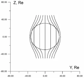
Fig. 3. A projection of the IMF lines on the plane x = R1/2 (where

the paraboloid focus is located) is shown. We see the draping of the magnetic field lines. As a result, the IMF penetrated into the magnetosphere, b=κBB, is only a small part of the IMF upstream

of the bow shock. The factor κBis about 0.1 (Alexeev, 1986), and

it describes the weakening of the IMF inside the magnetosphere.

IMF distortions in the plane perpendicular to the Sun-Earth line are shown in Fig. 3. In this figure the projections of the magnetic field lines on the YZ plane are drawn. We see that as a result of these distortions, only a small part of the elec-tric field potential drop at the magnetospheric diameter can be applied to the polar cap. The effective cross-sectional area of the magnetosphere perpendicular to the Sun-Earth line is smaller than the transverse dimension of the geometric mag-netosphere by a factor κB, equal to the ratio of the penetrated portion of the IMF to the upstream solar wind magnetic field,

κB=k⊥, is the dimensionless factor which describes a de-pression of the interplanetary magnetic field (Bzand By com-ponents), penetrating the magnetosphere (see Eq. 2). The weakening of the solar wind velocity in the boundary layer inside the magnetosphere, near the magnetopause, gives an additional decrease of the penetrated solar wind electric field in κvtimes. This leads to a field-aligned potential drop in the boundary layer region.

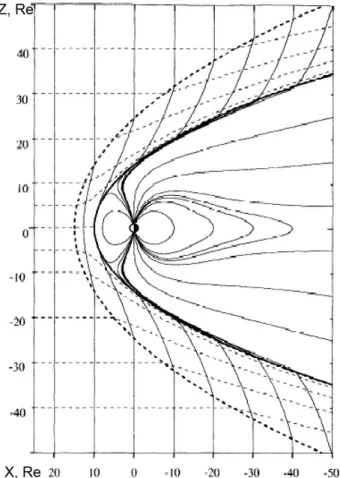
The total picture of the IMF penetrating into the magne-tosphere for southward IMF is shown in Fig. 4 from Alex-eev et al. (1998). The magnetosphere – solar wind inter-action is strongly controlled by the IMF direction, and it is significantly different for northward and southward IMF. However, the disturbances of the IMF and plasma flow in the magnetosheath are similar for both IMF directions in the zero approximation. The undisturbed solar wind region is shown upstream of the bow shock (left side of Fig. 4). Here

Fig. 4. The interplanetary and magnetospheric magnetic field lines in the noon-midnight plane are shown (thin solid curves), as well as the magnetopause (thick solid curve). Upstream of the bow shock and in the magnetosheath we also see the streamlines of the solar wind flowing past the magnetosphere (thin dashed curves).

the velocity and magnetic field are uniform. After the bow shock crossing, the IMF draping by the bow shock and mag-netopause currents is seen. Inside the magnetosphere, we see the shielded field of the internal sources summed with the penetrated IMF b.

In the paraboloid model we represent the magnetopause as a paraboloid of revolution, which is axially symmetric rela-tive to the Sun – Earth line. We will calculate the field lines which cross both the magnetopause and the ionosphere (the open field lines). These field lines can cover only a part of the polar cap; the other part of the black area inside the au-roral oval can be crossed by closed field lines (connecting in both hemispheres) which extend into the distant tail.

The model used here is based on the results of Alex-eev and Belenkaya (1983), AlexAlex-eev (1986), and Belenkaya (1998a, b). For northward IMF, detached IMF lines exist in-side the magnetosphere; they intersect the magnetopause cur-rent sheet two times and do not reach the Earth’s surface (see Fig. 2 in Blomberg et al., 2005). Correspondingly, between the magnetopause current sheet and the open field line bundle

connected with the Earth a bundle of interplanetary magnetic field lines penetrated into the magnetosphere appears. As we speculate here, this is one of the main differences between the southward and northward IMF cases. The reason for this effect is the following: For a closed magnetosphere (when IMF is equal to zero), two neutral points lie on the magne-topause (cusps). For northward IMF, these magnetic nulls cannot stay at the magnetopause. Inside the magnetopause, near the northern cusp, a magnetic field with a north-south component directed to the Earth exists. When the penetrated IMF bz=κBBz>0 is added to the magnetospheric field the northern null moves inside the magnetopause. The coeffi-cient of IMF penetration into the magnetosphere is κB∼0.1 (Alexeev, 1986). Due to a partial IMF penetration inside the magnetosphere, magnetic field neutral points should be shifted inside the magnetosphere to satisfy a condition B=0. Here we take into account the screening effects of the solar wind plasma. Near the magnetic field nulls can be essential in penetrated into the magnetosphere or trapped near cusp plasma. If we study the plasma term by test particle analysis we can show that ion currents only increase northward if bz. Contrary to the northward IMF case, for southward IMF, at the equatorial magnetopause the magnetic field vectors at the magnetosheath and magnetospheric sides of the mag-netopause have opposite directions and a neutral line (con-nected noon and midnight reconnection sites) is placed inside the magnetopause and tail current sheet.

We follow Dungey’s (1963) ideas which were later devel-oped by Cowley (1983), who have represented the sequen-tial merging in the Northern and Southern Hemispheres for the case of IMF Bx<0 which will be studied here. In this case, the high-latitude reconnection first occurs in the North-ern Hemisphere, forming the open field lines connected to the Northern and Southern polar caps. Later, these field lines merge in the Southern Hemisphere, forming closed field lines and completely detached IMF field lines (see also Belenkaya, 1998a, b).

In Alexeev and Belenkaya (1983) it was shown for the spherical and paraboloid magnetospheric model that for northward IMF two magnetic nulls are found inside the mag-netosphere (later this concept was developed by Alexeev, 1986 and Belenkaya, 1998a, b). This is an advantage of our model compared to MHD models, for which it is difficult to determine the magnetopause position. For example, Sis-coe et al. (2001) have identified the magnetopause with the open/closed field line boundary.

The layer of IMF lines penetrated into the magnetosphere for northward IMF moves the lobe reconnection site from the magnetopause inside the magnetosphere (into the bound-ary layer usually observed at the magnetospheric side of the magnetopause). As a result, the plasma flow velocity is κvV , where V is the solar wind velocity and the coefficient κv<1 describes a reduction in the plasma velocity in the bound-ary layer at the lobe reconnection site. The IMF penetrated into the magnetosphere, b, is only a small part of the IMF

strength upstream of the bow shock (b=κB B). The product of both coefficients κvκB=κE gives the solar wind electric field weakening inside the magnetosphere (see Eq. 3).

By mapping the electric potential from the magnetopause to the polar cap along open field lines, we obtain the electric potential distribution in the magnetosphere (Alexeev, 1986; Alexeev et al., 1989; Toffoletto and Hill, 1989). The ap-proach 18||=0 is valid everywhere for the open field lines bundle, excluding only those that intersect the diffusion re-gion near the neutral points. The potential drop across the polar cap is determined in terms of the solar wind parame-ters as follows:

18pc=κBκvV BtLy=κE18m. (3)

Here Bt= q

B2

y+Bz2 is the IMF component, perpendicu-lar to the soperpendicu-lar wind velocity, Ly is the transverse dimen-sion of the region of open field lines on the magnetopause,

18m=V BtLy is the potential drop across the magneto-sphere determined by the undisturbed solar wind flow up-stream of the bow shock. The numerical value of κBis de-termined by the solar wind velocity and density, and the em-pirical value of the solar wind plasma conductivity σ . As deduced by Alexeev et al. (2000):

κB =0.9(µ0σ )−1/4(V R1)−1/4, (4)

where µ0is the vacuum permeability, and R1is the

geocen-tric distance to the subsolar point. Such a decrease in the penetrated interplanetary field is a consequence of the high solar wind plasma conductivity, σ . If the magnitude of con-ductivity σ is 2×10−4(Ohm m)−1, then κB=a1(V R1)−1/4,

where the factor a1is equal to 0.22×103m1/2s−1/4(Alexeev

et al., 2000). Finally, Alexeev et al. (2000) gave for south-ward Bz the dependence of 18pc on Bz and on the solar wind plasma parameters, i.e. density (n) and velocity (V ):

18pc(kV) = 1.25Bz(nT )(n(cm−3))−1/8(V (km/s))1/2. (5) For the typical values of n=5 cm−3, V =400 km/s, and

Bz=−5 nT, Eq. (5) gives 18pc=102 kV, here Lyequals 8 R1

as was demonstrated by our model calculations, and κB=0.1. For similar solar wind parameters, but IMF in the dawn-dusk direction, Siscoe et al. (2001) gave 49 kV as an estimation of the reconnection potential drop in the MHD simulations. Siscoe et al. (2001) have used a global MHD simulation to compute the distribution of Ek on the face of the magne-topause, as represented by the last closed field line surface.

Using Eq. (3) with a factor κv=0.5, which takes into ac-count the decreasing solar wind plasma flow velocity at the reconnection site for northward Bz, we finally obtained: 18pc(kV) = 0.625Bz(nT )(n(cm−3))−1/8(V (km/s))1/2.(6) For the solar wind parameters used by Siscoe et al. (2001) for simulations: density 5 cm−3, speed 350 km/s, and IMF

strength 5 nT (Bx=Bz=0), Eq. (6) gives 18pc=45 kV com-parable to the Siscoe et al. (2001) MHD simulation results which found the global reconnection rate to be ∼49 kV.

In the next section we discuss the model calculation results for the two cases with large By, which have also been studied by Cumnock and Blomberg (2004), Blomberg et al. (2005) and Cumnock et al. (2006). In this paper the ratio of the ionospheric polar cap potential drop to the potential drop across the magnetosphere determined by the undisturbed so-lar wind flow upstream of the bow shock is assumed to be

κE =κB•κv=0.05 (see Eq. 3).

3 Model calculation results

During the course of the events that are described below (on 8 November 1998), the IMF strength and solar wind dynamic pressure were both above their respective average values (up to 27 nT and 20 nPa, respectively). The model calculations take into account not only the IMF influence on the structure of the magnetosphere, but also the dynamics of the subsolar distance and of the polar cap and auroral oval boundaries (see Alexeev et al., 2003). The model used here is parameterized by solar wind data from the ACE spacecraft and by the geo-magnetic indices Dst and AL (obtained from the World Data Center in Kyoto). The Dst is used as an indicator of the ring current strength, and AL is used for estimation of the distur-bance level of the tail lobe magnetic flux (see Alexeev et al., 2003).

In Fig. 5 we show magnetic field data from the ACE (Ad-vanced Composition Explorer) spacecraft that orbits the L1 Lagrange point approximately 220 REsunward of the Earth. IMF GSM components are plotted for 8 November 1998 (981108), as a function of corrected universal time (UT plus the estimated propagation time from the satellite to GSM X=0); in these events the time lag is about 45 min.

IMF Bzwas positive for at least 3 h prior to and following a change in By. IMF Bxwas negative through the time pe-riod of interest. Bywas small during 1–1.5 h while changing sign. ACE plasma measurements (not shown) indicate that during the time of the IMF By change, the solar wind ion density was about 20 cm−3and the solar wind velocity was approximately 550 km/s.

For the model calculations of the open field line bundles we have chosen two moments of time: case 1 at 13:18 UT on 8 November 1998, when the IMF components were

Bx=−10 nT, By=10 nT, and Bz=23 nT (the declination angle between the projection of the IMF onto equatorial projection and Earth-Sun line is equal to 135◦); and case 2 at 15:00 UT

on the same day when the IMF components were Bx=−8 nT, By=−14 nT, Bz=22˙nT. For case 1, IMF was directed along the average direction of IMF (along the Archimedes spiral,

Bx<0, By>0). Case 2 was chosen for the moment when Byhad a negative sign and the projection of the IMF on the

Fig. 5. Magnetic field data are shown from the ACE satellite which orbits the L1 Lagrangian point about 220 REsunward of the Earth.

IMF GSM components are plotted for 8 November 1998, as a func-tion of corrected universal time (UT plus the estimated propagafunc-tion time from the satellite to GSM X=0); about 45 min. The two cases studied correspond to the times marked by thin vertical lines.

equatorial plane (Z=0) was perpendicular to its average di-rection (Bx<0, By<0).

In general, reversal of the sign of By corresponds to a mirroring about the noon-midnight plane. The smaller dif-ference between the northern and southern polar cap poten-tial drops for case 2, compared to that for case 1, can be explained by the smaller ratio of IMF Bx to By for case 2 and the corresponding diminished role of the preferred hemi-sphere which is directly connected to the solar wind by open field lines. For this reason, the polar cap is more easily and more quickly populated by solar energetic particles during the solar cosmic ray enhancements.

For mapping of the solar wind electric field to the po-lar ionosphere using field line tracing, the Dst and AL ge-omagnetic indices are needed. The studied events corre-spond to quiet or slightly disturbed conditions. Dst was

about −50 nT and AL was −400 nT and −69 nT, respectively, for the two instants modeled. The model polar cap mag-netic flux changed from 740 to 430 MWb between the cases. For case 1, 13:18 UT on 8 November 1998, the solar wind plasma parameters used in the model calculations are: den-sity 21 cm−3, and velocity 572 km/s. For case 2, 15:00 UT on 8 November 1998, the solar wind plasma parameters are: density 25 cm−3, and velocity 537 km/s, and correspond to the subsolar distance R1=7.9 RE.

The general view of the structure of the open field line bun-dles is given in Fig. 6 (upper panel) for case 1. Figure 6 (up-per panel) shows the open magnetic field lines projection on the YZ plane of the solar-magnetospheric coordinate system.

Figure 6 . View from the Sun to the open field line bundles. Upper panel: Case 1. The IMF

Fig. 6. View from the Sun to the open field line bundles. Upper panel: Case 1. The IMF components are: Bx=−10 nT, By=10 nT,

and Bz=23 nT, the same as for Fig. 4. The parts of the open field

lines which are placed inside the magnetosphere are shown. Red field lines map from the magnetopause to the northern polar iono-sphere, and blue field lines map from the southern polar ionosphere to the magnetopause. Outside the magnetopause (not shown) the red lines go from the Sun to the Earth and the blue lines go antisunward. Bottom panel: Case 2. Open field line bundles. All calculations are made for case 2: 15:00 UT on 8 November 1998, when the IMF components, according to the shifted ACE data, were Bx=−8.2 nT, By=−14 nT, Bz=22 nT. The solar wind plasma parameters which

were used in the model calculations are: the density 15 cm−3, and velocity 519 km/s for this case.

Northern open field lines are shown by red curves and south-ern open field lines are shown by blue curves. From the dawn (dusk) south (north) magnetopause open field lines go to the northern (southern) polar cap. The feet of the field lines are mapped into the polar ionosphere with equal steps along the x and y-axes. In Fig. 6 all magnetic field lines are shown that pass from the ionosphere toward the magnetopause. The two closest red and blue lines illustrate the form of the separator line, which connects both neutral points. All other field lines (not shown in Fig. 6) are closed. These closed field lines go from one hemisphere to the other.

In Fig. 7 (upper panel) a view of the magnetopause surface from the Sun is shown for case 1.

The bottom panel of Fig. 7 shows the same view of the magnetopause, as for case 2. This figure demonstrates the spatial regions where the open field line bundles intersect the magnetopause. The projection of the IMF on the viewing plane is perpendicular to the Sun-Earth line. The IMF is di-rected from the bottom left side to the upper right side of the figure (Bz>0 and By>0). The inclined lines in Fig. 7 show constant solar wind electric potentials at the magnetopause. As the potential drops on the northern (red) and southern (blue) open field line, bundles are multiplied by a factor κB (see Fig. 2); they are smaller than those on the same scales upstream of the bow shock. Red and blue crosses show the points of intersection of the open field lines with the model magnetopause. These points were calculated by tracing the field lines from the polar ionosphere to the magnetopause.

Contrary to the southward IMF case, in Fig. 7, the in-coming (red) open field line “window” at the magnetopause is separated from the out-going (blue) open field line “win-dow”. Calculation results show that the reconnection poten-tial drops in the southern and northern hemispheres may be different, because the sizes of the red and blue windows in the direction perpendicular to the IMF are different. Only real model field lines which have been calculated numerically are shown in Fig. 6. There are no separator lines through these field lines. The separator lines go from one neutral point to the other neutral point. For each step, any infinitely small displacement from the correct separator line will lead to the passage to the ordinary field line which does not cross neutral points. The shape of the separator can be understood if one compares the red and blue field lines in Fig. 6. The separa-tor field lines are not connected with the ionosphere and are placed at the mutual boundary of the northern and southern open field line bundles. In other words, a separator belongs to both field line bundles.

Before reconnecting in the northern or southern lobe neu-tral points, the IMF lines come in contact with the mag-netopause (current sheet which bounds the magnetospheric magnetic field), then move inside the magnetosphere. At the moment of reconnection, IMF lines cross the bottom (up-per) part of the blue (red) curve. This part of the blue (red) curve corresponds to the boundary of the southern (northern) open field line bundle. These regions of the open field lines bundles are mostly located sunward and are near the pene-trated IMF. At the moment of reconnection, the IMF lines meet closed magnetospheric field lines and after reconnec-tion form open field lines. After the movement across the open field lines window along the equipotential lines to the upper (bottom) part of the boundary, the open field lines meet the open field lines from the other hemisphere and form the IMF and closed field lines. The current penetration mech-anism is connected to the magnetic field diffusion. Inter-nal reconnection occurs between topologically “closed” ge-omagnetic field lines and that fraction of the IMF which has

Figure 7. View from the Sun towards the Earth’s magnetosphere. The electric equipotentia_{Fig. 7. View from the Sun towards the Earth’s magnetosphere. The}

electric equipotentials are shown by the dashed lines on the mag-netopause. The intervals between the two inclined lines are equal to 4RE and the potential drop between these two lines is equal to

16 kV. The region bounded by the red (blue) curve shows the inter-section of the southern/dawn (northern/dusk) magnetopause with the open field line bundle of the northern (southern) polar cap. The parts of the equipotential lines on the magnetopause which are placed inside these regions project to convection cells in the ionosphere. Upper panel: Case 1. All calculations were made for the case 1: 13:18 UT on 8 November 1998, when, according to the shifted ACE data, the IMF components were Bx=−10 nT, By=10 nT, and Bz=23 nT. The solar wind plasma parameters used in

the model calculations are: density 21 cm−3and velocity 572 km/s. Bottom panel: Case 2. All calculations are made for case 2: 15:00 UT on 8 November 1998, when the IMF components, ac-cording to the shifted ACE data, were Bx=−8.2 nT, By=−14 nT, Bz=22 nT. The solar wind plasma parameters which were used

in the model calculations are: the density 15 cm−3, and velocity 519 km/s for this case.

diffused through the magnetopause current sheet. This is dif-ferent from a lobe reconnection scenario between the already open lobe magnetic field and the IMF. For experimental data regarding the reconnection process for northward IMF for both of these scenarios, see Belenkaya, 1993. The strong control of the magnetospheric shape and dynamics by IMF

Bz can serve as evidence of IMF penetration into magneto-sphere.

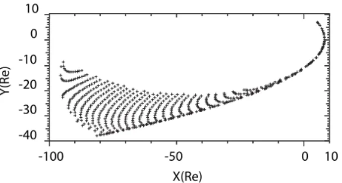
-100 0 10 -40 -30 -20 -10 0 10 X(Re) Y(Re) -50

Fig. 8. Points of intersection of the northern polar cap open field lines with the equatorial plane, shown by crosses.

-0.5 0 0.5 -0.5 0 0.5 80 70 60 Y(Re) X(Re) -0.5 0 0.5 -0.5 0 0.5 80 70 60 Y(Re) X(Re)

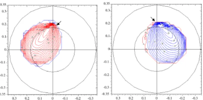
Fig. 9. Case 1. Left: The ionospheric electrostatic potential pat-terns in the northern polar cap are calculated at the time of case 1. The numbers denote the potential relative to the zero equipotential curves (which corresponds to the Sun-Earth line), with a contour separation of 16 kV. Only a single clockwise lobe cell shows up be-cause a second minor counterclockwise lobe is very small for this event IMF direction. The arrow marks the ionospheric projection of the cusp. Right: The ionospheric electrostatic potential patterns in the southern polar cap are calculated for the case 1. Potential drop between two lines is 16 kV. The solid circle shows the auroral oval boundary calculated for IMF=0. The equatorward boundary of the auroral oval corresponds to the inner edge of the tail current sheet. Only a single counterclockwise lobe cell shows up because a sec-ond minor clockwise lobe is very small for this event IMF direction. The arrow marks the ionospheric projection of the cusp.

The equipotentials located inside the regions bounded by the red and blue curves (Fig. 7) map to the convection lines of the polar caps. The open field lines that cross the magne-topause near the boundary marked by the red and blue curves in Fig. 7 map to the diffusion regions near the neutral points. The other open field lines, which intersect the magnetopause inside the open field line window, go far from the diffusion regions, and these field lines can be assumed to be equipo-tentials.

The small empty squares in Fig. 7 mark the positions of the magnetospheric cusps (magnetic field neutral points for IMF=0). For By>0, the northern (southern) cusp moves duskward (dawnward) and into the magnetosphere for Bz>0.

The potential drop between the neutral points, δ8sep, can be

estimated as (see Fig. 7)

δ8sep=8OS−8ON =2R1κEEIMFz, (7)

where 8OSand 8ON are electric potentials of the southern and northern neutral points, R1is the distance to the

subso-lar point of the magnetopause (R1=10RE, in the paraboloid model the distance along Z from the equatorial plane to the cusp is of the order of R1), EIMFz=By·V is the north-ward component of the interplanetary electric field, and κE describes the ratio of the ionospheric polar cap potential drop to the potential drop across the magnetosphere in the undisturbed solar wind (see Eq. 3). For both our events

κE=κBκv=0.05, where κV=0.5 was assumed. In this case, Eq. (7) gives δ8sep=0.1R1EIMFz.

The points of intersections of the northern polar cap open field lines bundle with the equatorial plane are shown by crosses in Fig. 8 (the solar magnetospheric coordinate sys-tem is used). The empty (without crosses) tailward region in Fig. 8 is crossed by closed (interconnected both hemi-spheres) tail lobe field lines. One may consider a part of these very long field lines as belonging to the polar cap be-cause they map to the dark polar ionosphere. We see that for this case, most of the northern open field lines cross the equatorial plane at the dawn side (at y<0). Only the lines nearest to the separator go to the dusk side near the subsolar equatorial plane. Almost all open field line bundles which cross- the equatorial plane are placed in the tail plasma sheet region. The nightside point of intersection of the separator with the equatorial plane is placed at X=−90 REand Y =−10 RE. The reconnection sites are projected to the boundary of the region covered by crosses. Open field lines appear at the sunward boundary of this region and then move in the an-tisunward direction and after intersecting with the tailward boundary transfer to the IMF lines.

Figure 9 shows the ionospheric electrostatic potential pat-terns in the northern and southern polar caps, respectively, calculated at the time of case 1. For case 2 the same po-lar cap potential patterns are shown in Fig. 10. The num-bers in Fig. 10 mark the distances along the electric field direction from the zero equipotential curve (which is cho-sen to coincide with the Sun-Earth line). These numbers are proportional to the corresponding potential values. The to-tal potential drop in the northern polar cap can be calculated by Eq. (6). The total magnetospheric size in the dawn-dusk direction is about 74 RE (see Fig. 8). In case 1 the pres-sure balance gives a subsolar distance R1=8.14 RE. The re-sults demonstrate that the size of one of the open field line windows Ly is 39RE, or about half of the total magneto-spheric size. In this case, Eq. (6) gives us 18npc=156 kV

for the northern polar cap, in good agreement with the re-sults of Blomberg et al. (2005), who studied two events il-lustrating the detailed relationships between plasma convec-tion, field-aligned currents, and polar auroral emissions, as well as illustrating the influence of the IMF By component

on theta aurora development. Electric and magnetic field and precipitating particle data are provided by DMSP, while the POLAR UVI instrument provides measurements of au-roral emissions. Ionospheric electrostatic potential patterns are calculated at different times during the evolution of the theta aurora using the KTH polar cap convection model. These model patterns have been compared to the convec-tion predicted by mapping the magnetopause electric field to the ionosphere using the paraboloid model of the mag-netosphere. The model results explain the correlation be-tween TPA occurrence and the By component of the IMF, because the potential drop on the separatrix is proportional to By. They support the observed TPA motion from dawn to dusk. In accordance with observations, the TPA region is collocated with sunward ionospheric convective flow.

For the field-aligned potential drop along the separator (between the neutral points), Eq. (7) gives 32 kV, a good agreement with the Siscoe et al. (2001) MHD simulations results. We can check our result by comparing with the po-lar cap potential drop which was determined by Korth et al. (2005). These authors presented a case study of a pro-longed interval of strongly northward IMF on 16 July 2000. Based on magnetic field observations by the constellation of Iridium satellites, together with the drift meter and magne-tometer observations from DMSP F13 and F15 satellites, and on the FUV images taken by the IMAGE spacecraft, Korth et al. (2005) estimated the electric potential drop as 45 kV. For the event interval (from 16:06 to 19:24 UT on 16 July 2000) the solar wind parameters were: Bt=6.76 nT, n=0.8 cm−3 and V =740 km/s (Korth et al., 2005), the total potential drop in the northern polar cap calculated by Eq. (6) is 53.49 kV, in good agreement with Korth et al. (2005). It is interest-ing to note that Korth et al. (2005) found that the potential drop associated with viscous interaction is less than ∼5 kV, or about 9 times smaller than the potential drop caused by high-latitude reconnection.

Figure 9 (right panel) shows the ionospheric electrostatic potential patterns in the southern polar cap calculated for case 1. The equipotentials are shown in blue and they cor-respond to the southern polar cap. The total potential drop in the southern polar cap is 128 kV. In Fig. 9 (right panel) the black solid circle, which corresponds to the auroral oval equatorial boundary, is shown for comparison. The equator-ward boundary of the auroral oval in our study corresponds to the inner edge of the tail current sheet.

We show in Figs. 9 and 10 only one convection cell. As a consequence of the method used here to calculate the con-vection lines, we can reproduce only the dominant lobe cell of a double lobe cell’s system. A minor convection cell which exists on the left (right) side of the clockwise (counter-clockwise) convection cell shown in the left panel of Fig. 9 and right panel of Fig. 10 (Fig. 9, right panel and 10, left panel) is not shown in these figures, since we would need a more complex calculation procedure for reproducing it. However, one should keep in the mind that really a two-cell

Fig. 10. Case 2. Left: Northern polar cap convection lines. Only a single clockwise lobe cell shows up because the second minor coun-terclockwise lobe is very small for this event IMF direction. The ar-row marks the ionospheric projection of the cusp. Right: Southern polar cap convection lines are shown. Only a single clockwise lobe cell shows up because the second minor counterclockwise lobe is very small for this event IMF direction. The arrow marks the iono-spheric projection of the cusp.

convection pattern with one cell much larger than the other exists in the open field line region in the polar cap for north-ward IMF with Bx6=0.

As one can see from Fig. 7 (bottom panel), for case 2 the transverse magnetospheric size Ly along the solar wind electric field direction is about 70 RE, in good agreement with the estimation 8R1=63.2 RE by Alexeev et al. (2000). Similar to case 1, the calculation results demonstrate that the size of one of the open field line windows is 40RE or about half of the total magnetospheric size. Finally, we have 18npc=157 kV for the northern polar cap and

18spc=150 kV for the southern polar cap. For the

field-aligned potential drop along the separator (between the neu-tral points), Eq. (7) gives 32 kV, which is the same as for case 1. The solar wind electric fields and subsolar distances are al-most equal for both these cases (ratio Esw1/Esw2is equal to 1.02, and R11/R12is equal to 1.03).

4 Summary

We studied here the modeled structure of the open field line bundles for northward IMF and forced solar wind conditions, which were observed during an event lasting several hours on 8 November 1998. Two cases, which were used for our analysis, correspond to opposite directions of the IMF By component.

Our results support the previous finding about a displace-ment of the ionospheric reconnection site projection (cusp) in the By (−By) direction for the northern (southern) polar cap (see, for example, Belenkaya, 1998b). The ionospheric open field line region shifts in the opposite direction. For the Northern Hemisphere our model predicts a convection change from a single clockwise lobe cell to a single coun-terclockwise lobe cell via an intermediate double lobe cell

system when the IMF changes from positive (case 1) to neg-ative IMF By (case 2) as during this event (in the 12:40– 15:30 UT period on this day).

We obtained estimates of the polar cap potential drops in both hemispheres. Model calculations showed that the north-ern and southnorth-ern potential drops can be different if Bx is comparable with By. If Bx<0, the potential drop is higher in the preferred northern polar cap, which is directly connected with the Sun by open field lines.

For northward IMF there are two connection points with the magnetosphere. In one cusp region, the IMF reconnects with closed field lines and forms open field lines, which are partially inside the magnetosphere and partially in interplan-etary space. In the other cusp region, open field lines of both polar caps form interplanetary and closed field lines.

For the southward IMF case, the northern and southern open field line windows at the magnetopause touch each other at the reconnection line (separator). The separator is placed in the magnetopause, inside the current sheet. Con-trary to it, for the northward IMF case, the northern and southern open field line windows at the magnetopause never touch each other. Between these windows the magnetopause is intersected by the IMF, which goes in and out of the magnetosphere. Inside the magnetosphere an IMF layer is formed.

Such a structure of the open field line bundles and the in-ner reconnection sites may explain why for the northward IMF the polar cap potential drop is about four times smaller than that for the southward IMF case, for the same value of the upstream solar wind electric field. We have demonstrated two reasons for the attenuation of the electric field inside the magnetosphere for northward IMF. First, the diameter of the open field line bundle is about half of the total size of the magnetosphere in the direction perpendicular to the electric field. The second reason for the reduction in the solar wind electric field inside the magnetosphere is the internal posi-tion of the reconnecposi-tion site. It is located at some distance inside the magnetosphere away from the magnetopause, and the flow velocity in this region is about half of the undis-turbed solar wind velocity.

Acknowledgements. We thank the ACE MAG and SWEPAM

in-strument teams and the ACE Science Center for providing the ACE data. The work at the Moscow State University was partially sup-ported by the RFBR Grants 05-05-64435, 06-05-64508, and 07-05-00529. Work at the Royal Institute of Technology was partially supported by the Swedish National Space Board and the Alfv´en Laboratory Centre for Space and Fusion Plasma Physics. Work at the University of Texas at Dallas was supported by NSF grant ATM0536868 and NASA grant NNG04GG84G.

Topical Editor I. A. Daglis thanks J. Dorelli and and another anonymous referee for their help in evaluating this paper.

References

Alexeev, I. I.: The penetration of interplanetary magnetic and elec-tric fields into the magnetosphere, J. Geomagn. Geoelectr., 38, 1199–1221, 1986.

Alexeev, I. I.: What define the polar cap and auroral oval diame-ter?, in: The Inner Magnetosphere: Physics and Modeling, edited by: Pulkkinen, T. I., Tsyganenko, N. A., and Friedel, R. H. W.: Geophysical Monograph Series, Volume 155, 313 pp., 257–262, ISBN 0-87590-420-3, AGU Code GM1554203, 2005.

Alekseyev, I. I. and Belenkaya, E. S.: Electric field in an open model of the magnetosphere, Geomagn. Aeron., Engl. Transl., 23, 57– 61, 1983.

Alexeev, I. I. and Belenkaya, E. S., Magnetospheric plasma con-vection on the open field lines, Geomagn. Aeron., 25, 450–457, 1985 (in Russian).

Alexeev, I.I. and Belenkaya, E. S.: Magnetospheric convection structure for the southward and northward IMF, Geomagn. Aeron., 29, 725–729, 1989 (in Russian).

Alexeev, I. I. and Kalegaev, V. V.: Magnetic field and the plasma flow structure near the magnetopause, J. Geophys. Res., 100(10), 19 267–19 276, 1995.

Alexeev, I. I., Belenkaya, E. S., and Clauer, C. R.: A model of re-gion 1 field-aligned currents dependent on ionospheric conduc-tivity and solar wind parameters, J. Geophys. Res., 105, 21 119– 21 127, 2000.

Alexeev, I. I., Sibeck, D. G., and Yu, S.: Bobrovnikov, Concerning the location of magnetopause merging as a function of the mag-netopause current strength, J. Geophys. Res., 103(A4), 6675– 6684, 1998.

Alexeev, I. I., Belenkaya, E. S., Bobrovnikov, S. Yu., and Kalegaev, V. V.: Modelling of the electromagnetic field in the interplanetary space and in the Earth’s magnetosphere, Space Sci. Rev., 107, 7– 26, 2003.

Belenkaya E. S.: Comment on “Observations of reconnection of interplanetary and lobe magnetic field lines at the high-latitude magnetopause” by Gosling, J. T., Thomsen, M. F., Bame, S. J., Elphic, R. C., and Russell, C. T., J. Geophys. Res., 98(A4), 5941–5944, 1993.

Belenkaya, E. S.: Reconnection modes for near-radial IMF, J. Geo-phys. Res., 103(A011), 26 487–26 494, 1998a.

Belenkaya, E. S.: High-latitude ionospheric convection patterns de-pendent on the variable IMF orientation, J. Atmos. Solar-Terr. Phys., 60/13, 1343–1354, 1998b.

Belenkaya, E. S., Alexeev, I. I., and Clauer, C. R.: Field-aligned current distribution in the transition current system, J. Geophys. Res., 109, A11207, doi:10.1029/2004JA010484, 2004.

Belenkaya E. S.: The Jovian magnetospheric magnetic and electric fields: effects of the interplanetary magnetic field, Planet. Space Sci., 52/5-6, 499–511, 2004.

Belenkaya, E. S., Cowley, S. W. H., and Alexeev, I. I.: Saturn’s aurora in the January 2004 events, Ann. Geophys., 24, 1649– 1663, 2006a.

Belenkaya, E. S., Bespalov, P. A., Davydenko, S. S., and Kalegaev, V. V.: Magnetic field influence on aurorae and the Jovian plasma disk radial structure, Ann. Geophys., 24, 973–988, 2006b. Blomberg, L. G., Cumnock, J. A., Alexeev, I. I., Belenkaya, E. S.,

Bobrovnikov, S. Yu., and Kalegaev, V. V.: Transpolar aurora: Time evolution, associated convection patterns, and a possible cause, Ann. Geophys., 23, 1917–1930, 2005,

http://www.ann-geophys.net/23/1917/2005/.

Bogdanova, Y. V., Marchaudon, A., Owen, C. J., Dunlop, M. W., Frey, H. U., Wild, J. A., Fazakerley, A. N., Klecker, B., Davies, J. A., and Milan, S. E.: On the formation of the high-altitude stagnant cusp: Cluster observations, Geophys. Res. Lett., 32, L12101, doi:10.1029/2005GL022813, 2005.

Carlson, H. C. and Cowley, S. W. H.: Accelerated polar rain elec-trons as the source of Sun-aligned arcs in the polar cap during northward interplanetary magnetic field conditions, J. Geophys. Res., 110, A05302, doi:10.1029/2004JA010669, 2005.

Cowley, S. W. H.: A qualitative study of the reconnection between the Earth’s magnetic field and an interplanetary field of arbitrary orientation, Radio Sci., 8(11), 903–913, 1973.

Cowley, S. W. H.: Interpretation of observed relations between solar-wind characteristics and effects at ionospheric altitudes, in: High Latitude Space Plasma Physics, edited by: Hultqvist, B. and Hagfors, T., 225–249, Plenum, New York, 1983.

Crooker, N. U.: Morphology of magnetic merging at the magne-topause, J. Atmos. Terr. Phys., 52, 1123–1134, 1990.

Crooker, N. U.: Reverse convection, J. Geophys. Res., 97, 19 363– 19 372, 1992.

Crooker, N. U., Siscoe, G. L., and Toffoletto, F. R.: A tangent sub-solar merging line, J. Geophys. Res., 95, 3787–3793, 1990. Crooker, N. U., Lyon, J. G., and Fedder, J. A.: MHD model merging

with IMF BY: Lobe cells, sunward polar cap convection, and overdraped lobes, J. Geophys. Res., 103, 9143–9151, 1998. Cumnock, J. A., Sharber, J. R., Heelis, R. A., Hairston, M. R.,

and Craven, J. D.: Evolution of the global aurora during posi-tive IMF Bz and varying IMF By conditions, J. Geophys. Res., 102, 17 489–17 498, 1997.

Cumnock, J. A. and Blomberg, L. G.: Transpolar arc evolution and associated potential patterns, Ann. Geophys., 22, 1213–1231, 2004,

http://www.ann-geophys.net/22/1213/2004/.

Cumnock, J. A.: High-latitude aurora during steady northward in-terplanetary magnetic field and changing IMF By, J. Geophys. Res., 110(A2), A02304, doi: 10.1029/2004JA010867, 2005. Cumnock, J. A., Blomberg, L. G., Alexeev, I. I., Belenkaya, E. S.,

Bobrovnikov, S. Yu., and Kalegaev, V. V.: Simultaneous polar aurorae and modelled convection patterns in both hemispheres, Adv. Space Res., 38, 1685–1693, 2006.

Dorelli, J. C., Hesse, M., Kuznetsova, M. M., Rastaetter, L., and Raeder, J.: A new look at driven magnetic reconnection at the ter-restrial subsolar magnetopause, J. Geophys. Res., 109, A12216, doi:10.1029/2004JA010458, 2004.

Dungey, J. W.: The structure of the exosphere or adventures in ve-locity space, in: Geophysics, The Earth’s Environment, edited by: DeWitt, C., Hieblot, J., and LeBeau, L., 503–550, Gordon and Breach, New York. 1963.

Frank, L. A., Craven, J. D., Burch, J. L., and Winningham, J. D.: Polar views of the Earth s aurora with Dynamics Explorer, Geo-phys. Res. Lett., 9, 1001–1004, 1982.

Frank, L. A., Craven, J. D., Gurnett, D. A., Shawhan, S. D., Weimer, D. R., Burch, J. L., Winningham, J. D., Chappell, C. R., Waite, J. H., Heelis, R. A., Maynard, N. C., Sugiura, M., Peterson, W. K., and Shelley, E. C.: The theta aurora, J. Geophys. Res., 91, 3177–3224, 1986.

Korth, H., Anderson, B. J., Frey, H. U., and Waters, C. L.: High-latitude electromagnetic and particle energy flux during an event with sustained strongly northward IMF, Ann. Geophys., 23, 1295–1310, 2005,

http://www.ann-geophys.net/23/1295/2005/.

Kullen, A., Brittnacher, M., Cumnock, J. A., and Blomberg, L. G.: Solar wind dependence of the occurrence and motion of polar auroral arcs: A statistical study, J. Geophys. Res., 107, 1362, doi:10.1029/2002JA009245, 2002.

Kullen, A. and Janhunen, P.: Relation of polar auroral arcs to mag-netotail twisting and IMF rotation: A systematic MHD simula-tion study, Ann. Geophys., 22, 951–970, 2004,

http://www.ann-geophys.net/22/951/2004/.

Lyons, L.: Generation of large-scale regions of auroral currents, electric potentials, and precipitation by the divergence of the con-vection electric field, J. Geophys. Res., 85, 17–25, 1980. Maynard, N. C., Burke, W. J., Moen, J., et al.: Responses of the

open – closed field line boundary in the evening sector to IMF changes: A source mechanism for Sun-aligned arcs, J. Geophys. Res., 108(A1), 1006, doi:10.1029/2001JA000174, 2003. Peterson, W. K. and Shelley, E. G.: Origin of the plasma in a cross

polar cap auroral feature (theta aurora), J. Geophys. Res., 89, 6729–6735, 1984.

Reiff, P. H. and Burch, J. L.: IMF By-dependent on dayside plasma flow and Birkeland currents in the dayside magnetosphere: 2. A global model for northward and southward IMF, J. Geophys. Res., 90, 1595–1611, 1985.

Siscoe, G. L.: The magnetospheric boundary, in Physics of Space Plasmas (1987), edited by: Chang, T., Crew, G. B., and Jasperse, J. R., 3–78, Sci. Publ., Inc., Cambridge, Mass., 1988.

Siscoe, G. L., Erickson, G. M., Sonnerup, B. U. ¨O., Maynard, N. C., Siebert, K. D., Weimer, D. R., and White, W. W.: Global role of Ek in magnetopause reconnection: An explicit demonstration, J. Geophys. Res., 106, 13 015–13 022, 2001.

Toffoletto, F. R. and Hill, T. W.: Mapping of the solar wind electric field to the Earth’s polar caps, J. Geophys. Res., 94(A1), 329– 347, 1989.

Vennerstrom, S., Moretto, T., Rastatter, L., and Raeder, J.: Field-aligned currents during northward interplanetary magnetic field: Morphology and causes, J. Geophys. Res., 110, A06205, doi:10.1029/2004JA010802, 2005.

Watanabe, M., Kabin, K., Sofko, G. J., Rankin, R., Gombosi, T. I., Ridley, A. J., and Clauer, C. R.: Internal reconnection for northward interplanetary magnetic field, J. Geophys. Res., 110, A06210, doi:10.1029/2004JA010832, 2005.

Yamamoto, T. and Ozaki, M.: A numerical model of the dayside aurora, J. Geophys. Res., 110, A05215, doi:10.1029/2004JA010786, 2005.