HAL Id: hal-00296062
https://hal.archives-ouvertes.fr/hal-00296062
Submitted on 23 Oct 2006
HAL is a multi-disciplinary open access
archive for the deposit and dissemination of
sci-entific research documents, whether they are
pub-lished or not. The documents may come from
teaching and research institutions in France or
abroad, or from public or private research centers.
L’archive ouverte pluridisciplinaire HAL, est
destinée au dépôt et à la diffusion de documents
scientifiques de niveau recherche, publiés ou non,
émanant des établissements d’enseignement et de
recherche français ou étrangers, des laboratoires
publics ou privés.
Longyearbyen, Svalbard
C. Vogler, S. Brönnimann, G. Hansen
To cite this version:
C. Vogler, S. Brönnimann, G. Hansen. Re-evaluation of the 1950?1962 total ozone record from
Longyearbyen, Svalbard. Atmospheric Chemistry and Physics, European Geosciences Union, 2006, 6
(12), pp.4763-4773. �hal-00296062�
www.atmos-chem-phys.net/6/4763/2006/ © Author(s) 2006. This work is licensed under a Creative Commons License.
Chemistry
and Physics
Re-evaluation of the 1950–1962 total ozone record from
Longyearbyen, Svalbard
C. Vogler1, S. Br¨onnimann1, and G. Hansen2
1Institute for Atmospheric and Climate Science, ETH Zurich, Switzerland 2Norwegian Institute for Air Research, Tromsø, Norway
Received: 9 December 2005 – Published in Atmos. Chem. Phys. Discuss.: 17 May 2006 Revised: 23 August 2006 – Accepted: 13 October 2006 – Published: 23 October 2006
Abstract. The historical total ozone measurements taken with Dobson Spectrophotometer #8 at Longyearbyen (78.2◦N, 15.6◦E), Svalbard, Norway, in the period 1950– 1962 have been re-analyzed and homogenized based on the original measurement logs, using present-day procedures. In lack of sufficient calibration information, an empirical quality assessment was performed, based on a climatolog-ical comparison with ozone measurements in Tromsø, us-ing TOMS data at both sites in the period 1979–2001, and ground-based Dobson data in the period 1950–1962. The as-sessment revealed that the C wavelength pair direct-sun (DS) measurements are most trustworthy (and most frequent), while the WMO standard reference mode AD direct-sun has a systematic bias. Zenith-blue (ZB) measurements at solar zenith angles (SZA) <78◦ were adjusted to DS data using different empirical functions before and after 1957 (the start of the International Geophysical Year). ZB measurements at larger SZAs were homogenized by means of a normalization function derived from days with measurements over a wide range of SZAs. Zenith-cloudy measurements, which are par-ticularly frequent during the summer months, were homoge-nized by applying correction factors depending on the cloud type (high thin clouds and medium to low thick clouds). The combination of all measurements yields a total of 4685 single values, covering 1637 days from September 1950 to Septem-ber 1962; moon measurements during the polar night add another 137 daily means. The re-evaluated data show a con-vincing consistence with measurements since 1979 (TOMS, SAOZ, Dobson) as well as with the 1957–1962 data stored at the World Ozone and UV Data Centre (WOUDC).
Correspondence to: G. Hansen ([email protected])
1 Introduction
Two decades after the discovery of the Antarctic ozone hole (Farman et al., 1985) and global ozone layer reduction, the chemical and dynamical processes causing ozone depletion are, to a large degree, understood and reproduced in chem-ical transport models (e.g., Chipperfield et al., 2005). An important tool to validate such models is to apply them to long time series of ozone and related stratospheric parame-ters, both in the “CFC” age and prior to it. This is also of great importance in order to make reliable predictions about the expected recovery of the ozone layer in the decades to come. For these reasons, much emphasis has been put into the re-evaluation of historical ozone data series during the last 10 years (Staehelin et al., 1998; Vanicek et al., 2003; Svendby, 2003; Hansen and Svenøe, 2005). At the same time, efforts have been taken to extend meteorological data records back in time, which can be used in order to inves-tigate the natural variability of the ozone layer in pre-CFC periods (Br¨onnimann, 2003; Br¨onnimann et al., 2004). The effect of dynamical processes on Arctic ozone and their rela-tion to large-scale climate variability are still not completely understood. There exist, however, only few total ozone series suitable for long-term studies, especially at high latitudes, where the largest natural and human-induced ozone varia-tions are observed.
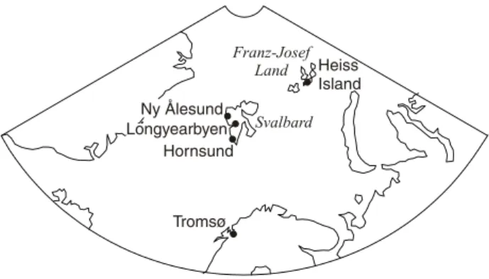
The measurements presented here started in Longyear-byen, Spitzbergen (the largest island of the Svalbard archipelago, see Fig. 1) in September 1950, after Dobson Spectrophotometer #8, which until then had been used for ozone measurements at the Norwegian sites Domb˚as and Oslo (Svendby, 2003), had undergone a major technical up-grade at Oxford. The instrument has been in use until to-day (including interruptions and relocations to Ny ˚Alesund in 1966–1968 and since 1995), but the earliest data have never
Fig. 1. Map showing the locations mentioned in the text.
been digitised. The purpose of this work was to re-evaluate the Longyearbyen total ozone data from 1950 to 1962 and to merge the new dataset with the data already stored in the World Ozone and UV Data Center (WOUDC), from the pe-riod 1957–1966 (and 1984–1993). This is the only data series poleward of 70◦prior to the International Geophysical Year (IGY) 1957/58. Thus, it can provide valuable information about the state of the Arctic ozone layer (natural variabil-ity, trends) before anthropogenic influences, e.g., CFC emis-sions, became noticeable. Combined with the recently re-evaluated ozone series from Tromsø, and the world’s longest ozone series from Arosa, Switzerland, it also yields a unique latitudinal chain of ozone measurements over almost two decades in the 1950s and 1960s.
In Sect. 2 of this paper, the measurement principle is out-lined. More details about the instrument history are given in Sect. 3, while the re-evaluation of the different measurement modes is discussed in the subsequent sections. The final data are shown in Sect. 8, followed by an outlook to future work.
2 Measurement principle
The first (electric) Dobson spectrophotometer was developed by Dobson around 1927 (Dobson, 1968) as a successor of the F´ery spectrophotograph, and manufacturing started in the late 1920s. In the 1940s and early 1950s, the instruments were re-constructed to allow measurements with additional wavelength combinations; moreover, they were equipped with photo-multipliers. For details about the early history of Dobson measurements see Dobson (1968). Although more modern methods, e.g., the Brewer technique and satellite measurements, are available today, Dobson AD direct-sun measurements are still WMO’s total ozone reference mea-surement mode, and Dobson meamea-surements are one of the few techniques which give satisfactory results under cloudy conditions using the so-called Zenith Cloud (ZC) method.
The measurement principle is to determine the intensity ratio of light at two wavelengths (wavelength pair) in the Huggins band of ozone absorption, one of which is strongly
absorbed by ozone, the other less so. Different wavelength pairs were in use, denoted A, B, C, C’, and D. C (combined with C’ under cloudy conditions) was the standard pair prior to the IGY 1957/58; since then the use of a dual wavelength pair (AD) was recommended in order to reduce interference from aerosol scattering. For the case of Longyearbyen, how-ever, the aerosol interference is expected to be only of mi-nor importance, except during episodes with severe volcanic aerosol loading (no major volcanic eruption occurred be-tween 1950 and 1962).
The light source can be direct sunlight (DS), light from the blue zenith (ZB), from the cloudy zenith (ZC), or moon-light. For the calculation of ozone values based on measure-ments using direct sunlight (DS) one needs the N -value (in-tensity ratio of the two wavelengths), the airmass (m, geo-metrical path length of the light through the atmosphere), µ (the ozone slant path, i.e., the length of the light path through the ozone layer), and the ozone absorption coefficients for the respective wavelengths. The N -value is obtained by conver-sion from the dial reading (R-value), which is the value read on the instrument. The conversion table is established and maintained for each wavelength pair separately by a calibra-tion of the transmission gradient of the optical wedge (wedge calibration) and by a comparison with a standard Dobson in-strument.
From measurements made at the zenith (ZB or ZC), ozone cannot directly be calculated. Instead, empirical relations have to be established, based on simultaneous DS measure-ments. For ZC observations, an additional wavelength pair (denoted C’) is used. Both wavelengths of this pair are only weakly absorbed by ozone, so that their ratio contains infor-mation about the wavelength dependence of the attenuation by clouds. Again, empirical methods have to be used to ob-tain ozone from these measurements.
Details about the instrument, the measurement techniques, the physical theory and the calculation of ozone values are given in, e.g., Dobson (1957), Komhyr (1980), Komhyr et al. (1993), Vanicek (2003) and Vanicek et al. (2003).
3 Instrument history and calculation of DS measure-ments
Ideally, detailed information about the instrument and the calibration history should be available for an accurate re-analysis. Necessary information is the raw data (R-values) and calibration information (at least R-N -conversion tables and standard lamp (SL) reference values including the his-tory of the SL-tests). An example of this kind of good prac-tice is found in Vanicek (2003) and Vanicek et al. (2003). In the original data sheets and documents of the 1950–1962 Longyearbyen data series, there is no information about the calibration of the instrument (despite an extra effort to find such information) so that a related statement would be spec-ulative. However, since the same instrument was used in
Domb˚as and Oslo in the period 1940–1949 (Svendby, 2003), one can state that the original registration and calculation forms prove that the observers showed great care in their work. All information about the instrument for the required period is from Langlo (1952) and Larsen (1959), which also served as source for Svendby (2003). In 1950, the Tromsø instrument (Dobson #14) was sent to Oxford for recalibra-tion and technical upgrading with a photomultiplier; it was returned to Norway together with Dobson #8 later the same year. This coincidence provides strong evidence that also #8 was re-calibrated and equipped with a photomultiplier before it was installed in Longyearbyen. During the first year, Søren H. H. Larsen was the responsible observer, fol-lowed by H. Welde, the superintendent of the coal mines at Longyearbyen.
Based on this information about the operators, the infor-mation in Svendby (2003) and the well-known contacts with G. M. B. Dobson in Oxford, we assume that the instrument was in good condition and was regularly checked for its sta-bility. It will be very challenging to recover additional infor-mation on the issue, after Søren H. H. Larsen passed away in the late 1990s. The only information in the original data are mercury lamp tests, standard lamp tests and wedge cali-bration tests for 1 July 1958, 1 November 1958, and 20 June 1959. In this period the instrument appears to have been sta-ble. However, the information from this short period does not allow to draw conclusions for the whole 13-year period of the re-analysis, but this is an indication that tests have been made regularly.
The original measuring protocols were available, contain-ing date, time, dial readcontain-ing (R-value) and weather informa-tion, as well as sheets on which the ozone values were cal-culated. A noticeable part of the work was the digitisation of the data, before they were ready for re-evaluation. Un-fortunately, we have no information about the original R-N conversion tables. Therefore, the conversion relation was de-rived by linear regression from the R- and N -values, for each wavelength pair separately, which are available in the origi-nal calculation protocols. These results were then applied to those R-values where no N -value was available. In the course of this procedure it became clear that the conversion must have changed between 1956 and 1957. For this reason we decided to apply two different conversions for the time before and after 1956/57. Although this is a purely empiri-cally motivated procedure, we regard it as the only reason-able way to handle the obvious change, which could have been caused by a wedge calibration.
At the time of the measurements the airmass and µ were calculated with the help of tables. Today this can be done more easily by computer programmes. In this study µ was calculated by the algorithm from Komhyr (1980), with an as-sumed ozone layer height of 18.2 km, while the airmass (m) is derived from Young (1994). The solar zenith angle (SZA), which is the basis for computing m and µ, was calculated by means of the LibRadtran scheme (Blanco-Muriel, 2001). For
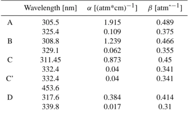
Table 1. Ozone absorption coefficients and Rayleigh scattering
co-efficients.
Wavelength [nm] α[(atm*cm)−1] β[atmˆ−1] A 305.5 1.915 0.489 325.4 0.109 0.375 B 308.8 1.239 0.466 329.1 0.062 0.355 C 311.45 0.873 0.45 332.4 0.04 0.341 C’ 332.4 0.04 0.341 453.6 D 317.6 0.384 0.414 339.8 0.017 0.31
this tool, only the exact date and time of the measurement, together with longitude and latitude, are needed.
The ozone absorption coefficients used in 1950 differ sig-nificantly from the ones used today. For this reason one has to use today’s standard coefficients (defined by WMO), see Komhyr et al. (1993). For a compilation of the used ozone absorption coefficients and Rayleigh scattering values see Table 1. For the derivation of ozone values x, the following equation was used:
x[DU]= 10 × N
(α−α0) × µ−1000 ×
(β−β0) × m ∗pp 0 (α−α0) × µ (single pair equation)
where α and β denote the absorption and scattering coeffi-cients (the prime denotes the longer wavelength of a pair), pis station pressure and p0is mean sea level pressure. As
mentioned in Sect. 2, aerosol scattering was neglected. In other total ozone re-analysis projects, e.g., Br¨onnimann et al. (2003), total ozone correction factors, based on the dif-ferent absorption coefficients at difdif-ferent times, were used to transfer ozone values from original values to updated values. The Longyearbyen original data from the 1950s and 1960s have never been published as a whole, but parts of it. At the World Ozone and UV Data Center (WOUDC) data base, data from 1957–1966 are stored, but compared to the original documents there are gaps, and a careful comparison revealed that the stored ozone data are sometimes based on less reli-able measuring modes. Sub-sets of the data were published by Larsen (1959), and the data were also compiled by the International Ozone Commission (archived at the UK Met Office, see Normand, 1961).
In all of these subsets of published data, there are uncer-tainties about which measuring modes were used for the cal-culation of the values, and none of these publications yields the same amount of information as the original data set re-analysed here. In order to use all information available to-day, including additional information in the original
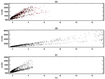
mea-Fig. 2. Ozone slant path as a function of ozone slant path
multi-plied by ozone value. Shown for the measuring modes DS, ZB and ZC. Black dots: Included measurements. Red dots: Excluded mea-surements. (Caution: The y-scale of the centre plot has a different scale).
surements protocols and more recent information on relia-bility of measurement modes and updated cross sections, we re-calculated the ozone values starting from the R readings.
In agreement with other ozone measurement series we first established a basic data set in the standard direct-sun (DS) mode based on the single wavelength pair C (as ex-plained in Sect. 4). For this data set, only measurements with µ<4.5 (solar zenith angle <∼78◦)were accepted. In
Wal-shaw (1975) G. M. B. Dobson describes that it is possible to extend the usable µ range of the C wavelength pair from 4 to 6 while using the focused image mode. Despite this option we chose 4.5 as an upper limit, as Fig. 2 (top plot) indicates that measurements with a higher µ are not reliable. Linearity of µ∗X versus µ is a good indicator of influence of the inter-nal scattered light on accuracy of total ozone observations. This method is included into the updated version of the Dob-son “Standard Operation Procedures” (SOPs) that are now being prepared by Bob Evans (Head of the World Dobson Calibration Center, NOAA, Boulder) as a WMO/GAW guide (K. Van´ıcek, personal communication).
The error resulting from day-to-day changes in station pressure is less than 0.5–1% even for high values of µ, total ozone and pressure variations, and is neglected for this rea-son. In addition, we rejected measurements that were flagged as unreliable on the observation sheets or showed obviously unrealistic values. As a result of this selection process, we were left with 1278 single measurements from 587 days. The distribution of the days of the year covered is mainly deter-mined by illumination conditions, which are sufficient ap-proximately from mid March until end of September, and by weather conditions, since DS observations require that the sun is not screened by clouds. However, also observer avail-ability and engagement seem to have played an important role for observation statistics.
4 Comparison with Tromsø total ozone in 1950–1962 and in TOMS data
Since there was no information available about the absolute calibration status of Dobson #8 in the time period investi-gated, a quality assessment of the Dobson total ozone record from Longyearbyen between 1950 and 1962 could only be made by an empirical quality check. For this purpose we as-sumed that the re-evaluated Tromsø series in the same time period could be used as a reference line. The distance be-tween the sites is about 800 km, but Tromsø is the only avail-able data series from high latitudes.
In order to establish a multi-annual (climatological) rela-tion between the Tromsø and the Longyearbyen series, we first compared the datasets from the TOMS instruments (Ver-sion 8) on board the satellites Nimbus-7, Meteor-3 and Earth Probe at the two sites. These data are available since 1979, with missing information for 1995 and 1996, when no TOMS instrument was operational. For Tromsø, data are available on almost all days from early February to early Novem-ber, while for Longyearbyen there are data only from early March until early October. Since we, in the historical dataset from Longyearbyen, have no direct-sun measurements be-fore March and after September, we made the comparison only for the period March-September. We also chose to limit the data to the time period 1979 until 2001, since the newest TOMS data, according to information at the TOMS home-page (http://toms.gsfc.nasa.gov/news/news.html, 18 Novem-ber 2004 news), suffer from degradation of the instrument with a latitude-dependent signature. As the measurement statistics of TOMS is very good for both sites, we calculated monthly means, from which we calculated monthly mean ra-tios xi=
Longyearbyeni
Tromsøi , (where i denotes the month) and used these values as reference ratios. As to be expected from geophysical conditions, the values for the early months, like March and April, turned out to have a larger variation than the summer and autumn months. The monthly mean ratios of the period March–May are slightly larger than 1, while the ratios in the other months are found to be between 0.94 and 1.00. The monthly ratios, averaged over the 23-year pe-riod are shown in Fig. 3 as a black curve (standard deviation: black dashed lines).
In a second step, similar ratios were derived for the (Dob-son) data from 1950–1962. However, since the data coverage is much poorer in the case of the Longyearbyen measure-ments (in contrast to Tromsø, where the coverage was very high in this period), we decided to calculate the ratio between Tromsø and Longyearbyen data on a daily basis and then to calculate monthly averages of the daily ratios.
Our approach assumes that the xi relation and its annual
course have remained constant since 1950, whereas the CFC-induced ozone depletion might not only affect mean ozone levels, but also the ratios xi due to the different distance of
Fig. 3. Ratios between Longyearbyen and Tromsø total ozone monthly means: TOMS 1979–2000 (black) with standard deviation (dashed lines), Longyearbyen Dobson 1950–1962 C-DS (red solid line), AD-DS (yellow), CD-DS (blue). Red dotted line: DS, ZB and ZC data on CC’ wavelengths. TOMS: ratios of monthly means at both sites; Longyearbyen Dobson: monthly means of ratios of daily means from both sites (reduced statistics).
Table 2. Availability of the different types of direct sun
measure-ments.
Single Daily means Years measurements
C-DS 1278 587 1950–1962 AD-DS 431 210 1951, 1957–1962 CD-DS 534 252 1951, 1957–1962
limitations, it should be noted that an effect is only expected in late winter and spring.
Before calculating ratios, we also raised the question about which DS wavelengths should be taken as a standard and base of comparisons. In principle, this question is answered by the number of available data in the different modes as given in Table 2.
According to WMO, the measurements at the AD wave-length pairs are the standard to which the other types need to be adjusted. However, in the case of the Longyearbyen mea-surements (as well as in the re-evaluated Tromsø series), AD is not the first choice for a standard data set due to the scarcity of measurements in this mode; from this aspect, the C direct sun measurements should be used as reference dataset.
A second – and more important – reason to take C direct sun measurements instead of AD as the reference data set, was the result of the Longyearbyen-Tromsø comparison as shown in Fig. 3. The annual variations of xi in all modes
are approximately the same as in the comparison based on TOMS data, except for September, when the statistics is much worse than in other months. However, both the AD DS
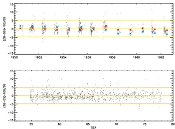
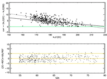
Fig. 4. Ratio between quasi-simultaneous zenith-blue and
direct-sun measurements sorted chronologically (upper panel) and as a function of solar zenith angle (lower panel). Annual means using one polynomial: blue asterisks, and using different polynomials be-fore and from 1957: red asterisks. Dots: single ratios based on two-function approach. Yellow lines: ±2 standard deviations.
(yellow curve) and the CD DS (blue curve) show a signif-icant negative bias relative to the TOMS references ratios, about 4% in the case of the AD mode and 10% in the case of the CD measurement mode. The C-mode derived values, on the other hand, agree with the TOMS reference ratios to within ±1 standard deviation in all months except August.
One could, of course, “normalise” the AD and the CD measurements empirically to the C measurements. However, this procedure would introduce further uncertainties, because the correlation between the different types is not very com-pact. Moreover, they would not add any new information to the total dataset; both AD and, trivially, CD measurements are only made on days when there are also C measurements, which are most reliable.
5 Zenith-blue (ZB) measurements
Zenith blue (ZB) observations use light scattered at the zenith during clear sky conditions instead of direct sun light. The calculation of ozone values for this measurement type is dif-ferent from the one for DS. It is not based on relationships that exactly describe physical processes, but it is calculated by establishing empirical relations between µ (or solar zenith angle, SZA) and N -value (derived from the dial reading) for ZB measurements and a reference ozone value from a quasi-simultaneous DS measurement (less than 15 min time offset). To establish this empirical relation we used a 3rd or-der polynomial function similar as in other studies (Svenøe, 2000; Vanicek et al., 2003):
O3ZB=a0+a1sza + a2N + a3sza2+a4N2+a5Nsza
Fig. 5. Ratio between direct-sun and zenith blue measurements on
days with measurements over a wide range of solar zenith angles: single values (black dots) and fit (red) used to normalise ZB mea-surements at SZA values >78◦. Blue dots: ZB data after normali-sation. Dotted line: Deviation of ±10%.
This regression model was calibrated using quasi-simultaneous DS measurements (from the C wavelength pair and µ<4.5; as described in Sects. 3 and 4), if available. The relative deviations of the residuals (O3,ZB-O3,DS)·100/O3,DS
are shown in Fig. 4. The yellow lines denote the mean and ±2 standard deviations. As one can see, the results are mostly within ±5%.
In a first approach, one polynomial was used for the whole dataset. But similar to the establishment of the R-N con-version, there seems to have been a shift between 1956 and 1957. In the upper plot of Fig. 4 the blue asterisks denote the mean value for every year, using this approach. By us-ing two different polynomial regressions (before and after 1957), a much better agreement with DS measurements can be achieved (red asterisks in Fig. 4).
The procedure was, in a second step, applied to all ZB measurements, also those without a quasi-simultaneous DS measurement, but only when solar zenith angles were less than 78◦(µ=4.5). At higher SZA values, the derived ozone values seemed to converge to a constant value, which is not realistic. Obviously, the polynomial was not suited for ex-trapolation.
Due to the geographical location of the site, there are, how-ever, a lot of ZB measurements with SZA values between 80◦and 96◦. These measurements were mostly made during
the early (late February, March) or late season (September– October), when there are no DS measurements. A utilisation of these measurements, if properly corrected, would add sig-nificantly to the data set as a whole. For this purpose we applied the same method as Svenøe (2000). The basic idea is to establish a relation between a reference DS value and ZB measurements at all SZA values up to 90 degrees on the same day. The pre-assumption is that the ozone value is
con-stant throughout the day, which is a very crude, but accept-able approach in lack of more detailed information. When comparing all ZB measurements (with varying SZA values) of the respective day with the reference DS value, one finds that this ratio for SZA>78◦is strongly dependent on SZA, as shown in Fig. 5 (black dots). The resulting ratio curve is then used to normalise the “high-SZA” measurements also in periods when no reference measurements with SZA<78◦ ex-ist. This procedure implies another assumption, namely that the normalisation function is not dependent on other factors, e.g. total ozone and ozone vertical distribution.
Most ZB measurements with high SZAs in Fig. 5 were made in 1950 and 1951. The occasional data from other years do not appear in the figure, because in these periods there were no DS reference measurements. To utilise these data we had to assume that the relationship for 1950 and 1951 is also valid for the other years. The correction function was limited to SZA<90◦, as the data scatter too much at larger SZAs due to worsening illumination conditions. We devel-oped the polynomial regression for 77◦<SZA<90◦and ap-plied it for 78◦<SZA<90◦(4.5<µ<13.3). The blue dots in Fig. 5 indicate the result of this correction. Most of the ZB values (SZA<78◦) are within ±5% (±2 standard deviations) of the DS reference values. From 78◦ to 90◦ the deviation is increasing up to a value of about ±10% (indicated by the dotted line). Thus a ZB value has an approximate maximum error of 10% at a SZA of 90◦.
By extending the upper limit for SZA to 90◦, but at the same time eliminating obviously erroneous outliers, 1482 single ozone values could be derived, from which 717 daily means were calculated. In Fig. 2 (middle panel) one can see that despite the extension of the µ-range up to 13 (SZA=90◦)
the obtained ozone values seem to be reliable (proven by the linearity). Note that for all panels in this figure there ap-pear to be two slopes, which is due to the seasonality of total ozone that is not fully sampled (missing mid-winter data). By including ZB data, more than 100 daily values were added to the 587 values available from the DS mode. These days are mostly found in the early or late months of the year when DS measurements are not possible.
6 Zenith-cloudy measurements
Under cloudy conditions the zenith-cloudy measurement mode (ZC) is applied. For this purpose, besides the C wave-length pair, one measures another pair, C’, which is close to the C wavelength pair. This second pair is used to correct the light extinction by clouds; for details see, e.g., Vanicek et al. (2003). The ZC measurements (more than 2500) can improve the data coverage considerably, as they are mostly taken on days without the possibility to take DS and ZB mea-surements. However, the treatment of ZC measurements is much more intricate, as it usually requires detailed weather information and information about cloud properties at a site.
During cloudy conditions, the N -value (derived from the dial reading) is too high compared to clear sky conditions, and one has to reduce it empirically to clear-sky values. This empirical correction, 1N , depends on cloud height and/or thickness, SZA and N C’ (the N -value from the second wavelength pair). It is calibrated using an ozone reference value for the same day from DS and/or ZB data. Again, the ozone value has to be assumed to be constant throughout the day. After the correction of the N -value further data process-ing is exactly the same as in the case of ZB.
For about 500 ZC measurements a reference (DS, ZB) value was available on the same day. The corrections turned out to be independent of SZA for values of up to 78◦(which is a logical consequence from the calibration of the ZB poly-nomial). For higher SZA there is a strong dependency. For this reason and due to the fact that there were not enough data for a satisfactory correction for high SZA, only ZC data with a SZA<78◦were considered. With these limitations, 392 ZC
measurements remained for the development of a cloud cor-rection. Further investigations showed that the correction is independent of the ozone column. Thus the remaining de-pendent variables are N C’ and cloud/weather information. The dependence of the correction on N C’ is shown in Fig. 6 (top panel, asterisks and diamonds).
The next step is to group the data according to differ-ent weather/cloud conditions. The most straightforward way is to classify into low (strong extinction), middle and high (weak extinction) clouds. This task is challenging, as the weather information was not systematic and with a highly varying degree of detail. More than 80% of the data in Fig. 6 (top panel) are characterized with the attributes “partly cloudy”, “overcast” or “light clouds”. The most frequent type is “partly cloudy”, which is diffuse but also has the largest probability of reference DS or ZB measurements.
Various tests using different classes of cloud characteris-tics finally resulted in the decision to make just two different groups of cloud types: high (light) clouds and middle & low clouds. From a linear least-square fit the following correction functions (see Fig. 6, top panel) were derived:
1N =22.291 − 0.099963 N C0
for high (light) clouds (solid line) 1N =37.334 − 0.17690 N C0
for middle and low clouds (dotted line)
These corrections were applied to all ZC measurements. In some cases, such as in autumn 1954, there was uncertainty about which group a measurement should belong to or there was no information about the clouds. In these cases the mean of the two corrections was applied. For some measurements between June and August 1956 the weather information in-dicated clear sky, which means that they can be considered as ZB measurements. Only very few of them, with a N C’ smaller than 200, have been corrected as above.
Fig. 6. Upper panel: Deviations of theoretical N -values between
reference daily means (from DS and ZB) and ZC N -values, as a function of ZC N (C’) values, sorted according to cloud characteris-tics: high/thin clouds (asterisks, linear fit: solid black line), middle and low clouds (diamonds, linear fit: dotted line). Lower panel: Comparison of ZC data and its daily reference value from DS/ZB (if available) as a function of SZA. Yellow lines: mean ±2 standard deviations.
Due to the empirical correction, ZC data inherently have a higher uncertainty than DS and ZB data. Assuming a mean correction for some measurements does not introduce more uncertainty than guessing a certain cloud type and using the corresponding correction.
The ZC data could then be processed in the same way as ZB data. Comparing the ZC data against the reference values (daily mean from DS and ZB) reveals a 2σ -error of ±5%. (see Fig. 6, lower panel). To this adds the uncertainty of the reference values themselves.
By including ZC data, 1925 single ozone values, corre-sponding to 1077 daily means, could be calculated and added to the dataset.
7 Moon measurements
This measuring mode is the only one which can provide data during the polar night (about 4 months in Longyearbyen), when the sun is not above the horizon at all. Only around full moon the light is sufficient for moon observations. A part of this data has already been published in 1959 (Larsen, 1959). It is well known that moon measurements are diffi-cult to perform and thus less reliable than day measurements. For this reason, overlap periods between moon and daylight measurements were used for quality assessment of the moon measurements, but only daylight measurements were used for daily means on these days. The measurement and the derivation of ozone values follow the same procedure as in the case of DS.
Fig. 7. Total ozone values from Longyearbyen Dobson in 1954:
Red diamonds: DS+ZB measurements; black asterisks: dataset in-cluding ZC mode.
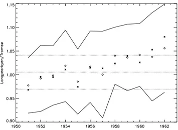
Fig. 8. Ratios of daily mean total ozone at Longyearbyen and
Tromsø, averaged from April to July in each year (asterisks: DS+ZB; diamonds: DS+ZB+ZC). The solid lines show ±1 stan-dard deviation for the diamonds (DS+ZB+ZC). The dashed lines represent the long-term mean (±1 standard deviation) of the ratio of April-to-July averaged total ozone at Longyearbyen and Tromsø based on TOMS data (1979–1989).
8 Final data set and quality check
The statistics for the daily mean values based on DS and ZB is given in Table 3 (DS only in parenthesis). It is obvious that the monthly measurement number distribution varies con-siderably from year to year. The years 1951–1955 have a rather good coverage from March to July, while in the years 1958–1960 only June and July contain a sufficient number of measurements; in 1961 and 1962 again the early months are covered best. This variation in the observation coverage is
Fig. 9. Total ozone monthly means for April (upper panel) and
July (lower panel): Bold solid line/squares: Dobson measurements at Longyearbyen (before 1994) and Ny- ˚Alesund (after 1994); thin solid line: TOMS data close to Ny- ˚Alesund; dashed line/diamonds (only April, since 1991): Ny- ˚Alesund DOAS; dotted line/triangles: Heiss Island M-83 (before 1990) and Brewer (after 1990).
mainly caused by weather conditions, but also the presence of operators may have played a role. The combination of DS and ZB data yields in total 2760 single ozone values, from which 817 daily means can be derived. If one adds the ZC data, (1925 single ozone values), one arrives at a total of 4685 single values covering 1637 days (Table 4). The doubling of daily means more than compensates the introduction of the larger single-value uncertainty, which is inherent to the ZC measurements. In fact, the inclusion of ZC measurements does not result in many more monthly means, but the num-ber of days per month is rising significantly. Figure 7 shows, as an example, all daily means for 1954. Red squares mark daily means from DS and ZB. On days with a black asterisk only the daily mean is solely based on ZC observations. If moon measurements are included, another 137 daily means can be added. The final data set of monthly means and num-ber of daily means per month are given in Table 5.
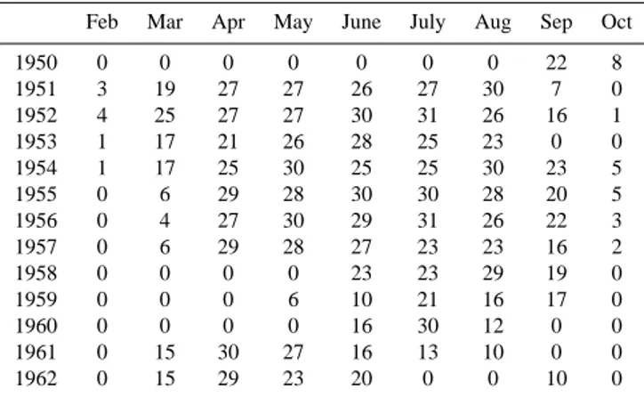
Table 3. Number of daily means for DS+ZB (DS).
Feb Mar Apr May June July Aug Sep Oct
1950 0 0 0 0 0 0 0 13 (8) 8 (0) 1951 3 (0) 19 (5) 22 (13) 18 (8) 10 (8) 13 (12) 9 (8) 1 (1) 0 1952 4 (0) 21 (3) 18 (18) 14 (14) 12 (12) 10 (9) 6 (4) 3 (1) 1 (0) 1953 1 (0) 17 (0) 14 (12) 17 (16) 11 (11) 18 (18) 5 (3) 0 0 1954 1 (0) 13 (0) 18 (18) 15 (13) 9 (9) 1 (0) 9 (0) 2 (0) 5 (0) 1955 0 6 (3) 17 (16) 22 (22) 21 (18) 4 (4) 7 (0) 8 (1) 5 (0) 1956 0 4 (4) 25 (20) 20 (14) 0 0 0 12 (3) 3 (0) 1957 0 6 (6) 20 (18) 15 (15) 9 (7) 5 (5) 5 (5) 5 (0) 2 (0) 1958 0 0 0 0 10 (10) 8 (7) 16 (13) 8 (5) 0 1959 0 0 0 2 (0) 6 (6) 13 (11) 8 (8) 9 (4) 0 1960 0 0 0 0 9 (9) 18 (16) 5 (3) 0 0 1961 0 12 (6) 27 (27) 17 (16) 5 (5) 0 0 0 0 1962 0 14 (8) 22 (22) 14 (14) 9 (9) 0 0 3 (3) 0
Table 4. Number of daily means for DS+ZB+ZC.
Feb Mar Apr May June July Aug Sep Oct
1950 0 0 0 0 0 0 0 22 8 1951 3 19 27 27 26 27 30 7 0 1952 4 25 27 27 30 31 26 16 1 1953 1 17 21 26 28 25 23 0 0 1954 1 17 25 30 25 25 30 23 5 1955 0 6 29 28 30 30 28 20 5 1956 0 4 27 30 29 31 26 22 3 1957 0 6 29 28 27 23 23 16 2 1958 0 0 0 0 23 23 29 19 0 1959 0 0 0 6 10 21 16 17 0 1960 0 0 0 0 16 30 12 0 0 1961 0 15 30 27 16 13 10 0 0 1962 0 15 29 23 20 0 0 10 0
Suspecting a change in the instrument set-up around 1956/57, we tested the homogeneity of the final data set. As in the initial quality check described in Sect. 4, this in-vestigation was based on a comparison between TOMS data and the re-analysed historical data, but now using the com-bination of DS, ZB and ZC measurements. The resulting Longyearbyen – Tromsø ratios are denoted by the dotted red line in Fig. 3. To investigate the stability of this parameter over time, the following procedure was applied: Ratios of daily mean values (DS+ZB) at Longyearbyen and Tromsø were averaged within each year over the period April to July. These were compared with means and standard deviations of the ratios of April-to-July averaged total ozone at Longyear-byen and Tromsø from TOMS data. As a reference period from TOMS we chose the period 1979–1989, during which only one TOMS instrument was in operation; in addition, stratospheric conditions were more stable than in the 1990s.
The results (Fig. 8) reveal that the ratio increases with time, but always remain well within the ±1σ range (dotted lines) of the TOMS-based reference ratios until 1960. If ZC data are included, the values are even closer to the reference, especially in 1961 and 1962. Taking into account the stan-dard deviations (solid lines) of the historical ratios, there is not sufficient statistical evidence for a change or a drift (note also that Tromsø data as well as data gaps contribute to the error). The trends found are in the order of about 2–3% over a 12-year period, which is not significant and maybe also ex-plainable with intermediate geophysical trends.
9 Outlook and conclusions
The re-evaluation of the historical Longyearbyen ozone data is the first, but most important step towards the establishment of a multi-decadal total ozone dataset for the European Arc-tic. More recent Dobson measurements from Svalbard are stored in the WOUDC database: Longyearbyen: from 1963 to 1966 and from 1984 to 1993; Ny ˚Alesund: from 1966 to 1968 and from 1995 to 1997 (the data since 1997 are under evaluation). While the data from the 1960s seem to agree well with the re-evaluated dataset (no obvious biases), there is more doubt about the measurements in the 1980s and early 1990s. These show significant (positive) biases relative to TOMS measurements from the same period.
In 1994, the instrument was moved to Ny- ˚Alesund, where measurements performed by staff from the Norwegian Po-lar Institute have continued until today. These data appear again more reliable and will be used, together with other ground-based and satellite measurements, to establish a more complete ozone data series from Svalbard. As a final step, it is envisaged to combine these data with further measure-ments from the region, e.g., Hornsund in the south of the archipelago and from Heiss Island in the Franz-Josef-Land
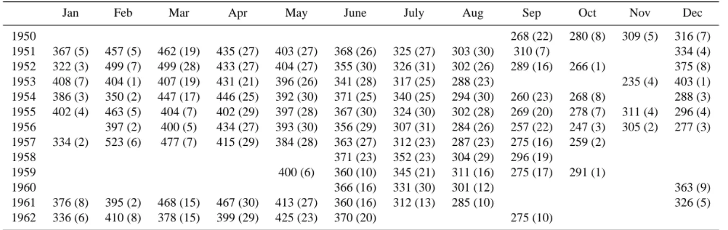
Table 5. Monthly total ozone means derived from the re-evaluated Longyearbyen Dobson measurements, including number of daily means
contributing to monthly means.
Jan Feb Mar Apr May June July Aug Sep Oct Nov Dec
1950 268 (22) 280 (8) 309 (5) 316 (7) 1951 367 (5) 457 (5) 462 (19) 435 (27) 403 (27) 368 (26) 325 (27) 303 (30) 310 (7) 334 (4) 1952 322 (3) 499 (7) 499 (28) 433 (27) 404 (27) 355 (30) 326 (31) 302 (26) 289 (16) 266 (1) 375 (8) 1953 408 (7) 404 (1) 407 (19) 431 (21) 396 (26) 341 (28) 317 (25) 288 (23) 235 (4) 403 (1) 1954 386 (3) 350 (2) 447 (17) 446 (25) 392 (30) 371 (25) 340 (25) 294 (30) 260 (23) 268 (8) 288 (3) 1955 402 (4) 463 (5) 404 (7) 402 (29) 397 (28) 367 (30) 324 (30) 302 (28) 269 (20) 278 (7) 311 (4) 296 (4) 1956 397 (2) 400 (5) 434 (27) 393 (30) 356 (29) 307 (31) 284 (26) 257 (22) 247 (3) 305 (2) 277 (3) 1957 334 (2) 523 (6) 477 (7) 415 (29) 384 (28) 363 (27) 312 (23) 287 (23) 275 (16) 259 (2) 1958 371 (23) 352 (23) 304 (29) 296 (19) 1959 400 (6) 360 (10) 345 (21) 311 (16) 275 (17) 291 (1) 1960 366 (16) 331 (30) 301 (12) 363 (9) 1961 376 (8) 395 (2) 468 (15) 467 (30) 413 (27) 360 (16) 312 (13) 285 (10) 326 (5) 1962 336 (6) 410 (8) 378 (15) 399 (29) 425 (23) 370 (20) 275 (10)
archipelago east of Svalbard into one European Arctic ozone series.
Figure 9 shows series of April and July monthly means comparing the Dobson measurements with both TOMS and DOAS (type SAOZ) at Svalbard (Longyearbyen and Ny
˚
Alesund), and measurements at Heiss Island. Obviously, the 1980s Dobson data are too high compared to TOMS, but the offset varies significantly with month. On the other hand, as to be expected from the validation procedure described in this work, the agreement between TOMS and the post-1994 Dobson data is good until about 2000, but also the agreement of the Dobson with the SAOZ data is convincing.
The Heiss Island Brewer data in the 1990s agree surpris-ingly well with the Svalbard TOMS and DOAS data, taking into account the distance between the sites, while the filter (M-83, M-129) data from the 1970s and 80s seem to have a non-negligible positive offset to Svalbard TOMS. Hence, be-fore the establishment of an Arctic ozone series these biases have to be investigated in more detail.
The final data set will be analysed by multi-linear regres-sion methods in a similar way as the Tromsø (Hansen and Svenøe, 2005) and the Arosa series (Appenzeller et al., 2000) in order to identify the parameters determining long-term variability of total ozone in the Arctic.
Acknowledgements. We thank the European Commission for
supporting this work in the frame of the CANDIDOZ project (EVK2-2001-00024) and the Swiss National Science Foundation for funding via the project “Past climate variability from an upper-level perspective”. The Norwegian Institute for Air Research (NILU) contributed with internal funding and infrastructure. The authors also thank Trond Svenøe, Norwegian Polar Institute, and Karel Vanicek, Czech Hydrometeorological Institute, for valuable discussions on the re-analysis of long-term historical data series.
Edited by: R. Volkamer
References
Appenzeller, C., Weiss, A. K., and Staehelin, J.: North Atlantic Os-cillation modulates Total Ozone Winter Trends, Geophys. Res. Lett., 27, 1131–1134, 2000.
Basher, R. E.: Review of the Dobson Spectrophotometer and Its Ac-curacy, WMO Global Ozone Research and Monitoring Project, Report No. 13, December 1982.
Blanco-Muriel, M., Blanco-Muriel, M., Alarcon-Padilla, D. C., Lopez-Moratalla, T., and Lara-Coira, M.: Computing the solar vector, Solar Energy, 70, 431–441, 2001.
Bojkov, R. D., Komhyr, W. D., Lapworth, A., and Vanicek, K.: Handbook for Dobson Ozone Data Re-evaluation, WMO/GAW Global Ozone Research and Monitoring Project, Report No. 29, WMO/TD-no. 597, 1993.
Br¨onnimann, S.: A historical upper-air data set for the 1939–1944 period, Int. J. Climatol., 23, 769–791, 2003.
Br¨onnimann, S., Cain, J. C., Staehelin, J., and Farmer, S. F. G.: Total ozone observations prior to the IGY. II. Data and quality, Q. J. R. Meteorol. Soc., 129, 2819–2843, 2003.
Br¨onnimann, S., Luterbacher, J., Staehelin, J., Svendby, T. M., Hansen, G., and Svenøe, T.: Extreme climate of the global tro-posphere and stratosphere in 1940–42 related to El Nino, Nature, 431, 971–974, 2004.
Chipperfield, M. P., Feng, W., and Rex, M.: Arctic ozone loss and climate sensitivity: Updated three-dimensional model study, Geophys. Res. Lett., 32, L11813, doi:10.1029/ 2005GL022674, 2005.
Dobson, G. M. B.: Observers’ handbook for the ozone spectropho-tometer, Ann. Int. Geophys. Year, Part 1, 5, 46–89, 1957. Dobson, G. M. B.: Forty years’ research on atmospheric ozone at
Oxford: A history, Appl. Opt., 7, 387–405, 1968.
Farman, J. C., Gardiner, B. G., and Shanklin, J. D.: Large losses of total ozone in Antarctica reveal seasonal ClOx/NOx interaction, Nature, 315, 207–210, 1985.
Hansen, G. and Svenøe, T.: Multilinear regression analysis of the 65-year Tromsø total ozone analysis, J. Geophys. Res., 110, D10103, doi:10.1029/2004JD005387, 2005.
Dobson Spectrophotometer, WMO Global Ozone Research and Monitoring Project, Report No. 6, 1980.
Komhyr, W. D., Mateer, C. L., and Hudson, R. D.: Effective Bass-Paur absorption coefficients for use with Dobson spectro-photometers, J. Geophys. Res., 98, 20 451–20 465, 1993. Langlo, K.: On the amount of atmospheric ozone and its relation to
meteorological conditions, Geofys. Publ., 18, No. 6, 5–44, 1952. Larsen, S. H. H.: Measurements of atmospheric ozone at Spitzber-gen (78N) and Troms¨o (70N) during the winter season, Geofys. Publ., 21, 5, 1–8, 1959.
Normand, C. W. B.: International Ozone Commission. Report of the Bureau for the years 1951–1954. 5 August 1954. In: Air Min-istry Branch, Ozone values (International Ozone Commission) (Unpublished Report MO 19/3/9 Part I (formerly MO 15/90) of UK MetOffice, 31 January 1961), 1954.
Staehelin, J., Renaud, A., Bader, J., McPeters, R., Viatte, P., Hoeg-ger, B., Bugnion, V., Giroud, M., and Schill, H.: Total ozone series at Arosa (Switzerland): Homogenization and data com-parison, J. Geophys. Res., 103, 5827–5841, 1998.
Svendby, T.: Reanalysis of total ozone measurements at Domb˚as and Oslo, Norway, from 1940 to 1949, J. Geophys. Res., 108(D24), 4750, doi:10.1029/2003JD003963, 2003.
Svenøe, T.: Re-evaluation, statistical analysis and prediction based on the Tromsø total ozone record, PhD Thesis, Faculty of Sci-ence, Department of Physics, The Auroral Observatory, Tromsø, October 2000.
Van´ıcek, K.: Calibration history of the Dobson 074 and Brewer 098 ozone spectro-photometers. Czech Hydrometeorol. Inst., Prague, ISBN 80-86690-08-3, 2003.
Van´ıcek K., Stanek M., and Dubrovsky, M.: Evaluation of Dobson and Brewer Total Ozone Observations from Hradec Kr´alov´e, Czech Republic, 1961–2002, Czech Hydrometeorol. Inst., Prague, ISBN 80-86690-10-5, 2003.
Walshaw, C. D (Ed.): Papers of Professor G. M. B. Dobson FRS, Publs. Inst. Geophys. Pol. Acad. Sci., 89, 61–115, 1975. Young, A. T.: Air mass and refraction, Appl. Opt., 33, 6, 1108–