HAL Id: hal-00345289
https://hal.archives-ouvertes.fr/hal-00345289
Submitted on 8 Dec 2008
HAL is a multi-disciplinary open access
archive for the deposit and dissemination of
sci-entific research documents, whether they are
pub-lished or not. The documents may come from
teaching and research institutions in France or
abroad, or from public or private research centers.
L’archive ouverte pluridisciplinaire HAL, est
destinée au dépôt et à la diffusion de documents
scientifiques de niveau recherche, publiés ou non,
émanant des établissements d’enseignement et de
recherche français ou étrangers, des laboratoires
publics ou privés.
Segmentation of Noisy Discrete Surfaces
Laurent Provot, Isabelle Debled-Rennesson
To cite this version:
Laurent Provot, Isabelle Debled-Rennesson. Segmentation of Noisy Discrete Surfaces. IWCIA 2008,
Apr 2008, Buffalo, NY, United States. pp.160-171, �10.1007/978-3-540-78275-9_14�. �hal-00345289�
Segmentation of Noisy Discrete Surfaces
?L. Provot and I. Debled-Rennesson
LORIA Nancy Campus Scientifique - BP 239 54506 Vandœuvre-l`es-Nancy Cedex, FRANCE
{provot, debled}@loria.fr
Abstract. We propose in this paper a segmentation process that can deal with noisy discrete objects. A flexible approach considering arith-metic discrete planes with a variable width is used to avoid the over-segmentation that might happen when classical over-segmentation algorithms based on regular discrete planes are used to decompose the surface of the object. A method to choose a seed and different segmentation strategies according to the shape of the surface are also proposed.
1
Introduction
Three-dimensional discrete objects are widely used in medical area. Due to their internal structure and their huge size, the manipulation of such objects is not an easy task. Rendering algorithms for instance, cannot apply usual techniques to obtain a nice visualization of the objects. A general idea to address this problem is to transform the discrete volume into a Euclidean polyhedra. The segmentation of the border of such objects into discrete primitives is thus a natural first step and several studies have been led on the subject.
In [6], L. Papier and J. Fran¸con propose a segmentation of the surface of a discrete object into pieces of standard arithmetic discrete planes. These standard planes are recognized using a Fourier-Motskin elimination algorithm [7] and are forced to be homeomorphic to a topological disk in order to be used in a polyhedrization process. They state that the resulting segmentation heavily depends on the choice of the seed to start the recognition of a new face and the tracking order of the points chosen for enlarging the current face, but do not address these problems.
In [2], J. Burguet and R. Malgouyres have developed a polyhedrization al-gorithm based on the computation of a topological Vorono¨ı diagram. Seeds are distributed on the surface of the discrete object according to its curvature [9] and a thinning algorithm is used to generate the skeleton of this surface without the seeds. The resulting Vorono¨ı regions can then be seen as a segmentation of the surface.
In the framework of surface area estimation [8], R. Klette and H.J. Sun have proposed a segmentation of the surface into digital planar segments (DPS) –
?
This work is supported by the ANR in the framework of the GEODIB project.
hal-00345289, version 1 - 8 Dec 2008
Author manuscript, published in "12th International Workshop on Combinatorial Image Analysis - IWCIA 2008, Buffalo, NY : United States (2008)" DOI : 10.1016/j.patcog.2008.11.032
which are actually pieces of standard discrete planes. To incrementally check whether a set of points is a DPS, they compute the convex hull of this set to retrieve a specific pair of parallel planes for which the main diagonal distance has to be less than √3. A breadth-first search of the surfel graph representing the surface is used to incrementally add points into the DPS.
In [13], I. Sivignon et al. have compared different tracking processes to de-compose the surface of a discrete object into naive discrete planes. A dual-space approach is used to incrementally recognize the pieces of planes [15]. In [14] the authors have also studied the relation between a segmentation into naive and standard discrete planes depending on the considered surface definition.
Although these methods are reversible and behave well with regular discrete objects, they might lead to an over-segmentation with noisy ones. In this paper we try to be more flexible and address the problem by considering a segmentation into pieces of discrete planes with a variable width. A first pre-processing step is done to compute geometric features of the surface of a possibly noisy discrete object. We then use these goemetric features to take into account the shape of the object to choose the seeds and to guide the incremental growth of the segments.
In section 2, after recalling the definition of blurred pieces of discrete planes, we summarize results from [11] about geometric features for noisy discrete sur-faces. The different steps of the segmentation process are then described in sec-tion 3, followed by some results on noisy and non-noisy objects. The paper ends up with a conclusion and some perspectives in section 4.
2
Background
We recall in this section the definition of a width-ν blurred piece of discrete plane, an arithmetical discrete primitive introduced in [10], that allows to deal with noisy discrete data. Relying on this primitive, we present the notion of a width-ν patch centered at a border point of a discrete objet and some features of the border obtained from this patch. More details about the construction of the patch and the study of different features of the border can be found in [11].
2.1 Blurred Pieces of Discrete Planes
One can see a blurred piece of discrete plane as an arithmetic discrete plane for which some points are missing. More formally:
Definition 1. Let N be a norm on R3
and E a set of points in Z3. We say that
the discrete plane P(a, b, c, µ, ω)1 is a bounding plane of E if all the points of
E belong to P, and we call width of P(a, b, c, µ, ω), the value ω−1 N (a,b,c).
A bounding plane of E is said optimal if its width is minimal.
1 An arithmetic discrete plane P(a, b, c, µ, ω) is the set of integer points (x, y, z)
veri-fying µ ≤ ax + by + cz < µ + ω, where (a, b, c) ∈ Z3is the normal vector of the plane. µ ∈ Z is named the translation constant and ω ∈ Z the arithmetical thickness.
Definition 2. A set E of points in Z3 is a width-ν blurred piece of discrete
plane if and only if the width of its optimal bounding plane is less than or equal to ν.
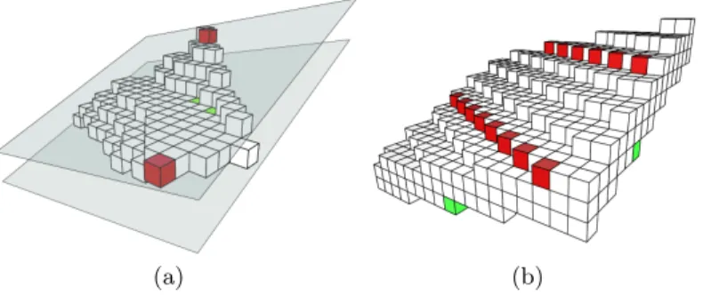
(a) (b)
Fig. 1. (a) A width-3 blurred piece of discrete plane and (b) a piece of its optimal bounding plane P(4, 8, 19, −80, 49), using the Euclidean norm.
Two recognition algorithms of blurred pieces of discrete planes have been proposed in [10]. The first one considers the Euclidean norm and, for a set of points P in Z3, it solves the recognition problem by using the geometry of the
convex hull of P . The second one considers the infinity norm and uses methods from linear programming to solve the recognition problem.
Thereafter, we denote by Ob a possibly noisy 6-connected discrete object.
We call surface or border of Obthe set of points Bb which have a 6-neighbor that
does not belong to Ob. All the results we present on this type of objects have
been obtained by considering the geometrical approach which uses the Euclidean norm.
2.2 Width-ν Discrete Patches
If we are working on a noisy discrete surface and need to extract some of its local geometric features, such as the normal vector or the curvature, it is wise to use estimators that take into account the irregularity of this surface to compute these kinds of features. A way to achieve this task at a point p of the surface is to gather the information of points lying in an extended neighborhood of p. The notion of patch we present hereafter takes place in this framework, considering an adaptative neighborhood around p.
Definition 3. Let Bb be the border of a discrete object, p a point in Bb and ν
the greatest real value allowed. Let d be a distance. At each point q ∈ Bb we
associate the weighting factor dp(q) = d(p, q). We call width-ν patch centered
at p, and denote by Γν(p), a width-ν blurred piece of discrete plane incrementally
recognized from p by adding points q of Bbfollowing the increasing values of dp(q).
About the Incremental Recognition: We construct a width-ν patch centered at p using the incremental recognition algorithm of blurred pieces of discrete planes introduced in [10]. We add the points following the increasing values of dp and, as soon as the width of the blurred piece of discrete plane becomes
greater than ν, we stop the recognition process.
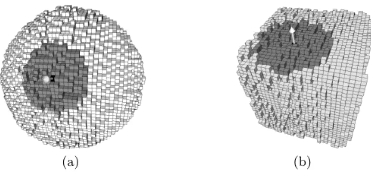
About the Distance d: To uniformly spread the patch in all directions, the best solution would be to use a geodesic distance. Nevertheless, for efficiency, we have chosen to rely on a distance based on a chamfer mask h3, 4, 5i which is a good approximation of the geodesic distance [1]. The aim is to have a well-balanced patch around p which looks almost circular. With this method we obtain patches like those in Fig. 2.
(a) (b)
Fig. 2. An example of width-2 patches spread on the surface of different noisy objects. (a) A sphere of radius 20 and (b) a cube of edge 25.
2.3 Patch Features
A patch Γν(p), as previously defined, characterizes the planarity of the surface
around p (with respect to the width ν). Thus, the more the patch is spread, the less the surface around p is bent.
In addition, if the growth of Γν(p) stopped, it means that the close
neigh-boring points outside Γν(p) would bend the patch too much if they were added.
In that case the patch could no longer be regarded as flat. Therefore, it is pos-sible to deduce a conformation of the discrete surface around p by studying the patches centered along the points of the outline of Γν(p).
The following definitions give a formal quantization of all these observations. Width-ν Normal With the previous intuition we can see that the normal vector of Γν(p) is a good estimation of the normal at p. Thus, assimilating the
normal vector of Γν(p) to the normal of the surface at p, we define a normal
vector estimator for each point of the surface of a possibly noisy discrete object.
Definition 4. Let Bb be the border of a discrete object and p a point of Bb. We
call width-ν normal at p the normal vector −→
nν(p) = −→n (Γν(p))
where −→n (Γν(p)) is the normal vector of the patch Γν(p).
Width-ν Patch Area Given a Euclidean surface S and its normal vector field {−→n }, in the continuous space we can compute the area of S with the formula:
A(S) = Z
S
− →n (s) ds
The discrete version of this equation given in [4] has been adapted as follows to compute the area of the surface of a width-ν patch:
EA(Γν(p)) = X s∈SΓν (p) −→ nν(p).−→nel(s) = −n→ν(p). X s∈SΓν (p) − →n el(s)
where SΓν(p)is the set of surfels
2of the patch surface, and −→n
el(s) the elementary
normal vector of s.
Shape Estimator An estimator that enables the characterization of the shape (concave, convex or flat) of the surface around a border point of a possibly noisy discrete object has been developed. It is based on the study of the conformation of the patches which are centered on points belonging to the outline of Γν(p).
Definition 5 (Patch Outline). Let Bb be the border of a discrete object Ob.
We denote by Sb the set of surfels of Bb which are incident to a point that does
not belong to Ob, and SΓν(p) the subset of Sb that belongs to Γν(p). A point q belongs to the outline of Γν(p) if the voxel representation of q has a surfel
s ∈ SΓν(p) and if there exists a surfel s
0 ∈ S
b \ SΓν(p) such that s and s 0 are
adjacent by edge.
Let C be the set of points that belong to the outline of Γν(p). Our shape
estimator of the surface around a point p is then given by the formula : Fν(p) = 1 |C| X ∀q∈C \ (−n→ν(p), −n→ν(q)) · EA(Γν(q)) EA(Γν(p))
where(−n→ν(p), −\n→ν(q)) is the oriented angle value between the two normal vectors. So, the estimator Fν(p) is a weighted mean of the angle values between −n→ν(p)
and the −n→ν(qi)1≤i≤|C|.
2
Faces of a voxel are called surfels
Fν(p) is positive when the surface around p is rather convex and Fν(p) is
negative when the surface around p is rather concave. An increasing value of |Fν(p)| means that the surface around p is more strongly concave or convex.
Moreover, if Γν(p) is big, a value Fν(p) close to zero means that the area around
p is almost flat (according to the width ν we chose). If Γν(p) is small, then the
area around p is strongly distorted, but in a way we can neither qualify concave, nor qualify convex (a saddle point for instance).
3
Segmentation
3.1 Introduction
The segmentation of a tridimensional discrete object we will describe in this section consists in partitioning the border of the object into pieces of discrete planes. Some studies have been led on the subject [8, 13, 14, 2, 6] but they all consider regular planes with a fixed width (mainly naive or standard arithmetic discrete planes). Although these methods give good results with regular discrete objects (Fig. 3(a)), it is not always the case when we have to deal with irregular or noisy discrete objects (Fig. 3(b)). In particular, irregularities force to create lots of small segments. The approach we present hereafter is more flexible and considers a segmentation into pieces of planes with a variable width, width-ν blurred pieces of discrete planes (denoted BP DPν in the sequel) to be specific,
to deal with noisy data.
(a) (b)
Fig. 3. Segmentation of (a) a regular cube of edge 25 and (b) a noisy counterpart by using the DSD algorithm (http://liris.cnrs.fr/isabelle.sivignon/DSD.html) proposed by I. Sivignon [13, 14].
3.2 Segmentation into Blurred Pieces of Discrete Planes
Firstly, a pre-processing step is done on the borber Bb of the discrete object we
want to segment. Given a real ν, for each point p ∈ Bb we compute a width-ν
patch centered at p as explained in section 2.2. At each point p we can thus associate the features presented in section 2.3, that is:
– the normal vector −n→ν(p),
– the area factor EA(Γν(p)),
– and the shape factor Fν(p).
Our segmentation process can be summed up to the following steps: a seed is chosen among points of Bbto start a first BP DPν recognition that grows through
a process of accretion. An adjacent point is selected and added to BP DPν if it
satisfies some required criteria. The BP DPνeventually stops growing when there
are no more adjacent points that can be added without contradicting the crite-ria. This procedure is repeated from a new seed until all points of Bb belong to
a BP DPν.
In the following paragraphs we will discuss more in details the different key points of this segmentation algorithm.
Seed Selection. The easiest way to choose a seed is to randomly pick a border point which does not belong to a BP DPν and to start the recognition process
from there. The problem with this approach is that we have no control over the segmentation. To segment a cube for instance, a bad choice would be to start from seeds that lie near an edge of the cube. This would result in an over-segmentation as shown in Fig 4.
A better choice is to start from seeds that are lying in flat areas. It is indeed more meaningful to give a higher priority to flat areas than to bent areas since the underlying primitive of a BP DPν is an arithmetical discrete plane. Chances
to have a better approximation are thus higher. Therefore we have chosen to rely on the area estimator EA(Γν(p)) to find the seeds. The idea is to pick the
border point p (not yet processed) which has the highest EA(Γν(p)) value as the
next seed.
BP DPν Recognition. The algorithm used to incrementally recognize
width-ν blurred pieces of discrete planes is the geometrical one proposed in [10] by considering the Euclidean norm.
The spreading of a BP DPν heavily depends on the way the neighborhood of
the seed is visited as explained in [13]. For the same reasons as before, the value EA(Γν(p)) is used in the accretion process. Points p adjacent to the evolving
BP DPν are added according to their decreasing EA(Γν(p)) values.
To implement this behaviour we use a priority queue Q. We start by pushing the seed into the queue with a weight equals to its area factor and mark this seed as visited. Then, while Q is not empty, we pop out of Q the point p with the highest weight w and we add p to the evolving BP DPν if it satisfies the
requiered criteria presented in the following paragraph. We then add the non-visited 26-neighbours of p which belong to the border and their associated area factor into the priority queue Q and mark them as visited.
Using this technique the BP DPν does not stop growing if a point cannot be
added.
Fig. 4. Over-segmentation due to randomly chosen seeds.
(a)
(b) (c) (d)
Fig. 5. The points that belong to the BP DPνare
in grey (a) Processing order of the neighborhood. (b-d) Some possible configurations when we try to add the point with the question mark: (b) it cannot be added because it is not 4-connected to another grey point; (c) it cannot be added because it creates a hole; and (d) it can be added.
Required Criteria. The first criterion that has to be satisfied is that the width of the evolving BP DPν must not exceed ν when a point p is added. But this is
implicitly checked in the recognition algorithm.
Moreover, as we plan to use the segmentation in a future work to develop a polyhedrization algorithm for noisy discrete objects, the BP DPν segments have
to satisfy some constraints of good formation. In particular we want a BP DPν
segment to be 4-connected and without holes, i.e. homeomorphic to a topolog-ical disk, according to the main direction of the normal vector of its seed. To check these constraints we use a simplified version of a method proposed in [12] (p.153). We work in the projection plane associated to the normal vector of the seed. We consider the 8-neighborhood of the point we are trying to add in the evolving BP DPν and process the 8-neighbors in the order shown in Fig. 5(a).
During the processing a zero-initialized counter is incremented at each time we go from a point which belongs to BP DPν to a point which does not, and
vice-versa. At the end, if the counter value is greater than two it means that the point cannot be added whitout creating a hole. In the same time we check that at least one 4-neighbor belongs to BP DPν. If a point does not pass these checks
it is marked as non-visited to give the tracking process the opportunity to visit it later on.
Some results obtained with this segmentation method are given in Fig. 6(a) and 6(b). On the one hand, if we look at the cube in Fig. 6(a), we can see that the segmentation is rather good and partition the object into six segments which correspond to the six faces of the cube. On the other hand, the segmentation of the sphere in Fig. 6(b) could be better. The problem with the sphere is its curved border. The tracking process of points described in section 3.2 has the
opportunity to skirt round the points that cannot be added and on curved parts it tends to create rough-crescent-shaped BP DPν. If we now use a width-ν
patch-based segmentation, as described in section 2.2, we can see that the result is far better (see Fig. 6(c)). This is due to the chamfer-mask-based tracking process used to grow the patches.
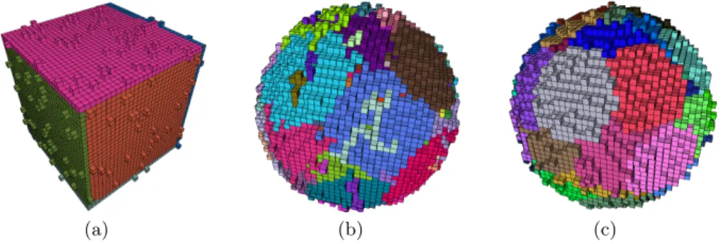
(a) (b) (c)
Fig. 6. Width-2 segmentation of a weakly (a) noisy cube of edge 30; (b) noisy sphere of radius 20 with the method presented in section 3.2. (c) Segmentation of the same sphere using only width-2 patches.
3.3 Hybrid Method
Relying on the previous observations, we have developed an hybrid segmentation method. For seeds that lie in a flat part of the object we develop a BP DPν
segment as described in 3.2 and for seeds that lie in curved parts we develop a patch Γν(p) (see section 2.2).
To distinguish between flat parts and curved parts we use the shape factor Fν(p). As previously explained, an increasing value of |Fν(p)| means that the
surface around p is more strongly bent. Thus, given a threshold value σ and a seed s, if |Fν(s)| < σ we develop a BP DPν segment, otherwise we develop a
patch Γν(s).
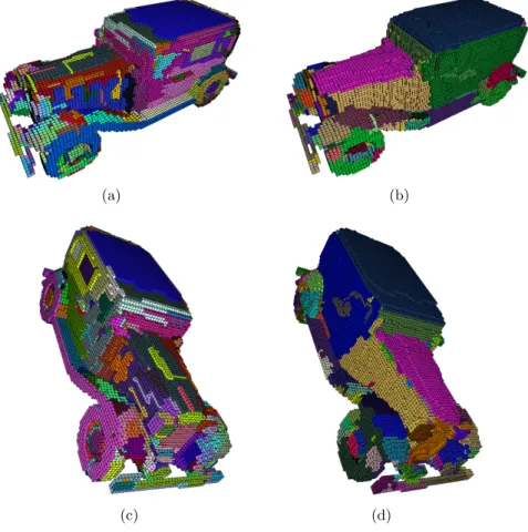
Results obtained with this method are shown in Fig. 7 and 8. In Fig. 7 synthetical objects with different shapes have been segmented at different widths. We can see in Fig. 7(g) and 7(h) that the method still works for non-noisy objects. Furthermore, due to the hybrid approach, both the flat and the curved areas of the noisy half hallowed ellipsoid in Fig 7(c), 7(f) and 7(i), are well segemented. In Fig. 8 a real-life object – an old Dodge car, available on the TC18 website3
– has been segmented with both, the DSD algorithm proposed by I. Sivignon and the hybrid approach. We can notice that, with the hybrid approach, the flat
3
http://www.cb.uu.se/~tc18/code_data_set/3D_images.html
areas, i.e the roof, the parts of the hood and the windshield, are well segmented, with respect to the shape of the car and with a little number of segments. In curved areas the two segmentations are close, but it is difficult to decide what is a “good” segmentation in these areas.
(a) (b) (c)
(d) (e) (f)
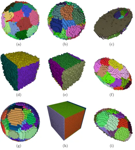
(g) (h) (i)
Fig. 7. Results of different segmentations by using the hybrid method on synthetical objects: (a, b) a width-2 segmentation of a weakly noisy sphere of radius 20; (d, e) a width-3 segmentation of a strongly noisy cube of edge 25; (g, h) a width-1 segmentation of non-noisy objects; and (c, f, i) a width-2 segmentation of an half hallowed ellipsoid.
Note that, at this time, the threshold have to be set manualy, but we would like to investigate more to find a way to automaticaly choose a good value for σ.
4
Conclusion
In this paper we have presented a segmentation method to decompose a possibly noisy discrete object into pieces of discrete planes with a variable width. Different segmentation strategies have been proposed, guided by geometric features of the border of the object, computed in a pre-process step. Good results have been obtained for both noisy and non-noisy objects, but we still have to investigate more to automaticaly choose good values for the different parameters of the method.
(a) (b)
(c) (d)
Fig. 8. The segmentation of a car (a, c) by using the DSD algorithm of I. Sivignon; and (b, d) by using the width-2 hybrid method.
In a future work, we intend to use this segmentation to develop a smoothing and a polyhedrization algorithms for noisy discrete objects. But some work have to be done to propose a good definition for facets and to study the way to group
them together to build a Euclidean polyhedron. The strategies used in [5] and in [3] could help us in that way. We also intend to lead formal studies on the notion of noise to give a theoretical validation of the presented approach.
References
1. Borgefors, G.: On digital distance transforms in three dimensions. Computer Vision and Image Understanding 64(3) (1996) 368–376
2. Burguet, J., Malgouyres, R.: Strong thinning and polyhedrization of the surface of a voxel object. In: 9th International Conference on Discrete Geometry for Computer Imagery. Volume 1953 of LNCS., Uppsala, Sweden (2000) 222–234
3. Coeurjolly, D., Dupont, F., Jospin, L., Sivignon, I.: Optimization schemes for the reversible discrete volume polyhedrization using marching cubes simplification. In: 13th International Conference on Discrete Geometry for Computer Imagery. Volume 4245 of LNCS., Szeged, Hungary (2006) 413–424
4. Coeurjolly, D., Flin, F., Teytaud, O., Tougne, L.: Multigrid convergence and sur-face area estimation. In: Theoretical Foundations of Computer Vision “Geometry, Morphology, and Computational Imaging”. Volume 2616 of LNCS. (2003) 101–119 5. Dexet, M., Coeurjolly, D., Andres, E.: Invertible polygonalization of 3d planar digital curves and application to volume data reconstruction. In: 2nd International Symposium on Visual Computing. Volume 4292 of LNCS., Lake Tahoe, Nevada, USA (2006) 514–523
6. Fran¸con, J., Papier, L.: Polyhedrization of the boundary of a voxel object. In: 8th International Conference on Discrete Geometry for Computer Imagery. Volume 1568 of LNCS., Marne-la-Vallee, France (1999) 425–434
7. Fran¸con, J., Schramm, J.M., Tajine, M.: Recognizing arithmetic straight lines and planes. In: 6th International Workshop on Discrete Geometry for Computer Imagery. Volume 1176 of LNCS., Lyon, France (1996) 141–150
8. Klette, R., Sun, H.J.: Digital planar segment based polyhedrization for surface area estimation. In: 4th International Workshop on Visual Form. Volume 2059 of LNCS., Capri, Italy (2001) 356–366
9. Lenoir, A.: Fast estimation of mean curvature on the surface of a 3d discrete ob-ject. In: 7th International Workshop on Discrete Geometry for Computer Imagery. Volume 1347 of LNCS., Montpellier, France (1997) 175–186
10. Provot, L., Buzer, L., Debled-Rennesson, I.: Recognition of blurred pieces of dis-crete planes. In: 13th International Conference on Disdis-crete Geometry for Computer Imagery. Volume 4245 of LNCS., Szeged, Hungary (2006) 65–76
11. Provot, L., Debled-Rennesson, I.: Geometric feature estimators for noisy dis-crete surfaces. Technical report, Loria (2007) http://www.loria.fr/~provot/ doc/geom_feature_estimators.pdf.
12. Sivignon, I.: De la caract´erisation des primitives `a la reconstruction poly´edrique de surfaces en g´eom´etrie discr`ete. Th`ese, I.N.P. de Grenoble (2004)
13. Sivignon, I., Dupont, F., Chassery, J.M.: Decomposition of a three-dimensional discrete object surface into discrete plane pieces. Algorithmica 38(1) (2004) 25–43 14. Sivignon, I., Dupont, F., Chassery, J.M.: Discrete surface segmentation into dis-crete planes. In: 10th International Workshop on Combinatorial Image Analysis. Volume 3322 of LNCS., Auckland, New Zealand (2004) 458–473
15. Vittone, J., Chassery, J.M.: Recognition of digital naive planes and polyhedriza-tion. In: 9th International Conference on Discrete Geometry for Computer Imagery. Volume 1953 of LNCS., Uppsala, Sweden (2000) 296–307