HAL Id: hal-00761611
https://hal.archives-ouvertes.fr/hal-00761611
Submitted on 5 Dec 2012HAL is a multi-disciplinary open access
archive for the deposit and dissemination of sci-entific research documents, whether they are pub-lished or not. The documents may come from teaching and research institutions in France or abroad, or from public or private research centers.
L’archive ouverte pluridisciplinaire HAL, est destinée au dépôt et à la diffusion de documents scientifiques de niveau recherche, publiés ou non, émanant des établissements d’enseignement et de recherche français ou étrangers, des laboratoires publics ou privés.
Andrés Aristizábal, Filippo Bonchi, Luis Pino, Frank D. Valencia
To cite this version:
Andrés Aristizábal, Filippo Bonchi, Luis Pino, Frank D. Valencia. Reducing Weak to Strong Bisimi-larity in CCP. Fifth Interaction and Concurrency Experience, Jun 2012, Stockholm, Sweden. pp.2-16, �10.4204/EPTCS.104�. �hal-00761611�
Andr´es Aristiz´abal
CNRS/DGA and LIX ´Ecole Polytechnique de Paris
Filippo Bonchi
ENS Lyon, Universit´e de Lyon, LIP (UMR 5668 CNRS ENS Lyon UCBL INRIA), 46 All´ee d’Italie, 69364 Lyon, France
Luis Pino
INRIA/DGA and LIX ´Ecole Polytechnique de Paris
Frank Valencia
CNRS and LIX ´Ecole Polytechnique de Paris
Concurrent constraint programming (ccp) is a well-established model for concurrency that singles out the fundamental aspects of asynchronous systems whose agents (or processes) evolve by post-ing and querypost-ing (partial) information in a global medium. Bisimilarity is a standard behavioural equivalence in concurrency theory. However, only recently a well-behaved notion of bisimilarity for ccp, and a ccp partition refinement algorithm for deciding the strong version of this equivalence have been proposed. Weak bisimiliarity is a central behavioural equivalence in process calculi and it is ob-tained from the strong case by taking into account only the actions that are observable in the system. Typically, the standard partition refinement can also be used for deciding weak bisimilarity simply by using Milner’s reduction from weak to strong bisimilarity; a technique referred to as saturation. In this paper we demonstrate that, because of its involved labeled transitions, the above-mentioned saturation technique does not work for ccp. We give an alternative reduction from weak ccp bisimi-larity to the strong one that allows us to use the ccp partition refinement algorithm for deciding this equivalence.
1
Introduction
Since the introduction of process calculi, one of the richest sources of foundational investigations stemmed from the analysis of behavioural equivalences: in any formal process language, systems which are syn-tactically different may denote the same process, i.e., they have the same observable behaviour.
A major dichotomy among behavioural equivalences concerns strong and weak equivalences. In strong equivalences, all the transitions performed by a system are deemed observable. In weak equiv-alences, instead, internal transitions (usually denoted by τ) are unobservable. On the one hand, weak equivalences are more abstract (and thus closer to the intuitive notion of behaviour); on the other hand, strong equivalences are usually much easier to be checked (for instance, in [17] a strong equivalence is introduced which is computable for a Turing complete formalism).
Strong bisimilarity is one of the most studied behavioural equivalence and many algorithms (e.g., [30, 11, 12]) have been developed to check whether two systems are equivalent up to strong bisimilarity. Among these, the partition refinement algorithm [15] is one of the best known: first it generates the state
∗This work has been partially supported by the project ANR-09-BLAN-0169-01 PANDA, and by the French Defence
space of a labeled transition system (LTS), i.e., the set of states reachable through the transitions; then, it creates a partition equating all states and afterwards, iteratively, refines these partitions by splitting non equivalent states. At the end, the resulting partition equates all and only bisimilar states.
Weak bisimilaritycan be computed by reducing it to strong bisimilarity. Given an LTS−→ labeled· with actions a, b, . . . one can build=⇒ as follows.·
P−→ Qa P=⇒ Qa P=⇒ Pτ P=⇒ Pτ 1 a =⇒ Q1 τ =⇒ Q P=⇒ Qa
Since weak bisimilarity on−→ coincides with strong bisimilarity ona =⇒, then one can check weaka bisimilarity with the algorithms for strong bisimilarity on the new LTS=⇒.a
It is worth pointing out that an alternative presentation of=⇒ with sequences of actions as labels is· also possible [19]. Nevertheless, the resulting transition system may be infinite-branching and hence not amenable to automatic verification using standard algorithms such as partition refinement.
Concurrent Constraint Programming(ccp) [26] is a formalism that combines the traditional algebraic and operational view of process calculi with a declarative one based upon first-order logic. In ccp, pro-cesses (agents or programs) interact by adding (or telling) and asking information (namely, constraints) in a medium (the store).
Inspired by [7, 6], the authors introduced in [2] both strong and weak bisimilarity for ccp and showed that the weak equivalence is fully abstract with respect to the standard observational equivalence of [27]. Moreover, a variant of the partition refinement algorithm is given in [3] for checking strong bisimilarity on (the finite fragment) of concurrent constraint programming.
In this paper, first we show that the standard method for reducing weak to strong bisimilarity does not work for ccp and then we provide a way out of the impasse. Our solution can be readily explained by observing that the labels in the LTS of a ccp agent are constraints (actually, they are “the minimal constraints” that the store should satisfy in order to make the agent progress). These constraints form a lattice where the least upper bound (denoted by t) intuitively corresponds to conjunction and the bottom element is the constraint true. (As expected, transitions labeled by true are internal transitions, corresponding to the τ moves in standard process calculi). Now, rather than closing the transitions just with respect to true, we need to close them w.r.t. all the constraints. Formally we build the new LTS with the following rules.
P−→ Qa
P=⇒ Qa P=⇒ Ptrue
P=⇒ Qa =⇒ Rb P=⇒ Ratb
Note that, since t is idempotent, if the original LTS −→ has finitely many transitions, then alsoa =⇒a is finite. This allows us to use the algorithm in [3] to check weak bisimilarity on (the finite fragment) of concurrent constraint programming. We have implemented this procedure in a tool that is available at http://www.lix.polytechnique.fr/˜andresaristi/checkers/. To the best of our knowledge, this is the first tool for checking weak equivalence of ccp programs.
This paper is structured as follows. In Sec. 2 we recall the partition refinement method and the standard reduction from weak to strong bisimilarity. We also recall the ccp formalism, its equivalences, and the ccp partition refinement algorithm. We then show why the standard reduction does not work for ccp. Finally, in Sec. 3 we present our reduction and show its correctness.
Related Work. Ccp is not the only formalism where weak bisimilarity cannot be naively reduced to the strong one. Probably the first case in literature can be found in [30] that introduces an algorithm
for checking weak open bisimilarity of π-calculus. This algorithm is rather different from ours, since it is on-the-fly [11] and thus it checks the equivalence of only two given states (while our algorithm, and more generally all algorithms based on partition refinement, check the equivalence of all the states of a given LTS). Also [4] defines weak labelled transitions following the above-mentioned standard method which does not work in the ccp case.
Analogous problems to the one discussed in this paper arise in Petri nets [28, 10], in tile transition systems [13, 9] and, more generally, in the theory of reactive systems [14] (the interested reader is referred to [29] for an overview). In all these cases, labels form a monoid where the neutral element is the label of internal transitions. Roughly, when reducing from weak to strong bisimilarity, one needs to close the transitions with respect to the composition of the monoid (and not only with respect to the neutral element). However, in all these cases, labels composition is not idempotent (as it is for ccp) and thus a finite LTS might be transformed into an infinite one. For this reason, this procedure applied to the afore mentioned cases is not effective for automatic verification.
2
From Weak to Strong CCP Bisimilarity: Saturation Approach
The problem of whether two states are weakly bisimilar in traditional labeled transitions systems is typically reduced to the problem of whether they are strongly bisimilar which can be efficiently verified using partition refinement. We shall refer to this standard reduction as Milner’s saturation method [1].
In this section we shall show that this method does not work for ccp. More precisely, Milner’s reduction will produce an equivalence that does not correspond to the one expected. First, we shall recall the partition refinement algorithm for strong bisimilarity and Milner’s saturation method. Then we show the corresponding notions in ccp.
Standard Partition Refinement. In this section we recall the partition refinement algorithm [15] for checking bisimilarity over the states of a labeled transition system. Remember that an LTS can be intuitively seen as a graph where nodes represent states and arcs represent transitions between states. A transition P−→ Q between P and Q labeled with a can be typically thought of as an evolution from Pa to Q provided that a condition a is met. Transition systems can be used to represent the evolution of processes in calculi such as CCS and the π-calculus [19, 20]. In this case states correspond to processes and transitions are given by the operational semantics of the calculus.
Let us now introduce some notation. Given a set S, a partitionP of S is a set of non-empty blocks, i.e., subsets of S, that are all disjoint and whose union is S. We write {B1} . . . {Bn} to denote a partition consisting of (non-empty) blocks B1, . . . , Bn. A partition represents an equivalence relation where equiv-alent elements belong to the same block. We write PPQ to mean that P and Q are equivalent in the partitionP.
The partition refinement algorithm (see Alg. 1) checks bisimilarity as follows. First, it computes IS?, that is the set of all states that are reachable from the set of initial state IS. Then it creates the partitionP0where all the elements of IS?belong to the same block (i.e., they are all equivalent). After the initialization, it iteratively refines the partitions by employing the function F, defined as follows: for all partitionsP, PF(P)Q iff
• if P−→ Pa 0 then exists Q0s.t. Q−→ Qa 0and P0PQ0.
The algorithm terminates whenever two consecutive partitions are equivalent. In such a partition two states belong to the same block iff they are bisimilar.
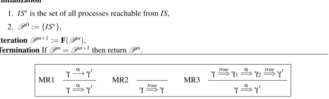
Algorithm 1 Partition-Refinement(IS) Initialization
1. IS?is the set of all processes reachable from IS, 2. P0:= {IS?},
IterationPn+1:= F(Pn),
Termination IfPn=Pn+1then returnPn.
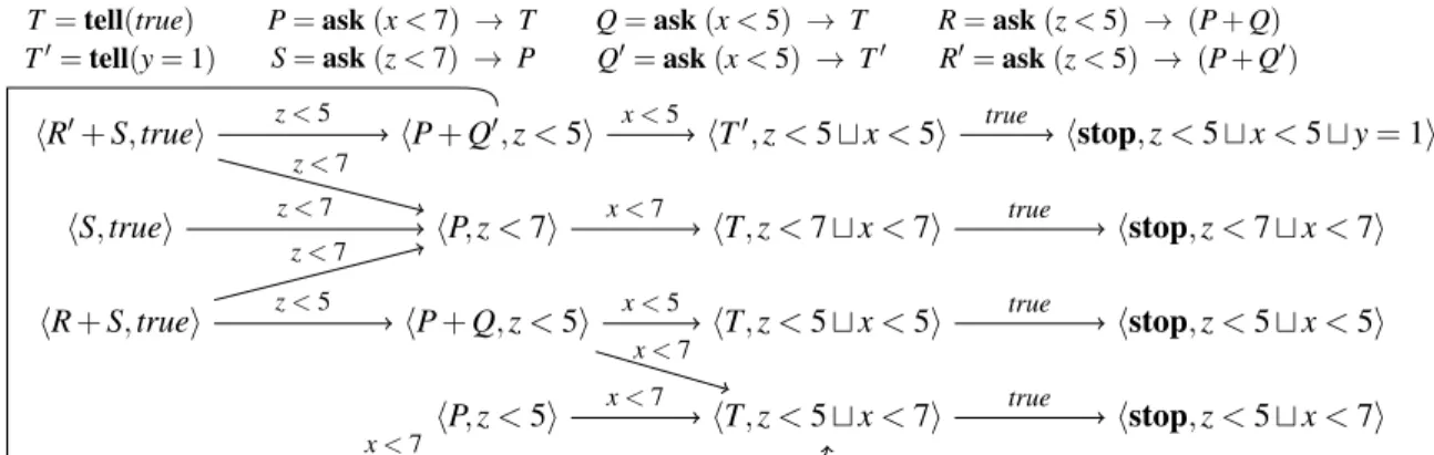
MR1 γ α −→ γ0 γ=⇒ γα 0 MR2 γ=⇒ γtrue MR3 γ true =⇒ γ1 α =⇒ γ2 true =⇒ γ0 γ=⇒ γα 0
Table 1: Milner’s Saturation Method
Standard reduction from weak to strong bisimilarity. As pointed out in the literature (Chapter 3 from [24]), in order to compute weak bisimilarity, we can use the above mentioned partition refinement. The idea is to start from the graph generated via the operational semantics and then saturate it using the rules described in Tab. 1 to produce a new labeled transition relation =⇒. Recall that −→∗ is the reflexive and transitive closure of the transition relation −→. Now the problem whether two states are weakly bisimilar can be reduced to checking whether they are strongly bisimilar wrt =⇒ using partition refinement. As we will show later on, this approach does not work in a formalism like concurrent constraint programming. We shall see that the problem involves the ccp transition labels which, being constraints, can be arbitrary combined using the lub operation t to form a new one. Such a situation does not arise in CCS-like labelled transitions.
Notation 1. When the label of a transition is true we will omit it. Namely, henceforth we will use γ −→ γ0 and γ =⇒ γ0to denote γ −→ γtrue 0and γ=⇒ γtrue 0.
2.1 CCP
We shall now recall ccp and the adaptation of the partition refinement algorithm to compute bisimilarity in ccp [3].
Constraint Systems. The ccp model is parametric in a constraint system (cs) specifying the structure and interdependencies of the information that processes can ask or and add to a central shared store. This information is represented as assertions traditionally referred to as constraints. Following [5, 18] we regard a cs as a complete algebraic lattice in which the ordering v is the reverse of an entailment relation: c v d means d entails c, i.e., d contains “more information” than c. The top element false represents inconsistency, the bottom element true is the empty constraint, and the least upper bound (lub) t is the join of information.
Definition 1 (cs). A constraint system (cs) C = (Con, Con0, v, t, true, false) is a complete algebraic lattice where Con, the set of constraints, is a partially ordered set wrt v, Con0is the subset of compact elements of Con,t is the lub operation defined on all subsets, and true, false are the least and greatest elements of Con, respectively.
R1htell(c), di −→ hstop, d t ci R2 cv d hask (c) → P, di −→ hP, di R3 hP, di −→ hP 0, d0i hP k Q, di −→ hP0k Q, d0i R4 hP, di −→ hP0, d0i hP + Q, di −→ hP0, d0i
Table 2: Reduction semantics for ccp (the symmetric rules for R3 and R4 are omitted).
Remark 1. We shall assume that the constraint system is well-founded and, for practical reasons, that its orderingv is decidable.
We now define the constraint system we use in our examples.
Example 1. Let Var be a set of variables and ω be the set of natural numbers. A variable assignment is a function µ : Var −→ ω. We useA to denote the set of all assignments, P(A ) to denote the powerset ofA , /0 the empty set and ∩ the intersection of sets. Let us define the following constraint system: The set of constraints isP(A ). We define c v d iff c ⊇ d. The constraint false is /0, while true is A . Given two constraints c and d, ct d is the intersection c ∩ d. We will often use a formula like x < n to denote the corresponding constraint, i.e., the set of all assignments that map x to a number smaller than n.
Processes We now recall the basic ccp process constructions. For the sake of space and simplicity we dispense with the recursion operator, which is defined in the standard way as in CCS or other process algebras, and the local/hiding operator (see [2] for further details).
Syntax. Let us presuppose a constraint system C = (Con, Con0, v, t, true, false). The ccp processes are given by the following syntax:
P, Q ::= stop | tell(c) | ask(c) → P | P k Q | P + Q
where c ∈ Con0. Intuitively, stop represents termination, tell(c) adds the constraint (or partial informa-tion) c to the store. The addition is performed regardless the generation of inconsistent information. The process ask(c) → P may execute P if c is entailed from the information in the store. The processes P k Q and P + Q stand, respectively, for the parallel execution and non-deterministic choice of P and Q.
Reduction Semantics. The operational semantics is given by transitions between configurations. A configuration is a pair hP, di representing a state of a system; d is a constraint representing the global store, and P is a process, i.e., a term of the syntax. We use Conf with typical elements γ, γ0, . . . to denote the set of configurations. The operational model of ccp is given by the transition relation −→⊆ Conf× Conf defined in Tab. 2. The rules in Tab. 2 are easily seen to realize the above intuitions.
Barbed Semantics. The authors in [2] introduced a barbed semantics for ccp. Barbed equivalences have been introduced in [21] for CCS, and have become the standard behavioural equivalences for for-malisms equipped with unlabeled reduction semantics. Intuitively, barbs are basic observations (predi-cates) on the states of a system. In the case of ccp, barbs are taken from the underlying set Con0of the constraint system. A configuration γ = hP, di is said to satisfy the barb c (γ ↓c) iff c v d. Similarly, γ satisfies a weak barb c (γ ⇓c) iff there exist γ0s.t. γ −→∗γ0↓c.
In this context, the equivalence proposed is the saturated bisimilarity [7, 6]. Intuitively, in order for two states to be saturated bisimilar, then (i) they should expose the same barbs, (ii) whenever one of them moves then the other should reply and arrive at an equivalent state (i.e. follow the bisimulation game), (iii) they should be equivalent under all the possible contexts of the language. In the case of ccp, it is enough to require that bisimulations are upward closed as in condition (iii) below.
LR1htell(c), di−→ hstop, d tcitrue LR2 α ∈ min{a ∈ Con0| c v d t a } hask (c) → P, di α −→ hP, d t αi LR3 hP, di α −→ hP0, d0i hP k Q, di−→ hPα 0k Q, d0i LR4 hP, di−→ hPα 0, d0i hP + Q, di−→ hPα 0, d0i
Table 3: Labeled semantics for ccp (the symmetric rules for LR3 and LR4 are omitted).
Definition 2 (Saturated Barbed Bisimilarity). A saturated barbed bisimulation is a symmetric relation R on configurations s.t. whenever (γ1, γ2) ∈R with γ1= hP, ci and γ2= hQ, di implies that: (i) if γ1↓e then γ2↓e, (ii) if γ1−→ γ10 then there exists γ20 s.t. γ2−→ γ20 and(γ10, γ20) ∈R, (iii) for every a ∈ Con0, (hP, c t ai, hQ, d t ai) ∈R. We say that γ1and γ2are saturated barbed bisimilar (γ1∼˙sbγ2) if there exists a saturated barbed bisimulationR s.t. (γ1, γ2) ∈R.
We use the term “saturated” to be consistent with the original idea in [7, 6]. However, “saturated” in this context has nothing to do with the Milner’s “saturation” for weak bisimilarity. In the following, we will continue to use “saturated” and “saturation” to denote these two different concepts.
Example 2. Take T = tell(true), P = ask (x < 7) → T and Q = ask (x < 5) → T . You can see thathP,truei 6 ˙∼sbhQ,truei, since hP, x < 7i −→, while hQ, x < 7i 6−→. Consider now the configuration hP + Q,truei and observe that hP + Q,truei ˙∼sbhP,truei. Indeed, for all constraints e, s.t. x < 7 v e, both the configurations evolve intohT, ei, while for all e s.t. x < 7 6v e, both configurations cannot proceed. Since x< 7 v x < 5, the behaviour of Q is somehow absorbed by the behaviour of P.
As we mentioned before, we are interested in deciding the weak version of the notion above. Then, weak saturated barbed bisimilarity( ˙≈sb) is obtained from Def. 2 by replacing the strong barbs in condi-tion (i) for its weak version (⇓) and the transicondi-tions in condicondi-tion (ii) for the reflexive and transitive closure of the transition relation (−→∗).
Labeled Semantics. As explained in [2], in a transition of the form hP, di−→ hPα 0, d0i the label α represents a minimal information (from the environment) that needs to be added to the store d to evolve from hP, di into hP0, d0i, i.e., hP, d t αi −→ hP0, d0i. The labeled transition relation −→ ⊆ Conf × Con0× Conf is defined by the rules in Tab. 3. The rule LR2, for example, says that hask (c) → P, di can evolve to hP, d t αi if the environment provides a minimal constraint α that added to the store d entails c, i.e., α ∈ min{a ∈ Con0| c v d t a}. Note that assuming that (Con, v) is well-founded (Remark 1) is necessary to guarantee that α exists whenever {a ∈ Con0| c v d t a } is not empty. The other rules are easily seen to realize the above intuition. Fig. 1 illustrates the LTSs of our running example.
The labeled semantics is sound and complete wrt the unlabeled one. Soundness states that hP, di−→α hP0, d0i corresponds to our intuition that if α is added to d, P can reach hP0, d0i. Completeness states that if we add a to (the store in) hP, di and reduce to hP0, d0i, it exists a minimal information α v a such that hP, di−→ hPα 0, d00i with d00v d0.
The following lemma is an extension of the one in [2] which considers nondeterministic ccp. Lemma 1 (Correctness of −→). (Soundness) If hP, ci−→ hPα 0, c0i then hP, c t αi −→ hP0, c0i. (Com-pleteness) IfhP, c t ai −→ hP0, c0i then there exists α and b s.t. hP, ci−→ hPα 0, c00i where α t b = a and c00t b = c0.
The above lemma is central for deciding bisimilarity in ccp. In fact, we will show later that for the weak (saturated) semantics the completeness direction does not hold. From this we will show that the standard reduction from weak to strong does not work.
T= tell(true) T0= tell(y = 1) P= ask (x < 7) → T S= ask (z < 7) → P Q= ask (x < 5) → T Q0= ask (x < 5) → T0 R= ask (z < 5) → (P + Q) R0= ask (z < 5) → (P + Q0) hR + S, truei hS, truei hR0+ S, truei hP + Q0, z < 5i hP, z < 7i hP + Q, z < 5i hP, z < 5i hT0, z < 5 t x < 5i hT, z < 7 t x < 7i hT, z < 5 t x < 5i hT, z < 5 t x < 7i hstop, z < 5 t x < 5 t y = 1i hstop, z < 7 t x < 7i hstop, z < 5 t x < 5i hstop, z < 5 t x < 7i x< 7 z< 5 z< 7 z< 7 z< 5 z< 7 x< 5 x< 7 x< 5 x< 7 x< 7 true true true true
Figure 1: The LTS of the running example (IS = {hR0+ S, truei, hS, truei, hR + S, truei}).
2.1.1 Equivalences: Saturated Barbed, Irredundant and Symbolic Bisimilarity
In this section we recall how to check ˙∼sbwith a modified version of partition refinement introduced in [3]. Henceforth, we shall refer to this version as ccp partition refinement (ccp-PR).
The main problem with checking ˙∼sb is the quantification over all contexts. This problem is ad-dressed in [3] following the abstract approach in [8]. More precisely, we use an equivalent notion, namely irredundant bisimilarity ˙∼I, which can be verified with ccp-PR. As its name suggests, ˙∼I only takes into account those transitions deemed irredundant.1 However, technically speaking, going from
˙
∼sb to ˙∼I requires one intermediate notion, so-called symbolic bisimilarity. These three notions are shown to be equivalent, i.e., ˙∼sb= ˙∼sym= ˙∼I. In the following we recall all of them.
Let us first give some auxiliary definitions. The first concept is that of derivation. Consider the following transitions (taken from Fig. 1):
(a) hP + Q, z < 5i−→ hT, z < 5 t x < 7ix<7 (b) hP + Q, z < 5i−→ hT, z < 5 t x < 5ix<5
Transition (a) means that for all constraints e s.t. x < 7 is entailed by e (formally x < 7 v e), the transition (c) hP + Q, z < 5 t ei −→ hT, z < 5 t ei can be performed, while transition (b) means that the reduction (c) is possible for all e s.t. x < 5 v e. Since x < 7 v x < 5, transition (b) is “redundant”, in the sense that its meaning is “logically derived” by transition (a). The following notion captures the above intuition: Definition 3 (Derivation `D). We say that the transition t = hP, ci
α
−→ hP0, c0i derives t0 = hP, ci β −→ hP0, c00i (written t `Dt0) iff there exists e s.t. α t e = β and c0t e = c00.
One can verify in the above example that (a) `D (b), and notice that both transitions arrive at the same process P0, the difference lies in the label and the store. Now imagine the situation where the initial configuration is able to perform another transition with β (as in t0), let us also assume that such transition arrives at a configuration which is equivalent to the result of t0. Therefore, it is natural to think that, since t dominates t0, such new transition should also be dominated by t. Let us explain with an example, consider the two following transitions:
(e) hR + S, truei−→ hP, z < 7iz<7 (f) hR + S, truei−→ hP + Q, z < 5iz<5
Note that transition (f) cannot be derived by other transitions, since (e) 6`D(f). Indeed, P is syntactically different from P + Q, even if they have the same behaviour when inserted in the store z < 5, i.e., hP, z < 5i ˙∼sbhP + Q, z < 5i (since ˙∼sbis upward closed). Transition (f) is also “redundant”, since its behaviour “does not add anything” to the behavior of (e). The following definition encompasses this situation: Definition 4 (Derivation w.r.tR, `R). We say that the transition t = γ−→ γα 1derives t0= γ
β
−→ γ2w.r.t. toR (written t `Rt0) iff there exists γ20 s.t. t`Dγ
β
−→ γ20 and γ20Rγ2.
Then, when R represents some sort of equivalence, this notion will capture the situation above mentioned. Notice that `Dis `R withR being the identity relation (id). Now we introduce the concept of domination, which consists in strengthening the notion of derivation by requiring labels to be different. Definition 5 (Domination D). We say that the transition t = hP, ci
α
−→ hP0, c0i dominates t0= hP, ci−→β hP0, c00i (written t
Dt0) iff t`Dt0and α 6= β .
Similarly, as we did for derivation, we can define domination depending on a relation. Again, Dis just R whenR is the identity relation (id).
Definition 6 (Redundancy and Domination w.r.tR, R). We say that the transition t = hP, ci−→ hPα 0, c0i dominates t0= hP, ci−→ hQ, di w.r.t. toβ R (written t Rt0) iff there exists c00s.t. t DhP, ci
β
−→ hP0, c00i andhP, c00iRhQ,di. Also, a transition is said to be redundant when it is dominated by another, otherwise it is said to be irredundant.
We are now able to introduce symbolic bisimilarity. Intuitively, two configurations γ1 and γ2 are symbolic bisimilar iff (i) they have the same barbs and (ii) whenever there is a transition from γ1 to γ10 using α, then we require that γ2 must reply with a similar transition γ2−→ γα 20 (where γ10 and γ20 are now equivalent) or some other transition that derives it. In other words, the move from the defender does not need to use exactly the same label, but a transition that is “stronger” (in terms of derivation `D) could also do the job. Formally we have the definition below.
Definition 7 (Symbolic Bisimilarity). A symbolic bisimulation is a symmetric relation R on config-urations s.t. whenever (γ1, γ2) ∈R with γ1= hP, ci and γ2 = hQ, di implies that: (i) if γ1 ↓e then γ2↓e, (ii) if hP, ci
α
−→ hP0, c0i then there exists a transition t = hQ, di β
−→ hQ0, d00i and a store d0 s.t. t`DhQ, di−→ hQα 0, d0i and hP0, c0iRhQ0, d0i We say that γ1and γ2are symbolic bisimilar (γ1∼˙symγ2) if there exists a symbolic bisimulationR s.t. (γ1, γ2) ∈R.
Example 3. To illustrate the notion of ˙∼symwe take hP + Q,truei and hP,truei from Ex. 2. We provide a symbolic bisimulationR = {(hP + Q,truei,hP,truei)} ∪ id to prove hP + Q,truei ˙∼symhP,truei. We take the pair (hP + Q,truei, hP,truei). The first condition in Def. 7 is trivial. For the second one, we take hP + Q, truei−→ hT, x < 5i and one can find transitions t = hP, trueix<5 −→ hT, x < 7i and tx<7 0= hP, truei−→x<5 hT, x < 5i s.t. t `Dt0and hT, x < 5iRhT,x < 5i. The restant pairs are trivially verified.
And finally, the irredundant version, which follows the standard bisimulation game where labels need to be matched, however only those transitions so-called irredundant must be considered.
Definition 8 (Irredundant Bisimilarity). An irredundant bisimulation is a symmetric relationR on con-figurations s.t. whenever (γ1, γ2) ∈R implies that: (i) if γ1↓e then γ2↓e, (ii) if γ1 −→ γα 10 and it is irredundant inR then there exists γ20 s.t. γ2−→ γα 20 and(γ10, γ20) ∈R. We say that γ1and γ2 are irredun-dant bisimilar (γ1∼˙Iγ2) if there exists an irredundant bisimulationR s.t. (γ1, γ2) ∈R.
Example 4. We can verify that the relation R in Ex. 3 is an irredundant bisimulation to show that hP + Q,truei ˙∼IhP,truei. We take the pair (hP + Q, truei, hP, truei). The first item in Def. 8 is obvious. Then take hP + Q, truei−→ hT, x < 7i, which is irredundant according to Def. 6, then there exists ax<7 hT, x < 7i s.t. hP, truei−→ hT, x < 7i and (hT, x < 7i, hT, x < 7i) ∈x<7 R. The other pairs are trivially proven. Notice that hP+Q, truei−→ hT, x < 7i x<7 RhP+Q, truei−→ hT, x < 5i hence hP+Q, trueix<5 −→ hT, x < 5ix<5 is redundant, thus it does not need to be matched by hP, truei.
As we said at the beginning, the above-defined equivalences coincide with ˙∼sb. The proof, given in [3], strongly relies on Lemma 1.
Theorem 1. hP, ci ˙∼IhQ, di iff hP, ci ˙∼symhQ, di iff hP, ci ˙∼sbhQ, di 2.1.2 Partition Refinement for CCP
In [3] the authors introduced an algorithm for checking ˙∼sb, by modifying the partition refinement algo-rithm so that to exploit ˙∼I. First, since configurations satisfying different barbs are surely different, it can be safely started with a partition that equates all and only those states satisfying the same barbs. Note that two configurations satisfy the same barbs iff they have the same store. Thus, we take as initial partition P0= {IS?
d1} . . . {IS
?
dn}, where IS
?
di is the subset of the configurations of IS
? with store d
i.2 Secondly, instead of using the function F of Alg. 1, the partitions are refined by employing the function IR defined as follows: for all partitionsP, γ1IR(P)γ2iff
• if γ1−→ γα 10 is irredundant inP, then there exists γ20 s.t. γ2−→ γα 20 and γ10Pγ20. These two steps are the main idea behind the computation of ˙∼I(Alg. 2).
Algorithm 2 CCP-Partition-Refinement(IS) Initialization 1. Compute IS?new 2. P0:= {IS? d1} . . . {IS ? dn}, IterationPn+1:= IR(Pn)
Termination IfPn=Pn+1then returnPn.
2.2 Incompleteness of Milner’s saturation method in ccp
As mentioned at the beginning of this section, the standard approach for deciding weak equivalences is to add some transitions to the original processes, so-called saturation, and then check for the strong equivalence. In calculi like CCS, such saturation consists in forgetting about the internal actions that make part of a sequence containing one observable action (Tab. 1). However, for ccp this method does not work. The problem is that the transition relation proposed by Milner is not complete for ccp, hence the relation among the saturated, symbolic and irredundant equivalences is broken. In the next section we will provide a stronger saturation, which is complete, and allow us to use the ccp-PR to compute ˙≈sb. Let us show why Milner’s approach does not work. First, we need to introduce formally the concept of completeness for a given transition relation.
2In fact, in order to check redundancy, some new states should be added to the initial ones (hence the subscript new in
IS?new). The details of the computation are omitted given that they are not relevant for this paper, however the interested reader
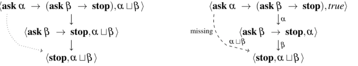
hask α → (ask β → stop), α t β i hask β → stop, α t β i
hstop, α t β i
hask α → (ask β → stop), truei hask β → stop, αi
hstop, α t β i α
β missing
α t β
Figure 2: Counterexample for completeness using Milner’s saturation method (cycles from MR2 omit-ted). Both graphs are obtained by applying the rules in Tab. 1.
Definition 9. We say that a transition relation ⊆ Conf × Con0× Conf is complete iff whenever hP, c t ai hP0, c0i then there exist α, b ∈ Con0s.t.hP, ci hPα 0, c00i where α t b = a and c00t b = c0.
Notice that −→ (i.e the reduction semantics, see Table 2) is complete, and it corresponds to the second item of Lemma 1. Now Milner’s method defines a new transition relation =⇒ using the rules in Tab. 1, but it turns out not to be complete.
Proposition 1. The relation =⇒ defined in Table 1 is not complete.
Proof. We will show a counter-example where the completeness for =⇒ does not hold. Let P = ask α → (ask β → stop) and d = α t β . Now consider the transition hP, di =⇒ hstop, di and let us apply the completeness lemma, we can take c = true and a = α t β , therefore by completeness there must exist band λ s.t. hP, truei=⇒ hstop, cλ 00i where λ t b = α t β and c00t b = d. However, notice that the only transition possible is hP, truei=⇒ hask β → stop, αi, hence completeness does not hold since there isα no transition from hP, truei to hstop, c00i for some c00. Fig. 2 illustrates the problem.
We can now use this fact to see why the method does not work for computing ˙≈sb using ccp-PR. First, let us redefine some concepts using the new transition relation =⇒. Because of condition (i) in
˙
≈sb, we need a new definition of barbs, namely weak barbs w.r.t. =⇒.
Definition 10. We say γ has a weak barb e w.r.t. =⇒ (written γ e) iff γ =⇒∗γ0↓e.
Using this notion, we introduce Symbolic and Irredundant bisimilarity w.r.t. =⇒, denoted by ˙∼=⇒ sym and ˙∼=⇒
I respectively. They are defined as in Def. 7 and 8 where in condition (i) weak barbs (⇓) are replaced with and in condition (ii) the transition relation is now =⇒.
One would expect that since ˙∼sb= ˙∼sym= ˙∼Ithen the natural consequence will be that ˙≈sb= ˙∼=⇒sym= ˙
∼=⇒
I , given that these new notions are supposed to be the weak versions of the former ones when using the saturation method. However, completeness is necessary for proving ˙∼sb= ˙∼sym= ˙∼I, and from Proposition 1 we know that =⇒ is not complete hence we might expect ˙≈sb6= ˙∼=⇒sym6= ˙∼=⇒I . In fact, the following counter-example shows these inequalities.
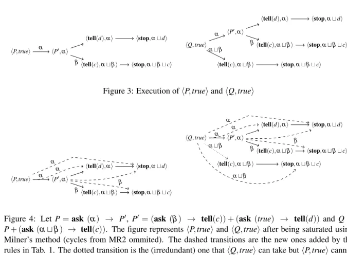
Example 5. Let P, P0 and Q as in Fig. 4. The figure shows hP, truei and hQ, truei after we saturate them using Milner’s method. First, notice thathP, truei ˙≈sbhQ, truei, since there exists a saturated weak barbed bisimulation R = {(hP,truei,hQ,truei)} ∪ id. However, hP, truei 6 ˙∼=⇒
I hQ, truei. To prove that, we need to pick an irredundant transition from hP, truei or hQ, truei (after saturation) s.t. the other cannot match. Thus, take hQ, truei−→ htell(c), α t β i which is irredundant and given that hP, trueiα tβ does not have a transition with α t β then we know that there is no irredundant bisimulation containing (hP, truei, hQ, truei) therefore hP, truei 6 ˙∼=⇒
I hQ, truei. Using the same reasoning we can also show that ˙
hP, truei hP0, αi htell(d), αi htell(c), α t β i hstop, α t β t ci hstop, α t di α β hQ, truei hP0, αi htell(d), αi htell(c), α t β i hstop, α t β t ci hstop, α t di htell(c), α t β i hstop, α t β t ci α β α t β
Figure 3: Execution of hP, truei and hQ, truei
hP, truei hP0, αi htell(d), αi htell(c), α t β i hstop, α t β t ci hstop, α t di α β α α β hQ, truei hP0, αi htell(d), αi htell(c), α t β i hstop, α t β t ci hstop, α t di htell(c), α t β i hstop, α t β t ci α β α t β α t β α α β
Figure 4: Let P = ask (α) → P0, P0 = (ask (β ) → tell(c)) + (ask (true) → tell(d)) and Q = P+ (ask (α t β ) → tell(c)). The figure represents hP, truei and hQ, truei after being saturated using Milner’s method (cycles from MR2 ommited). The dashed transitions are the new ones added by the rules in Tab. 1. The dotted transition is the (irredundant) one that hQ, truei can take but hP, truei cannot match, therefore showing that hP, truei 6 ˙∼=⇒
I hQ, truei
3
Reducing weak bisimilarity to Strong in CCP
In this section we shall provide a method for deciding weak bisimilarity in ccp. As shown in Sec. 2.2, the usual method for deciding weak bisimilarity (introduced in Sec. 2) does not work for ccp. We shall proceed by redefining =⇒ in such a way that it is sound and complete for ccp. Then we prove that, w.r.t. =⇒, symbolic and irredundant bisimilarity coincide with ˙≈sb, i.e. ˙≈sb= ˙∼=⇒sym= ˙∼=⇒I . We therefore conclude that the partition refinement algorithm in [3] can be used to verify ˙≈sbw.r.t. =⇒.
3.1 Defining a new saturation method for CCP
If we analyze the counter-example to completeness (see Fig. 2), one can see that the problem arises because of the nature of the labels in ccp, namely using this method hask α → (ask β → stop), truei does not have a transition with α t β to hstop, α t β i, hence that fact can be exploited to break the relation among the weak equivalences. Following this reasoning, instead of only forgetting about the silent actions we also take into account that labels in ccp can be added together. Thus we have a new rule that creates a new transition for each two consecutive ones, whose label is the lub of the labels in them. This method can also be thought as the reflexive and transitive closure of the labeled transition relation (−→). This transition relation turns out to be sound and complete and it can be used to decide ˙α ≈sb.
R-Tau γ =⇒ γ R-Label γ α −→ γ0 γ=⇒ γα 0 R-Add γ α =⇒ γ0=⇒ γβ 00 γ=⇒ γα tβ 00
Table 4: New Labelled Transition System.
3.1.1 A new saturation method
Formally, our new transition relation =⇒ is defined by the rules in Tab. 4. For simplicity, we are using the same arrow =⇒ to denote this transition relation. Consequently the definitions of weak barbs, symbolic and irredundant bisimilarity are now interpreted w.r.t. =⇒ ( , ˙∼
=⇒
sym and ˙∼=⇒I respectively). First, coincides with ⇓, since a transition in =⇒ corresponds to a sequence of reductions. Lemma 2. γ −→∗γ0iff γ =⇒ γ0.
Using this lemma, it is straightforward to see that the notions of weak barbs coincide. Proposition 2. γ ⇓eiff γ e.
An important property is that the new labeled transition system (=⇒) is finitely branching. Under the assumption that the transition relation −→ is finitely branching and that the amount of states in the transition system is finite, this way, we can use the fact that labels in ccp are idempotent to prove that =⇒ is finitely branching. Formally:
Proposition 3. If for any γ we have |{(γ0, α)|∃α.γ −→ γα 0}| < ∞ and |{γ0|∃α1, . . . , αn.γ α1
−→ . . . αn
−→ γ0}| < ∞, then |{(γ0, α)|∃α.γ=⇒ γα 0}| < ∞.
3.1.2 Soundness and Completeness
As mentioned before, soundness and completeness of the relation are the core properties when proving ˙
∼sb= ˙∼sym= ˙∼I. We now proceed to show that our method enjoys of these properties and they will allow us to prove the correspondence among the equivalences for the weak case.
Lemma 3 (Soundness of =⇒). If hP, ci=⇒ hPα 0, c0i then hP, c t αi =⇒ hP0, c0i. Proof. We proceed by induction on the depth of the inference of hP, ci=⇒ hPα 0, c0i.
• Using R-Tau we have hP, ci =⇒ hP, ci and the result follows directly given that α = true.
• Using R-Label we have hP, ci=⇒ hPα 0, c0i then hP, ci−→ hPα 0, c0i. By Lemma 1 (soundness of −→) we get hP, c t αi −→ hP0, c0i and finally by rule R-Label hP, c t αi =⇒ hP0, c0i.
• Using R-Add then we have hP, ci=⇒ hPβ tλ 0, c0i then hP, ci=⇒ hPβ 00, c00i=⇒ hPλ 0, c0i where β t λ = α. By induction hypothesis, hP, ctβ i =⇒ hP00, c00i (1) and hP00, c00tλ i =⇒ hP0, c0i (2). By monotonic-ity on (1), hP, c t β t λ i =⇒ hP00, c00t λ i and by rule R-Add on this transition and (2) then, given that β t λ = α, we obtain hP, c t αi =⇒ hP0, c0i.
Lemma 4 (Completeness of =⇒). If hP, c t ai =⇒ hP0, c0i then there exist α and b s.t. hP, ci=⇒ hPα 0, c00i where α t b = a and c00t b = c0.
Proof. Assuming that hP, c t ai =⇒ hP0, c0i then, from Lemma 2, we can say that hP, c t ai −→∗hP0, c0i which can be written as hP, c t ai −→ . . . −→ hPi, cii −→ hP0, c0i, we will proceed by induction on i. (Base Case) Assuming i = 0 then hP, c t ai −→ hP0, c0i and the result follows directly from Lemma 1
(Com-pleteness of −→) and R-Label .
(Induction) Let us assume that hP, c t ai −→i hPi, cii −→ hP0, c0i then by induction hypothesis there exist β and b0s.t. hP, ci=⇒ hPβ i, c0ii (1) where β t b0= a and c0it b0= ci. Now by completeness on the last transition hPi,
c0itb0
z}|{
ci i −→ hP0, c0i, there exists λ and b00s.t. hPi, c0ii λ
−→ hP0, c00i where λ t b00= b0 and c00t b00= c0, thus by rule R-Label we have hPi, c0ii
λ
=⇒ hP0, c00i (2). We can now proceed to apply rule R-Add on (1) and (2) to obtain the transition hP, ci=⇒ hPα 0, c00i where α = β t λ and finally take b = b00, therefore the conditions hold α t b = β t λ t b00= a and c00t b = c00t b00= c0.
3.2 Weak saturated bisimilarity coincides with the strong symbolic and irredundant bisimilarity
We show our main result, a method for deciding ˙≈sb. Recall that ˙≈sbis the standard weak bisimilarity for ccp [2], and it is defined in terms of −→, therefore it does not depend on =⇒. Roughly, we start from the fact that ccp-PR is able to check whether two configurations are irredundant bisimilar ˙∼I. Such configurations evolve according to a transition relation (−→), then we provide a new way for them to evolve (=⇒) and we use the same algorithm to compute now ˙∼=⇒
I . Here we prove that ˙≈sb= ˙∼=⇒sym= ˙
∼=⇒
I hence we give a reduction from ˙≈sbto ˙∼=⇒I which has an effective decision procedure.
Given that the transition relation −→ (see Lemma 1) is sound and complete, the correspondence between the symbolic and irredundant bisimilarity follows from [3].
Corollary 1. γ ˙∼=⇒
symγ0iff γ ˙∼=⇒I γ0
Finally, in the next two lemmata, we prove that ˙≈sb= ˙∼=⇒sym. Lemma 5. If γ ˙≈sbγ0then γ ˙∼=⇒symγ0
Proof. We need to prove thatR = {(hP,ci,hQ,di) | hP,ci ˙≈sbhQ, di} is a symbolic bisimulation over =⇒. The first condition (i) of the bisimulation follows directly from Proposition 2. As for (ii), let us assume that hP, ci=⇒ hPα 0, c0i then by soundness of =⇒ we have hP, c t αi =⇒ hP0, c0i, now by Lemma 2 we obtain hP, c t αi −→∗hP0, c0i. Given that hP, ci ˙≈sbhQ, di then from the latter transition we can conclude that hQ, d t αi −→∗hQ0, d0i where hP0, c0i ˙≈
sbhQ0, d0i, hence we can use Lemma 2 again to deduce that hQ, d t αi =⇒ hQ0, d0i. Finally, by completeness of =⇒, there exist β and b s.t. t = hQ, di=⇒ hQβ 0, d00i where β t b = α and d00t b = d0, therefore t `
DhQ, di α
=⇒ hQ0, d0i and hP0, c0iRhQ0, d0i. Lemma 6. If γ ˙∼=⇒
symγ0then γ ˙≈sbγ0
Proof. We need to prove thatR = {(hP,c t ai,hQ,d t ai) | hP,ci ˙∼=⇒symhQ, di} is a weak saturated bisim-ulation. First, condition (i) follows form Proposition 2 and (iii) by definition of R. Let us prove condition (ii), assume hP, c t ai −→∗hP0, c0i then by Lemma 2 hP, c t ai =⇒ hP0, c0i. Now by com-pleteness of =⇒ there exist α and b s.t. hP, ci=⇒ hPα 0, c00i where α t b = a and c00t b = c0. Since hP, ci ˙∼=⇒
symhQ, di then we know there exists a transition t = hQ, di β
=⇒ hQ0, d0i s.t. t `DhQ, di α
and (a)hP0, c00i ˙∼=⇒
symhQ0, d00i, by definition of `Dthere exists b0 s.t. β t b0= α and d0t b0= d00. Using soundness of =⇒ on t we get hQ, d t β i =⇒ hQ0, d0i, thus by Lemma 2 hQ, d t β i −→∗hQ0, d0i and finally by monotonicity hQ, d t a z }| { β t b0 | {z } α tbi −→∗hQ0, d00 z }| { d0t b0tbi (1)
Then, the transition hP, c t ai −→∗hP0, c0i can be rewritten as hP, c t ai −→∗hP0, c00t bi, and using (1), hQ, d t ai −→∗hQ0, d00t bi. It is left to prove that hP0, c00t biRhQ0, d00t bi which follows from (a).
Using Lemma 5 and Lemma 6 we obtain the following theorem. Theorem 2. hP, ci ˙∼=⇒
symhQ, di iff hP, ci ˙≈sbhQ, di
From the above results, we conclude that ˙≈sb= ˙∼=⇒I . Therefore, given that using ccp-PR in combi-nation with =⇒ (and ⇓) we can decide ˙∼=⇒
I , then we can use the same procedure to check whether two configurations are in ˙≈sb.
4
Concluding Remarks
We showed that the transition relation given by Milner’s saturation method is not complete for ccp (in the sense of Definition 9). As consequence we also showed that weak saturated barbed bisimilarity ˙≈sb [2] cannot be computed using the ccp partition refinement algorithm for (strong) bisimilarity ccp wrt to this transition relation. We then presented a new transition relation using another saturation mechanism and showed that it is complete for ccp. We also showed that the ccp partition refinement can be used to compute ˙≈sbusing the new transition relation. To the best of our knowledge, this is the first approach to verifying weak bisimilarity for ccp. As future work, we plan to investigate other calculi where the nature of their transitions systems give rise to similar situations regarding weak and strong bisimilarity, in particular timed ccp (tcc) [25], non-deterministic timed ccp (ntcc) [23], universal temporal ccp (utcc) [22] and Epistemic ccp (eccp) [16].
References
[1] L. Aceto, A. Ingolfsdottir & J. Srba (2011): Advanced Topics in Bisimulation and Coinduction, chapter The Algorithmics of Bisimilarity, pp. 100–172. Cambridge University Press.
[2] Andres Aristizabal, Filippo Bonchi, Catuscia Palamidessi, Luis Pino & Frank D. Valencia (2011): Deriving Labels and Bisimilarity for Concurrent Constraint Programming. In: FOSSACS, LNCS, Springer, pp. 138– 152, doi:10.1007/978-3-642-19805-2 10.
[3] Andres Aristizabal, Filippo Bonchi, Luis Pino & Frank D. Valencia (2012): Partition Refinement for Bisimi-larity in CCP. In: SAC, ACM, pp. 88–93, doi:10.1145/2245276.2245296.
[4] Paolo Baldan, Andrea Bracciali & Roberto Bruni (2007): A semantic framework for open processes. Theor. Comput. Sci. 389(3), pp. 446–483, doi:10.1016/j.tcs.2007.09.004.
[5] Frank S. de Boer, Alessandra Di Pierro & Catuscia Palamidessi (1995): Nondeterminism and Infinite Computations in Constraint Programming. Theor. Comput. Sci. 151(1), pp. 37–78, doi:10.1016/0304-3975(95)00047-Z.
[6] Filippo Bonchi, Fabio Gadducci & Giacoma Valentina Monreale (2009): Reactive Systems, Barbed Seman-tics, and the Mobile Ambients. In: FOSSACS, LNCS, Springer, pp. 272–287, doi:10.1007/978-3-642-00596-1 20.
[7] Filippo Bonchi, Barbara K¨onig & Ugo Montanari (2006): Saturated Semantics for Reactive Systems. In: LICS, IEEE, pp. 69–80, doi:10.1109/LICS.2006.46.
[8] Filippo Bonchi & Ugo Montanari (2009): Minimization Algorithm for Symbolic Bisimilarity. In: ESOP, LNCS, Springer, pp. 267–284.
[9] Roberto Bruni, Fabio Gadducci, Ugo Montanari & Pawel Sobocinski (2005): Deriving Weak Bisimulation Congruences from Reduction Systems. In: CONCUR, LNCS, Springer, pp. 293–307.
[10] Roberto Bruni, Hern´an C. Melgratti & Ugo Montanari (2011): A Connector Algebra for P/T Nets Interac-tions. In: CONCUR, LNCS, Springer, pp. 312–326, doi:10.1007/978-3-642-23217-6 21.
[11] Jean-Claude Fernandez (1989): An Implementation of an Efficient Algorithm for Bisimulation Equivalence. Sci. Comput. Program. 13(1), pp. 219–236, doi:10.1016/0167-6423(90)90071-K.
[12] G.L. Ferrari, S. Gnesi, U. Montanari, M. Pistore & G. Ristori (1998): Verifying Mobile Processes in the HAL Environment. In: CAV, Springer, pp. 511–515.
[13] Fabio Gadducci & Ugo Montanari (2000): The tile model. In: Proof, Language, and Interaction, The MIT Press, pp. 133–166.
[14] O. H. Jensen. (2006): Mobile Processes in Bigraphs. Ph.D. thesis, University of Cambridge.
[15] Paris C. Kanellakis & Scott A. Smolka (1983): CCS Expressions, Finite State Processes, and Three Problems of Equivalence. In: PODC, ACM, pp. 228–240.
[16] Sophia Knight, Catuscia Palamidessi, Prakash Panangaden & Frank D. Valencia (2012): Spatial Information Distribution in Constraint-based Process Calculi (Extended Version). Technical Report, INRIA.
[17] Ivan Lanese, Jorge A. P´erez, Davide Sangiorgi & Alan Schmitt (2011): On the expressiveness and decidabil-ity of higher-order process calculi. Inf. Comput. 209(2), pp. 198–226, doi:10.1016/j.ic.2010.10.001. [18] N. P. Mendler, Prakash Panangaden, Philip J. Scott & R. A. G. Seely (1995): A Logical View of Concurrent
Constraint Programming. Nord. J. Comput. 2(2), pp. 181–220.
[19] Robin Milner (1980): A Calculus of Communicating Systems. Lecture Notes in Computer Science 92, Springer-Verlag New York, Inc., doi:10.1007/3-540-10235-3.
[20] Robin Milner (1999): Communicating and mobile systems: the π-calculus. Cambridge University Press. [21] Robin Milner & Davide Sangiorgi (1992): Barbed Bisimulation. In: ICALP, LNCS, Springer, pp. 685–695. [22] Carlos Olarte & Frank D. Valencia (2008): Universal concurrent constraint programing: symbolic semantics
and applications to security. In: SAC, ACM, pp. 145–150.
[23] Catuscia Palamidessi & Frank D. Valencia (2001): A Temporal Concurrent Constraint Programming Calcu-lus. In: CP, LNCS, Springer, pp. 302–316.
[24] Davide Sangiorgi & Jan Rutten (2012): Advanced Topics in Bisimulation and Coinduction. Cambridge University Press.
[25] Vijay A. Saraswat, Radha Jagadeesan & Vineet Gupta (1994): Foundations of Timed Concurrent Constraint Programming. In: LICS, IEEE, pp. 71–80.
[26] Vijay A. Saraswat & Martin C. Rinard (1990): Concurrent Constraint Programming. In: POPL, ACM Press, pp. 232–245.
[27] Vijay A. Saraswat, Martin C. Rinard & Prakash Panangaden (1991): Semantic Foundations of Concurrent Constraint Programming. In: POPL, ACM Press, pp. 333–352.
[28] Pawel Sobocinski (2010): Representations of Petri Net Interactions. In: CONCUR, LNCS, Springer, pp. 554–568.
[29] Pawel Sobocinski (2012): Relational presheaves as labelled transition systems. In: In proceedings CMCS, To appear in LNCS.
[30] Bj¨orn Victor & Faron Moller (1994): The Mobility Workbench - A Tool for the pi-Calculus. In: CAV, LNCS, Springer, pp. 428–440.