SHORTEST PATH RESOLUTION USING HADOOP

HAL Id: hal-01166678

https://hal.archives-ouvertes.fr/hal-01166678

Submitted on 23 Jun 2015

HAL is a multi-disciplinary open access

archive for the deposit and dissemination of

sci-entific research documents, whether they are

pub-lished or not. The documents may come from

teaching and research institutions in France or

abroad, or from public or private research centers.

L’archive ouverte pluridisciplinaire HAL, est

destinée au dépôt et à la diffusion de documents

scientifiques de niveau recherche, publiés ou non,

émanant des établissements d’enseignement et de

recherche français ou étrangers, des laboratoires

publics ou privés.

Sabeur Aridhi, Vincent Benjamin, Philippe Lacomme, Libo Ren

To cite this version:

Sabeur Aridhi, Vincent Benjamin, Philippe Lacomme, Libo Ren. SHORTEST PATH RESOLUTION

USING HADOOP . MOSIM 2014, 10ème Conférence Francophone de Modélisation, Optimisation et

Simulation, Nov 2014, Nancy, France. �hal-01166678�

SHORTEST PATH RESOLUTIONUSING HADOOP

Sabeur Aridhi, Vincent Benjamin, Philippe Lacomme, Libo Ren

Laboratoire d'Informatique de Modélisation et d‟Optimisation des Systèmes (LIMOS, UMR CNRS 6158),

Campus des Cézeaux, 63177 Aubière Cedex, France {aridhi, benjamin.vincent, placomme, ren}@isima.fr

ABSTRACT: The fast growth of scientific and business data has resulted in the evolution of the cloud computing. The MapReduce

parallel programming model is a new framework favoring design of algorithms for cloud computing. Such framework favors processing problems across huge datasets using a large number of computers. Hadoop is an implementation of MapReduce framework that becomes one of the most interesting approaches for cloud computing. Our contribution consists in investigating how the MapReduce framework can create new trend in design of operational research algorithms and could define a new methodology to adapt algorithms to Hadoop. Our investigations are directed on the shortest path problem on large-scale real-road networks. The proposed algorithm is tested on a graph modeling French road network using the OpenStreetMap data. The computational results push us into considering that Hadoop offers a promising approach for problems where data are so large that numerous memory problems and excessive computational time could arise using a classical resolution scheme.

KEYWORDS: Shortest path, cloud, hadoop, MapReduce.

1 INTRODUCTION

The rapid growth of internet since last decades has led to a huge amount of information which has created a trend in design of modern data center and massive data processing algorithms especially in the cloud. Hadoop is one of the most interesting approaches for cloud computing which is an implementation of MapReduce framework first introduced and currently promoted by Google. In this article, we are interested in evaluating how hadoop framework offers a promising approach for operational research algorithms. Here we consider the shortest path problem (SPP) on large-scale real-road networks. The adaptation of shortest path algorithms (commonly used in resolution of scheduling problems or routing problems) for the clouds, required attention since the applications must be tuned to frameworks which take advantages of the cloud resources (Srirama et al., 2012).

1.1 Shortest path problems

Shortest path problems drawn attention for use in various transportation engineering applications. Without any doubt it could be directly attributed to the recent developments in Intelligent Transportation Systems (ITS), particularly in the field of Route Guidance System (RGS). The current RGS field in both North America and Europe has generated new interest in using heuristic algorithms to find shortest paths in a traffic network for vehicle routing operations. (Guzolek and Koch, 1989) discussed how heuristic search methods could be tuned for vehicle navigation systems. (Kuznetsov, 1993)

debates applications of an A* algorithm, a bi-directional search methods, and a hierarchical search one.

Several researchers have been addressed the definition of efficient search strategies and mechanisms. For example, the multi-objective shortest path problem is addressed by Umair et al. in 2014 (Umair et al., 2014). They introduced an evolutionary algorithm for the MOSP (Multi-Objective Shortest Path). They have also presented a state of the art on the MOSP where publications are gathered into classes depending on the approaches. Some authors including, but not limited to (Tadao, 2014), introduced new advance in complexity improvement in classical shortest path algorithms based on bucket approaches. (Cantone and Faro, 2014) introduced lately a hybrid algorithms for the Single Source Shortest Paths (and all-pairs SP) which is asymptotically fast in some special graph configurations. A recent survey of (Garroppo et al., 2010) focuses on the multi-constrained approximated shortest path algorithms representing by recent publications of (Gubichev et al., 2010) or (Willhalm, 2005).

1.2 Parallel data-processing paradigm with hadoop

Hadoop is an open-source Apache project which provides solutions for storage and large-scale distributed computing. It relies on two components: the first one Hadoop Distributed File System (HDFS) which allows to store large files across multiple computers; the second component is the wide spread MapReduce engine (Dean J. and S. Ghemawat, 2008) which provides a programming model for large-scale distributed computing.

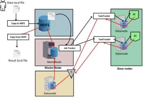
As stressed in the figure 1, a hadoop system consists of a master and several slave nodes. The master should consist a NameNode and a JobTracker to manage respectively data storage and computation jobs scheduling. A slave node could be a DataNode for data

storage or/and a TaskTracker for processing computation jobs. A secondary NameNode can be used to replicate data of the NameNode to provide a high quality of service. HDFS Datanode Datanode Slave nodes NameNode Job Tracker TaskTracker TaskTracker

Data local file

Copy to HDFS

Copy from HDFS

Result local file

Datanode Slave nodes Master Node

Figure 1: Typical component of one hadoop cluster Hadoop uses the MapReduce engine as the parallel

data-processing paradigm. Cohen in 2009 (Cohen, 2009) prove that MapReduce could be successfully applied for specific graph problems, including but not limited to computation of graph components, clustering, rectangles/triangles enumeration. MapReduce has also been used for scientific problems by (Bunch et al., 2009) proving that it could be used to solve problems including the Marsaglia polar method for generating random variables and integer sort. In (Sethia and Karlapalem, 2011), the authors explore the benefits hadoop-based multi-agents simulation framework implementation.

1.3 Hadoop terminology

In hadoop terminology, by „job‟ we mean execution of a Mapper and Reducer across a data set and by „task‟ we

mean an execution of a Mapper or a Reducer on a slice of data. Hadoop distributes the Map invocations across several computers by partitioning the input data automatically into a set of independent splits. Those input splits are processed in parallel as Mapper tasks on slave nodes.

Hadoop invokes a Record Reader method on the input split to read one record per line until the entire input split has been consumed. Each call of the Record Reader leads to another call to the Map function of the Mapper. Reduce invocations are distributed by splitting the key space into pieces using a splitting function. One more thing to mention here is that some problems require a succession of MapReduce steps to accomplish their goals. Partition 1 HDFS Partition 2 Partition n Map () Map by Data ID Map by Data ID Map by Data ID Execute job on node Reduce () Collect Data ID Collect Data ID Collect Data ID Generate the output data

Figure 2: MapReduce Flow As shown in figure 2, a MapReduce task consists in two

following steps: first the Map tasks are scheduled and second the Reduce tasks. It gets periodic updates from

the datanodes about the average time on each datanode. The information on average time permits distribution of tasks favoring the faster datanodes.

Hadoop is a new trend in parallel and distributed computing. Providing a full integration into cloud architectures, hadoop permits to operational researchers to focus on the parallelization of algorithms without consideration of the network infrastructure required to achieve the computation. Hadoop is now proposed in numerous public and private cloud solutions including AWS, Google, IBM and Azure. Hadoop is a very interesting solution since it permits for a reasonable effort to create new parallel implementation of various algorithms.

This paper is organized as follow. In the next section, we present the proposed MapReduce-based method for large-scale shortest path problem. In Section 3, we describe the experimental study using large real-world

road networks. In Section 4, we conclude the work and we highlight some future works.

2 SHORTEST PATH RESOLUTION WITH

HADOOP

2.1 Framework description

In the proposed framework for the shortest path computation, each iteration represents a single MapReduce pass. As stressed by (Srirama et al., 2012), such type of resolution scheme is difficult to benefit efficiently from parallelization, and the proposed framework does not guarantee to solve optimally the shortest path problem but lead to high quality solutions.

Data local file

Partition of the straight line on the graph into nb

subgraphs I : Inital node

J : Final node L : Subgraph size

Ne : maximal number of iterations

HDFS Compute shortest path in the subgraph 1 Compute shortest path in the subgraph nb Wait until node achieved job

Step 1 : Create initial data Step 2 : Computaton of one initial shortest path

Retrieved the shortest path Partition into subgraph HDFS Compute shortest path in the subgraph 1 Compute shortest path in the subgraph nb Wait until node achieved job Retrieved the shortest path

Step 3 : Improvement Step 4 : Retreived solution

Ne iterations

The Shortest path

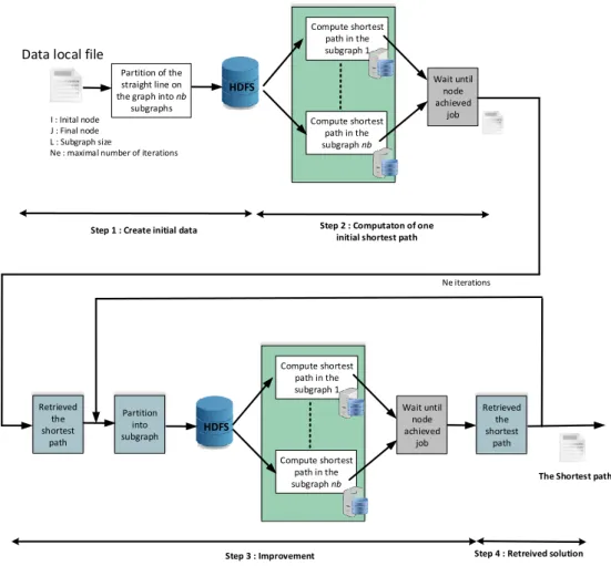
Figure 3: Hadoop based framework for the shortest path

2.2 Proposed algorithm

The hadoop-based shortest path resolution framework consists of 4 steps (see figure 3). The first step consists in uploading data to the hadoop file system. It consists also in specifying parameters like the initial/final positions, the maximal number of iterations and the subgraphs size. The second step aims to calculate one shortest path (Initial Shortest Path) which is iteratively improved in the next step. The initial shortest path computation begins with the creation of subgraphs which leads to jobs parallelization since computation of the

shortest path on each subgraph (noted as local shortest path) is considered as a job in hadoop. This step 2 is fully achieved when all local shortest paths have been uploaded from slave nodes. The initial shortest path is obtained by concatenating all local shortest paths. The step 3 is an iterative improvement. In this step, a subgraph is defined by the middle points of two adjacent local shortest paths. One can note that the number of subgraphs depends the iteration number. It alternates between and where the number of subgraphs in step 2. The process is stopped when the number of iterations is reached. The step 4 consists in

downloading the results from the hadoop file system to a local directory. In the following, we present the

algorithm of our approach (see Algorithm 1).

Algorithm 1. Hadoop shortest path framework

1. Procedure SSP_Hadoop_Framework

2. Input parameters

3. L : subgraph size in km

4. Ix, Iy : Initial latitude and longitude

5. Jx, Jy : Final latitude and longitude

6. Ne : maximal number of iterations

7. begin

8. // Step 1. Create initial data

9. (G,Dx,Dy,Ax,Ay):= Partition_Into_Subgraph(L,Ix,Iy,Jx,Jy);

10. nb := |G|;

11. // Step 2. Computation of the initial shortest path 12. for j:=1 to nbdo

13. << copy G[j] from local to HDFS >>

14. << G[j] will be copied from HDFS to a slave node >> 15. SP”[j] = Start_Node_Job(G[j],Dx[j],Dy[j],Ax[j],Ay[j]); 16. end for

17. << wait until hadoop nodes have achieved work >> 18. SP:= Retrieved_Shortest_Path(SP”);

19.

20. // Step 3. Improvement of the shortest path 21. for i:=2 to Ne do

22. if (i%2=0) Then

23. for j:=1 to|SP| -1 do

24. (Mx[j], My[j]):= the middle of the shortest path SP[j]; 25. (Mx[j+1], My[j+1]):= the middle of the shortest path SP[j+1]; 26. G[j] := Create_Graph(Mx[j], My[j], Mx[j+1], My[j+1]);

27. << copy G[j] from local to HDFS>>

28. << G[j] will be copied from HDFS to a slave node >>

29. SP”[j]:= Start_Node_Job(G[j], Mx[j], My[j], Mx[j+1], My[j+1]); 30. end for

31. << wait until hadoop nodes have achieved work >>

32. SP’:= Retrieved_Shortest_Path(SP”); 33.

34. // Step 4. Load output files from the HDFS to local directory

35. Load SP’ from the HDFS to local directory 36. else

37. for j:=0 to|SP’|do // size of SP’ = nb-1 38. if(j=0)

39. (Mx[j], My[j]):= (Ix, Iy); 40. else

41. (Mx[j], My[j]):= the middle of the shortest path SP’[j];

42. end if

43. if(j = |SP’|)

44. (Mx[j+1], My[j+1]):= (Jx, Jy); 45. else

46. (Mx[j+1], My[j+1]):= the middle of the shortest path SP’[j+1];

47. end if

48. G[j+1]:= Create_Graph(Mx[j], My[j], Mx[j+1], My[j+1]); 49. << copy G[j+1] from local to HDFS>>

50. << G[j+1] will be copied from HDFS to a slave node >>

51. SP”[j+1]:= Start_Node_Job(G[j], Mx[j], My[j], Mx[j+1], My[j+1]); 52. end for

53. << wait until hadoop nodes have achieved work >> 54. SP:= Retrieved_Shortest_Path(SP”);

55.

56. // Step 4. Download data from HDFS

57. Load SP from the HDFS to local directory 58. end if

59. end for

60. return Concat(SP, SP’, Ne);

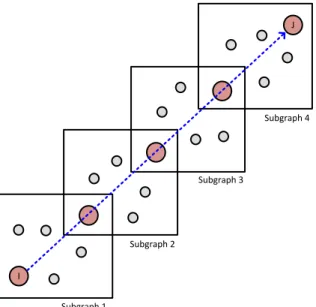
In algorithm 1, lines 8-10 describe the first step. In which, the procedure Partition_Into_Subgraph consists in creation of subgraphs by dividing the “straight line” from an origin to a destination into several subgraphs according the predefined length (the diagonal length of subgraph). The subgraph data is created by extracting road information from the OpenStreetMap data. Figure 4 gives an example of subgraphs creation. It

consists in using the "straight line" from node and to create 4 subgraphs. A subgraph is defined by its origin node and destination node and the origin node of subgraph is the destination node of subgraph.

One can note that the origin position of _{subgraph is}

the destination of subgraph, , where the number of subgraphs.

I J Subgraph 1 Subgraph 2 Subgraph 3 Subgraph 4

Figure 4: First partition and shortest path

Lines 11-18 illustrate the step 2 of algorithm. The procedure Start_Node_Job allows starting the computation of local shortest path on subgraphs using MapReduce engine. The procedure requires a subgraph and the GPS coordinates of the origin and destination positions. In this step, it is possible that an origin or a destination does not correspond to a node of the subgraph. Therefore, a projection step is necessary to compute the nearest node of the subgraph form each GPS position before starting the shortest path computation. A Dijkstra algorithm is adapted here for the shortest path computation. As known, a classical shortest path problem can be solved using Dijkstra's

algorithm in

O



n

log

n



with a priority queue such as a Fibonacci heap (Fredman and Tarjan, 1987) or 2-3 heaps (Takaoka, 1999). The obtained local shortest paths are saved into a vector denoted . One assumes that is the shortest path of the _subgraph.

Lines 21-32 and lines 36-54 describe the improvement step. The call of the procedure Create_Graph consists in creation the subgraphs induced by the middle of the shortest path of the current iteration (lines 24-25). As mentioned before, the subgraph number is different between an odd iteration and an even iteration. As shown in figure 5 (a), we assumes that each square is one subgraph. At one odd iteration , concatenating of the set of local shortest paths gives the initial shortest path from to .

Figure 5 (b) gives a solution at the even iteration . Considering the set of local shortest paths obtained at iteration and , a node (with its coordinates ) is the node corresponds to the middle of in terms of kilometers (the nearest node to the middle of the path). The subgraph creation consists in encompassing the nodes and . In this

example, 3 subgraphs have been created. The obtained set of local shortest paths is denoted . One can note that the concatenations of all local shortest paths do not give the path from to . It is necessary to include the path from the node to and the path from to in order to form a solution to the initial problem. To do so, we have to use the set of local shortest paths obtained at iteration . I P1 J P3 P2 Subgraph 1 Subgraph 2 Subgraph 3 Subgraph 4 SP[1] SP[2] SP[3] SP[4] I P1 J P3 P2 Subgraph 1 Subgraph 2 Subgraph 3 SP’[1] SP’[2] SP’[3] M1 M2 M3 M4

(a) set of LSP at an odd iteration (b) set of LSP at an even iteration

Figure 5: Two adjacent iterations of shortest paths computation Line 34 and line 57 describe the last step which consists

in downloading the results of last of two iterations from the hadoop file system. The shortest path is obtained by

calling the procedure concat which takes 3 parameters including the number of iterations and the solutions of two last iterations.

3 NUMERICAL EXPERIMENTS

All tests were conducted using hadoop 0.23.9 with a cluster of 8 homogenous nodes. Each node is a PC with AMD Opteron processor (2.3 GHz) under Linux (CentOS 64-bit). The number of cores used for experiments is limited to 1. The iteration number of algorithm is set to 2.

3.1 Instances

A graph of French road network has been created using the OpenStreetMap data. The road profile is fixed to pedestrian. A group of 15 instances are created using the same graph. Each instance contains an origin and a destination (see table 1). The subgraph size km is addressed. Note that the graph will not be split into subgraphs when . The used graph can be downloaded from:

http://www.isima.fr/~lacomme/hadoop_mosim/.

Origin Destination

Instance City GPS position City GPS position

1 Clermont-Ferrand 45.779796 3.086371 Montluçon 46.340765 2.606664 2 Paris 48.858955 2.352934 Nice 43.70415 7.266376 3 Paris 48.858955 2.352934 Bordeaux 44.840899 -0.579729 4 Clermont-Ferrand 45.779796 3.086371 Bordeaux 44.840899 -0.579729 5 Lille _{50.63569 3.062081 Toulouse 43.599787 1.431127} 6 Brest 48.389888 -4.484496 Grenoble 45.180585 5.742559 7 Bayonne 43.494433 -1.482217 Brive-la-Gaillarde 45.15989 1.533916 8 Bordeaux 44.840899 -0.579729 Nancy 48.687334 6.179438 9 Grenoble 45.180585 5.742559 Bordeaux 44.840899 -0.579729 10 Reims _{49.258759 4.030817 Montpellier 43.603765 3.877974} 11 Reims 49.258759 4.030817 Dijon 47.322709 5.041509 12 Dijon 47.322709 5.041509 Lyon 45.749438 4.841852 13 Montpellier 43.603765 3.877974 Marseille 43.297323 5.369897 14 Perpignan 42.70133 2.894547 Reims 49.258759 4.030817 15 Rennes _{48.113563 -1.66617 Strasbourg 48.582786 7.751825}

Table 1: Instances data

3.2

Influence of the subgraphs size on the results

quality

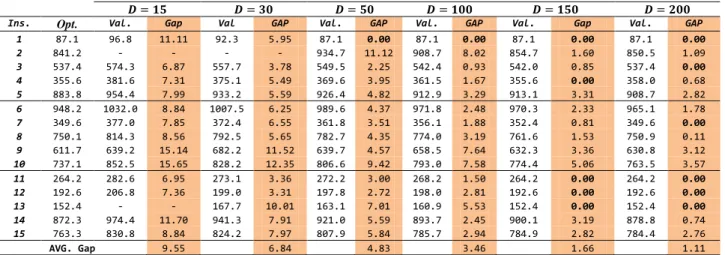
Table 2 contains the computational results for different subgraph sizes from 15 to 200 kilometers. In which, the optimal solutions is obtained using which lead to computation of a shortest path on the whole graph. Column “Ins.” contains the instance; column “Opt.” contains the optimal solution (execution of a Dijkstra algorithm in the whole graph); columns “Val.” reports the obtained value with 2 iterations; and “Gap” is the gap

(%) the best found solution to the optimal value. As shown in in the table 2, the average Gap is improved when we increase subgraph size. More precisely, the average Gap is improved from 9.55% to 1.11%. When km, the optimal solution were obtained for 6 instances out of 15. On the other hand, when km, no feasible solution is found for several instances. Since the nodes distribution could arise several problems of connectivity in small subgraphs.

Ins. Opt. Val. Gap Val GAP Val. GAP Val. GAP Val. Gap Val. GAP

1 87.1 96.8 11.11 92.3 5.95 87.1 0.00 87.1 0.00 87.1 0.00 87.1 0.00 2 841.2 - - - - 934.7 11.12 908.7 8.02 854.7 1.60 850.5 1.09 3 537.4 574.3 6.87 557.7 3.78 549.5 2.25 542.4 0.93 542.0 0.85 537.4 0.00 4 355.6 381.6 7.31 375.1 5.49 369.6 3.95 361.5 1.67 355.6 0.00 358.0 0.68 5 883.8 954.4 7.99 933.2 5.59 926.4 4.82 912.9 3.29 913.1 3.31 908.7 2.82 6 948.2 1032.0 8.84 1007.5 6.25 989.6 4.37 971.8 2.48 970.3 2.33 965.1 1.78 7 349.6 377.0 7.85 372.4 6.55 361.8 3.51 356.1 1.88 352.4 0.81 349.6 0.00 8 750.1 814.3 8.56 792.5 5.65 782.7 4.35 774.0 3.19 761.6 1.53 750.9 0.11 9 611.7 639.2 15.14 682.2 11.52 639.7 4.57 658.5 7.64 632.3 3.36 630.8 3.12 10 737.1 852.5 15.65 828.2 12.35 806.6 9.42 793.0 7.58 774.4 5.06 763.5 3.57 11 264.2 282.6 6.95 273.1 3.36 272.2 3.00 268.2 1.50 264.2 0.00 264.2 0.00 12 192.6 206.8 7.36 199.0 3.31 197.8 2.72 198.0 2.81 192.6 0.00 192.6 0.00 13 152.4 - - 167.7 10.01 163.1 7.01 160.9 5.53 152.4 0.00 152.4 0.00 14 872.3 974.4 11.70 941.3 7.91 921.0 5.59 893.7 2.45 900.1 3.19 878.8 0.74 15 763.3 830.8 8.84 824.2 7.97 807.9 5.84 785.7 2.94 784.9 2.82 784.4 2.76 AVG. Gap 9.55 6.84 4.83 3.46 1.66 1.11

Table 2: Influence of the subgraphs size

3.3 Influences of the number of slave hadoop

nodes

Table 3 reports the computational time with different number of nodes: column “1-sn” for time consumption with one slave node, column “4-sn” for 4 slave nodes resolution time, and column “8-sn” for 8 slave nodes resolution time. One can note that the average computational time varies strongly between the different numbers of slaves and the size of subgraph. For the

instance 2, the computation time decreased from 613 seconds to 76 seconds with km. For several instances, increasing of the salve nodes number does not improve the computational time. For the instance 8with km, the computational time is equal between 4 nodes and 8 nodes. Such analysis pushes us into considering that there exists an optimal configuration on the number of nodes and the subgraph size for resolution of each instance. Ins. 1-sn 4-sn 8-sn 1-sn 4-sn 8-sn 1-sn 4-sn 8-sn 1-sn 4-sn 8-sn 1 84 49 54 55 54 49 51 48 48 60 60 59 2 613 127 76 247 62 55 177 58 58 194 92 92 3 457 106 65 181 61 55 129 59 60 132 78 78 4 281 75 52 122 52 52 97 58 56 80 72 68 5 689 138 76 277 73 58 192 65 63 179 91 88 6 746 149 87 318 75 56 250 74 62 244 92 90 7 274 73 51 119 52 49 88 53 53 81 73 72 8 573 121 69 228 65 51 160 56 54 159 78 81 9 444 102 108 171 55 51 119 55 55 114 75 75 10 530 110 65 203 56 49 142 56 56 152 80 80 11 216 61 49 87 50 51 65 55 51 68 63 64 12 179 54 51 81 52 55 62 58 58 68 67 66 13 137 47 48 66 52 51 60 59 59 59 59 58 14 614 119 76 234 69 53 167 59 53 125 62 64 15 601 122 73 221 61 51 160 63 64 146 72 74 AVG. 429.2 96.9 66.7 174.0 59.3 52.4 127.9 58.4 56.7 124.1 74.3 73.9

Table 3:

Impact of slave nodes number on the computation time

4 CONCLUDING REMARKS

The MapReduce framework is a new approach for operational research algorithms and our contribution stands at the crossroads of optimization research community and map-reduce community. Our contribution consists in proving there is a great interest in defining approaches taking advantages of research coming from information system and parallelization.

As future work, we are interested in adapting the operational research algorithms to such framework, especially for those which could be more easily to take advantages of parallel computing platform as GRASP or Genetic algorithm.

REFERENCES

Bunch C., B. Drawert and M. Norman,. Mapscale: a cloud environment for scientific computing, Technical Report, University of California, Computer Science Department. 2009.

Cantone D. and S. Faro. Fast shortest-paths algorithms in the presence of few destinations of negative-weight arcs. Journal of Discrete Algorithms, Vol. 24, pp. 12-25. 2014.

Cohen J., 2009. Graph twiddling in a MapReduce world, Computing in Science and Engineering. Vol. 11, pp. 29–41. 2009.

Dean J. and S. Ghemawat. Mapreduce: simplified data processing on large clusters. Communications of the ACM, Vol. 51, pp. 107–113. 2008.

Fredman M.L. and R.E. Tarjan. Fibonacci heaps and their uses in improved network optimization algorithms, J. ACM, Vol. 34, pp. 596–615. 1987. Garroppo R.G., S. Giordano and L. Tavanti. 2010. A

survey on multi-constrained optimal path computation: Exact and approximate algorithms. The International Journal of Computer and Telecommunications Networking. Vol. 54(17), pp. 3081-3107. 2010.

Gubichev A., S. Bedathur, S. Seufert and G. Weikum. 2010. Fast and Accurate Estimation of Shortest Paths in Large Graphs. CIKM’10, October 26–30, Toronto, Ontario, Canada. 2010.

Guzolek J, Koch E. Real-time route planning in road network. Proceedings of VINS, September Vol. 11– 13. Toronto, Ontario, Canada, pp. 165–9. 1989. Kuznetsov T. High performance routing for IVHS.IVHS

America 3rd Annual Meeting, Washington, DC, 1993.

Sethia P. and Karlapalem K. A multi-agent simulation framework on small Hadoop cluster. Engineering Applications of ArticifialIntelligence. Vol. 24, pp. 1120-1127. 2011.

Srirama S.N., P. Jakovits and E.Vainikko. Adapting scientific computing problems to clouds using MapReduce. Future Generation Computer Systems. Vol.28, pp. 184–192. 2012.

Tadao T. Sharing information for the all pairs shortest path problem. Theoretical Computer Science, Vol. 520(6), pp. 43-50. 2014.

Takaoka T. Theory of 2–3 heaps. in: COCOON ‟99, in: Lect. Notes Comput. Sci. 1999.

Umair F. Siddiqi, YoichiShiraishi, Mona Dahb and Sadiq M. Sait. A memory efficient stochastic evolution based algorithm for the multi-objective shortest path problem. Applied Soft Computing, Vol. 14, Part C, pp. 653-662. 2014. Willhalm T. Engineering shortest paths and layout

algorithms for large graphs. Karlsruhe Institute of Technology, pp. 1-130. 2005.