HAL Id: hal-00318231
https://hal.archives-ouvertes.fr/hal-00318231
Submitted on 21 Dec 2006
HAL is a multi-disciplinary open access
archive for the deposit and dissemination of
sci-entific research documents, whether they are
pub-lished or not. The documents may come from
teaching and research institutions in France or
abroad, or from public or private research centers.
L’archive ouverte pluridisciplinaire HAL, est
destinée au dépôt et à la diffusion de documents
scientifiques de niveau recherche, publiés ou non,
émanant des établissements d’enseignement et de
recherche français ou étrangers, des laboratoires
publics ou privés.
cloud on the east and west sides of the Scandinavian
mountains and microphysical box model simulations
U. Blum, F. Khosrawi, G. Baumgarten, K. Stebel, R. Müller, K. H. Fricke
To cite this version:
U. Blum, F. Khosrawi, G. Baumgarten, K. Stebel, R. Müller, et al.. Simultaneous lidar observations of
a polar stratospheric cloud on the east and west sides of the Scandinavian mountains and microphysical
box model simulations. Annales Geophysicae, European Geosciences Union, 2006, 24 (12),
pp.3267-3277. �hal-00318231�
www.ann-geophys.net/24/3267/2006/ © European Geosciences Union 2006
Annales
Geophysicae
Simultaneous lidar observations of a polar stratospheric cloud on
the east and west sides of the Scandinavian mountains and
microphysical box model simulations
U. Blum1, F. Khosrawi2, G. Baumgarten3, K. Stebel4, R. M ¨uller5, and K. H. Fricke6
1Forsvarets forskningsinstitutt, 2027 Kjeller, Norway
2Institutionen f¨or till¨ampad milj¨ovetenskap/Meteorologiska institutionen, Stockholms Universitet, 10691 Stockholm, Sweden 3Leibniz-Institut f¨ur Atmosph¨arenphysik e.V., 18225 K¨uhlungsborn, Germany
4Norsk institutt for luftforskning, 9296 Tromsø, Norway
5Institut f¨ur Chemie und Dynamik der Geosph¨are: Stratosph¨are (ICG-I), Forschungszentrum J¨ulich, 52425 J¨ulich, Germany 6Physikalisches Institut der Universit¨at Bonn, 53115 Bonn, Germany
Received: 11 July 2006 – Revised: 6 November 2006 – Accepted: 27 November 2006 – Published: 21 December 2006
Abstract. The importance of polar stratospheric clouds (PSC) for polar ozone depletion is well established. Lidar ex-periments are well suited to observe and classify polar strato-spheric clouds. On 5 January 2005 a PSC was observed si-multaneously on the east and west sides of the Scandinavian mountains by ground-based lidars. This cloud was composed of liquid particles with a mixture of solid particles in the up-per part of the cloud. Multi-colour measurements revealed that the liquid particles had a mode radius of r≈300 nm, a dis-tribution width of σ ≈1.04 and an altitude dependent number density of N≈2–20 cm−3. Simulations with a microphysical box model show that the cloud had formed about 20 h before observation. High HNO3concentrations in the PSC of 40–50 weight percent were simulated in the altitude regions where the liquid particles were observed, while this concentration was reduced to about 10 weight percent in that part of the cloud where a mixture between solid and liquid particles was observed by the lidar. The model simulations also revealed a very narrow particle size distribution with values similar to the lidar observations. Below and above the cloud almost no HNO3uptake was simulated. Although the PSC shows dis-tinct wave signatures, no gravity wave activity was observed in the temperature profiles measured by the lidars and mete-orological analyses support this observation. The observed cloud must have formed in a wave field above Iceland about 20 h prior to the measurements and the cloud wave pattern was advected by the background wind to Scandinavia. In this wave field above Iceland temperatures potentially dropped below the ice formation temperature, so that ice clouds may have formed which can act as condensation nuclei for the ni-tric acid trihydrate (NAT) particles observed at the cloud top above Esrange.
Correspondence to: U. Blum
(ubl@ffi.no)
Keywords. Atmospheric composition and structure (Cloud
physics and chemistry; Pressure, density, and temperature) – Meteorology and atmospheric dynamics (Middle atmosphere dynamics)
1 Introduction
Polar stratospheric clouds (PSC) play a key role in the de-struction of polar ozone (c.f. Solomon et al., 1986; Crutzen and Arnold, 1986). Heterogeneous chemical reactions on the surfaces of the cloud particles lead to the activation of chlo-rine compounds (e.g. Peter, 1997), which in turn leads to the ozone hole in polar spring (e.g. Solomon, 1999). PSC occur with different composition and physical phases (McCormick et al., 1982; Poole and McCormick, 1988). PSC of type I consist of nitric acid hydrates, like nitric acid di- or trihy-drates (NAD, NAT, type Ia, e.g. Voigt et al., 2000; Stetzer et al., 2006) or of nitric acid, sulfuric acid, and water, in the case of supercooled ternary solution (STS, type Ib, Carslaw et al., 1994). PSC of type II comprise pure water ice (Steele et al., 1983; Browell et al., 1990).
Depending on the PSC type, atmospheric temperatures have to fall below different formation and existence temper-atures (MacKenzie, 1995). In northern winter synoptic tem-peratures do not always fall below these temtem-peratures and PSC often form due to gravity wave induced modulation of the stratospheric temperature profile (e.g. Volkert and Intes, 1992; D¨ornbrack et al., 2001; Blum et al., 2005). While the formation process for STS particles is well understood (Carslaw et al., 1997), the formation and composition of solid nitric acid hydrates containing cloud particles is not yet clear. Heterogeneous formation of nitric acid trihydrate (NAT) on ice or on solid sulfuric acid tetrahydrate particles (SAT) (e.g.
Carslaw et al., 1999, and references therein), as well as ho-mogeneous nucleation of NAT (e.g. Tabazadeh et al., 2001), is discussed in the literature. Besides the stable nitric acid trihydrate the metastable nitric acid dihydrate (NAD) has also been proposed as a constituent of PSC (Worsnop et al., 1993) and discussed to form homogeneously from STS par-ticles (Tabazadeh et al., 2001). Theoretical and experimen-tal analyses show that homogeneous nucleation of NAT and NAD from liquid aerosols is insufficient to explain the num-ber densities of large nitric acid containing particles which exist in the polar stratosphere (Knopf et al., 2002). During field experiments NAT particles were observed which might have nucleated above the ice frost point, as temperature his-tories indicate (e.g. Larsen et al., 2004; Voigt et al., 2005) and heterogeneous formation on meteoric particles has been proposed as a possible formation mechanism (Bogdan and Kulmala, 1999). Further, homogeneous nucleation of nitric acid dihydrate (NAD) was observed in a large aerosol/cloud chamber within five hours at stratospheric conditions (Stetzer et al., 2006). Nitric acid trihydrate (NAT) was not observed in this experiment.
The Bonn University lidar at Esrange (68◦N, 21◦E, Blum and Fricke, 2005), the ALOMAR RMR lidar (69◦N, 16◦E, von Zahn et al., 2000), and the ALOMAR Ozone lidar (Hoppe et al., 1995) are well equipped to observe polar stratospheric clouds. They complement each other by us-ing different wavelengths and polarisations. In prevailus-ing weather conditions, during winter, one of the two research stations is frequently covered by tropospheric clouds, thus simultaneous lidar observations on both sides of the Scandi-navian mountains are rare. In particular, simultaneous PSC observations were possible only on two days since 1997, namely on 16 January 1997 and on 5 January 2005. In this ar-ticle we will analyse the measurements from 5 January 2005 with respect to PSC type and meteorological conditions. Fur-ther, a microphysical box model (Khosrawi and Konopka, 2003) has been used to simulate the formation of STS parti-cles on the isentropic levels on which the PSC was observed.
2 Instrumentation and methods
In this study we combine lidar measurements with micro-physical box model simulations. The characteristics of the lidar experiments and the geophysical meaningful quantities which can be determined from the lidar measurements are described in the first section. Next we present the micro-physical box model and its relevant characteristics.
2.1 Lidar instrumentation and analysis method
Both the U. Bonn lidar at Esrange and the ALOMAR Rayleigh/Mie/Raman (RMR) lidar use pulsed Nd:YAG solid-state lasers as transmitter. Short light pulses of 10 ns in length are emitted with 20 and 30 Hz, respectively. While the
U. Bonn lidar at Esrange operates on 532-nm wavelength at two orthogonal polarisation directions, the ALOMAR RMR lidar operates on 355-nm, 532-nm, and 1064-nm wavelength without measurement of the depolarisation of the backscat-tered light. Additional measurements are available from the ALOMAR O3-lidar which operates in the ultraviolet at the two wavelengths, 308 nm and 353 nm, with a repetition rate of 200 Hz. The backscattered light is collected by tele-scope systems, detected by photomultipliers, and recorded by counting electronics. The elapsed time between the emission of a light pulse and the detection of the backscattered sig-nal determines the scattering altitude. While the RMR lidars utilise range gates of 1 µs, resulting in a 150-m vertical res-olution for vertical line-of-sight operations, the ALOMAR O3-lidar has an altitude resolution of 100 m. The lidars de-tect the sum of the backscattered signal from the molecules and the aerosols. To determine the molecular fraction of the received signal (Imol), either the signal of the N2-vibrational Raman scattered light is scaled to the raw signal above the PSC (ALOMAR RMR, U. Bonn) or it is calculated from the European Centre for Medium-Range Weather Forecasts (ECMWF) temperature and pressure analyses (ALOMAR O3). The intensities of the different channels (I1064, Ik532, I⊥532, I355, I353, I308, Imol) are used to determine physically mean-ingful quantities, like the backscatter ratio R, the aerosol backscatter coefficient βaer, the aerosol depolarisation δaer, and the colour ratios CR1(355/532) and CR2(1064/532):
Rλ(k,⊥)(z) ∝ I (k,⊥) λ (z) Imol(z) (1) βaer(z) = (R(z) − 1) · βmol(z) (2) δaer(z) = R⊥(z) − 1 Rk(z) − 1 ×δmol (3) CR(z) = Rλ1(z) Rλ2(z) ·β mol λ1 (z) βλmol 2 (z) . (4)
To calculate absolute values of the backscatter ratios, the molecular signal has to be normalised to the Rayleigh sig-nal in the aerosol free part of the atmosphere. In Eq. (3) the molecular depolarisation δmol depends on the width of the instrumental filter band path. For the U. Bonn lidar the band path is determined by an interference filter with a full width at half maximum (FWHM) <3 ˚A. This excludes the rotational Raman band and thus results in the molecular de-polarisation of δmol=0.36% (Young, 1980). For the determi-nation of absolute values of the molecular backscatter coef-ficient βmolwe need the atmospheric number density which we take from the MSISe90 model (Hedin, 1991) in the case of the ALOMAR RMR lidar.
While the backscatter ratio R and the backscatter coefficient βaercharacterises the amount of the aerosol, the aerosol de-polarisation δmoldetermines whether the aerosol particles are spherical, which implies the distinction between liquid and solid aerosols. Because the scattering cross section depends
– among others – on the particle size and the wavelength, the colour ratios CR1,2 and the aerosol backscatter coeffi-cient βaerallow one to estimate the particle size distribution parameters.
2.2 Microphysical box model
A microphysical box model (Khosrawi and Konopka, 2003) is used to simulate the temporal evolution along the air par-cel trajectory of the STS particles, as observed by the lidars at ALOMAR and Esrange on 5 January 2005. The box model is driven by isentropic temperature histories derived from the UK Met Office (UKMO) meteorological analyses. Trajecto-ries were calculated 5 days backward, starting from Esrange and ALOMAR on 5 January at 20:00 UT, on different isen-tropic levels from 425–575 K in steps of 25 K which corre-sponds to about a 1-km separation. These levels cover the altitudes of the lidar PSC observation. The trajectories were calculated using the trajectory module from the Chemical Lagrangian Model of the Stratosphere (CLaMS, McKenna et al., 2002). The box model is initialised by a log-normal distributed particle ensemble that contains pure H2SO4/H2O aerosol particles, representing the stratospheric background aerosol. A total particle number density of N=8 cm−3, a mode radius of r=0.06 µm, and a distribution width of σ =1.3 was assumed as an initial distribution (Larsen et al., 2004). The particle ensemble was divided geometrically into 26 size bins with a volume ratio of 2 (denoted by B0–B25), starting at a minimum particle radius of 30 nm (B0). It was assumed that the air contains mixing ratios of 5 ppmv H2O, 10 ppbv HNO3, and 0.5 ppbv H2SO4 (Meilinger et al., 1995). The uptake of HNO3and H2O by the liquid H2SO4/H2O aerosol particles is calculated by solving the growth and evaporation equation (Pruppacher and Klett, 1978) and using the param-eterisation of Luo et al. (1995) for the partial pressures of HNO3 and H2O. The ice existence temperature TICE and the nitric acid trihydrate existence temperature TNAT were calculated according to the parameterisations of Marti and Mauersberger (1993) and Hanson and Mauersberger (1988), respectively.
3 Observations and simulations
The winter 2004/05 has been one of the most extreme with respect to stratospheric conditions for the last decades. The polar vortex was very stable and cold during December 2004 and January 2005. In the beginning of January the vortex was centred above Greenland and northern Scandinavia, reaching temperatures below 190 K between the 15- and 25-km alti-tude. A close correlation between winter temperatures and ozone depletion has been found (Rex et al., 2004; Tilmes et al., 2004, 2006) and severe ozone loss was observed dur-ing this extremely cold winter 2004/05 (e.g. von Hobe et al., 2006; Jin et al., 2006; Tilmes et al., 2006).
Fig. 1. Backscatter ratios in parallel (left) and perpendicular
po-larisation (right) measured with the U. Bonn lidar at Esrange for about 6-h integration time, starting at 15:22 UT. The colours mark the different PSC types.
Observations with the U. Bonn lidar at Esrange were car-ried out on 5 January 2005 from 15:22 UT until 01:39 UT on 6 January 2006. During this measurement period PSC were continuously present in the beam. Figure 1 shows the backscatter ratio in parallel and perpendicular polarisation observed with the U. Bonn lidar at Esrange for about 6-h in-tegration time from the start of the measurements. The lower edge of the PSC was between 18 and 19 km and the upper edge reached about 23 km until 23:00 UT. Later, the upper edge of the cloud decreased. Data from each altitude inter-val of 150 m are classified and marked according to the PSC classification scheme described by Blum et al. (2005). The observed PSC consisted mainly of STS, as well as a mixture of solid and STS particles. Between 20:00 and 23:00 UT NAT particles were observed at the top of the cloud between 21.5 and 23 km altitude.
The STS layer of 3.5-km vertical extent (green hatched) is on the lower part of the PSC while an about 1-km thick mixed layer (light blue hatched) containing liquid and solid particles covers the top of the cloud. Pure ice layers did not occur.
Both the ALOMAR RMR and the O3-lidar also took measurements during this day. The O3-lidar measurements started at 18:15 UT and lasted until 20:30 UT, those of the RMR lidar covered the period 19:43–20:35 UT. Dur-ing this time a PSC was continuously present in both lidar beams. Since there were no measurements of the aerosol depolarisation δaerat ALOMAR, a classification of the PSC constituents is not possible. The longer lasting measurements of the O3-lidar show the shape of the PSC to remain quite similar throughout the whole observation period.
The comparison of the measurements at both sides of the Scandinavian mountains reveal great similarities in the PSC profiles. Figure 2 shows the backscatter ratio profiles
16 17 18 19 20 21 22 23 24 25 26 1 2 4 6 8 10 altitude / km backscatter ratio R
Alomar O3− and RMR−Lidar
308 nm 355 nm 532 nm 1064 nm 16 17 18 19 20 21 22 23 24 25 26 1 1.5 2 2.5 3 altitude / km backscatter ratio R cross−correlation coefficient: 88.3 % altitude range for cross−correlation: 17 − 24 km
Alomar RMR−Lidar (19:43 − 20:35 UT)
U. Bonn Lidar at Esrange (20:40 − 21:40 UT)
Fig. 2. Backscatter ratios R at 308-, 355-, 532-, and 1064-nm
wave-length measured with the ALOMAR RMR and O3-lidar (left panel)
and comparison of the backscatter ratios R measured at 532-nm wavelength with the ALOMAR RMR lidar and the U. Bonn lidar (right panel).
obtained from the ALOMAR O3- and RMR lidar obser-vations in the infrared, visible, and ultraviolet (left panel), as well as a comparison between the backscatter ratio pro-file at 532-nm wavelength of the ALOMAR RMR lidar and the U. Bonn lidar in parallel polarisation (right panel). The cross-correlation coefficient between the last profiles is CCF=88.3% in the altitude range 17–24 km, which quanti-fies the very good correlation in altitude between the PSC observation on the west and east sides of the mountains. The time shift between both measurements, which resulted in this high cross-correlation coefficient, is about 60 min, i.e. the PSC structure arrived about 1 h later at Esrange than at ALOMAR. The PSC observed above Esrange has a clear NAT layer at the top of the cloud in the perpendicular po-larisation channel (not shown). Since the correlation between the observations on both sides is very high, it can be assumed that the NAT layer existed also above ALOMAR. This is fur-ther supported by the IR-channel data which show an aerosol contribution also above the liquid PSC layer at about 22– 23 km altitude. To test whether the ALOMAR and the Es-range lidar observed the same air parcels, we used the back-trajectories based on UKMO analyses which were used for the microphysical box model simulation. Figure 3 shows the back-trajectories on the 500 K level (∼21.5 km) for the air masses which were observed at ALOMAR and Esrange on 15 January 2005, 20:00 UT. Both trajectories show very similar characteristics and lie well inside the polar vortex. The trajectories ending at ALOMAR and Esrange, started 5 days before, above northern Canada and the southern part of Greenland, respectively, before they turned north, cross-ing Iceland and Spitsbergen. Here they followed the edge of the polar vortex towards the west, crossing the northern part of Greenland and following again the path above the north
Fig. 3. Back-trajectories at isentropic level 2=500 K (z≈21.5 km)
for the last 120 h before observation, ending at ALOMAR (black line) and at Esrange (red line) on 5 January 2005, 20:00 UT.
Fig. 4. PSC-particle radius r in nm, distribution width σ , and
num-ber density N in cm−3derived from the ALOMAR RMR lidar ob-servation.
Atlantic Ocean and southern Greenland. Finally, the trajecto-ries crossed Iceland and reached northern Scandinavia. Since the trajectory which ends at Esrange does not coincide with that ending at ALOMAR the lidars did not observe identical air masses. Further, a horizontal wind of ∼70 m/s coming from direction 310◦would be required to transport the cloud within 1 h from ALOMAR to Esrange. The observed wind, however, is only ∼20 m/s and comes from direction 250◦. According to the time shift of about 60 min between both ob-servations, the PSC that was observed at Esrange was about
185 190 195 200 T [K] (a) T_NAT T_ICE 32 34 36 38 40 p [hPa] (b) 0 20 40 60 80 100 H2 O [wt%] (c) (c) (c) (c) (c) (c) B: 0 B: 5 B: 10 B: 15 B: 20 B: 25 0 10 20 30 40 50 60 HNO 3 [wt%] (d) (d) (d) (d) (d) (d) B: 0 B: 5 B: 10 B: 15 B: 20 B: 25 0 20 40 60 80 100 H2 SO 4 [wt%] (e) (e) (e) (e) (e) (e) B: 0 B: 5 B: 10 B: 15 B: 20 B: 25 −120 −100 −80 −60 −40 −20 0 t [h] 0.01 0.10 1.00 10.00 r [ µ m] (f) (f) (f) (f) (f) (f) B: 0 B: 5 B: 10 B: 15 B: 20 B: 25
ALOMAR
185 190 195 200 T [K] (a) T_NAT T_ICE 32 34 36 38 40 p [hPa] (b) 0 20 40 60 80 100 H2 O [wt%] (c) (c) (c) (c) (c) (c) B: 0 B: 5 B: 10 B: 15 B: 20 B: 25 0 10 20 30 40 50 60 HNO 3 [wt%] (d) (d) (d) (d) (d) (d) B: 0 B: 5 B: 10 B: 15 B: 20 B: 25 0 20 40 60 80 100 H2 SO 4 [wt%] (e) (e) (e) (e) (e) (e) B: 0 B: 5 B: 10 B: 15 B: 20 B: 25 −120 −100 −80 −60 −40 −20 0 t [h] 0.01 0.10 1.00 10.00 r [ µ m] (f) (f) (f) (f) (f) (f) B: 0 B: 5 B: 10 B: 15 B: 20 B: 25Esrange
Fig. 5. Microphysical box model calculations for the observations at ALOMAR (left) and at Esrange (right). Shown is the development of
the temperature in K, the pressure in hPa, the relative composition of the particles of water, sulfuric acid, and nitric acid in weight percent, as well as the particle radius in µm (from top) for different size classes denoted by B0–B25 during the 120 h before 5 January 2005, 20:00 UT at the isentropic level of 2=500 K or 21.5 km altitude, respectively (see text for details).
200 km southeast of ALOMAR during the measurements at ALOMAR. Thus, the horizontal extent of the cloud, perpen-dicular to the propagation direction is at least 200 km.
We have used the three colour observations of the ALOMAR RMR lidar to estimate the particle size, distribu-tion width, and number density of the STS particles of the cloud. We compared the measured colour ratios CR and backscatter coefficient βaer with a precomputed table and looked for the closest match of the combination of mea-sured CR1,2. The particle number density was then calcu-lated by dividing the measured backscatter coefficient βaer with the corresponding model scattering cross-section for the match found. The optical model assumes spherical particles made of STS. The refractive index for the different wave-lengths were taken from Krieger et al. (2000) and we used the code described by Mishchenko et al. (1999). We repeated the optical simulation using the code (spher.f) described by Mishchenko et al. (2002), to check the consistency of the measurements at different wavelengths and the uncertainty of the optical model due to the variation of the refractive in-dex, depending on the mixing ratios of the STS constituents.
The resulting particle radii r in nm, the distribution widths σ , and the number densities N in cm−3are shown in Fig. 4. The mode radius stays at r∼300 nm quite constant throughout all of the cloud, with a distribution width of σ ∼1.04. The num-ber density, however, varies between ∼2 cm−3 at the edges and ∼20 cm−3in the centre of the cloud.
Figure 5 shows the results of the simulations with the mi-crophysical box model on the 500 K isentropic level which is at about 21.5 km altitude. Shown are the temperature, the pressure, the weight percent of water, sulfuric acid, and ni-tric acid, as well as the particle radii for some selected classes (B0 to B25) along the trajectory ending on 5 January 2005, 20:00 UT.
Since the trajectories stayed well inside the polar vortex, the synoptic temperatures throughout all isentropic levels were close to or below the NAT existence temperature ing the last 5 days before observation. In particular, dur-ing the last 20 h the temperature was even below the STS formation temperature which is about 3–4 K below TNAT (Tabazadeh et al., 1994). Between 20 and 50 h before the ob-servation when the air masses were above the north Atlantic
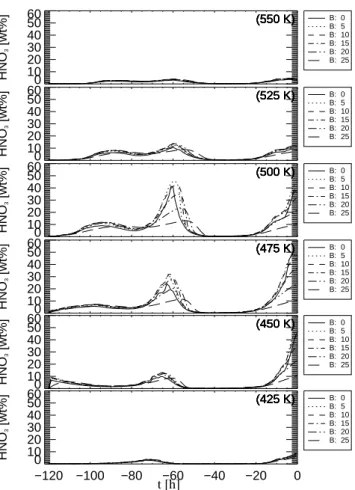
0 10 20 30 40 50 60 HNO 3 [wt%] (550 K) (550 K) (550 K) (550 K) (550 K) (550 K) B: 0 B: 5 B: 10 B: 15 B: 20 B: 25 0 10 20 30 40 50 60 HNO 3 [wt%] (525 K) (525 K) (525 K) (525 K) (525 K) (525 K) B: 0 B: 5 B: 10 B: 15 B: 20 B: 25 0 10 20 30 40 50 60 HNO 3 [wt%] (500 K) (500 K) (500 K) (500 K) (500 K) (500 K) B: 0 B: 5 B: 10 B: 15 B: 20 B: 25 0 10 20 30 40 50 60 HNO 3 [wt%] (475 K) (475 K) (475 K) (475 K) (475 K) (475 K) B: 0 B: 5 B: 10 B: 15 B: 20 B: 25 0 10 20 30 40 50 60 HNO 3 [wt%] (450 K) (450 K) (450 K) (450 K) (450 K) (450 K) B: 0 B: 5 B: 10 B: 15 B: 20 B: 25 −120 −100 −80 −60 −40 −20 0 0 10 20 30 40 50 60 HNO 3 [wt%] (425 K) (425 K) (425 K) (425 K) (425 K) (425 K) B: 0 B: 5 B: 10 B: 15 B: 20 B: 25 t [h]
Fig. 6. HNO3uptake in altitudes from 2=425 K (z∼17.8 km) to
2=550 K (z∼23.3 km) in steps of 12=25 K (1z∼1 km) as sim-ulated by the microphysical box model for the trajectory ending at Esrange.
Ocean, between the eastern coast of Greenland and Iceland, the stratospheric temperatures reached 196 K and were thus above the NAT existence temperature. Fifty hours earlier, when the air masses moved from Spitzbergen via the north-ern part of Greenland to the southnorth-ern part of Greenland, the temperature was below the STS formation temperature. Dur-ing the earliest 20 h of the trajectory temperatures were above the STS formation temperature and also above the NAT exis-tence temperature. The ice formation temperature was never reached along the 5-day trajectory.
The simulation shows that about 20 h before the observa-tion the HNO3 uptake occurred and STS particles began to form. Smaller particles grew faster than larger particles and the growth rate above ALOMAR was also larger than that above Esrange, due to colder temperatures. The final par-ticle size distribution of r∼270 nm, σ ∼1.2, and N∼8 cm−3 corresponds quite well with the lidar observations, although the distribution widths differ slightly. This can be caused by the values used for the model initialisation which we have taken from literature, since no simultaneous measurements are available. The background aerosol distribution has been
taken from Larsen et al. (2004), who measured it with an optical particle counter during similar meteorological condi-tions in the polar vortex. The HNO3and H2O values have been assumed to agree with the general background condi-tions (e.g. Meilinger et al., 1995). Smaller size distribution of the background aerosol may occur within the isolated air of the polar vortex, as a consequence of longer sedimentation time. Also, larger HNO3values may lead to stronger growth rates and finally result in even narrower size distributions of the STS particles.
An earlier HNO3uptake had occurred about 100–50 h be-fore observation, where the HNO3concentration in the PSC reached higher values for the ALOMAR trajectory than for the Esrange trajectory, since the atmospheric temperatures for the ALOMAR trajectory were slightly colder than those for the Esrange trajectory. However, between these two pe-riods with the HNO3 uptake, the atmospheric temperature increased and STS particles disappeared again. The model simulations for trajectories ending at Esrange on other alti-tudes showed a similar behaviour (see Fig. 6). In the altitude region from 19.3 km (2=450 K) to 21.5 km (2=500 K) the HNO3mass fraction reached several 10 weight percent, de-pending on particle size. This correlates very well with the altitude range of the STS layer of the mean PSC above Es-range (see Fig. 1). At 17.8 km (2=425 K) the HNO3uptake was very small with about 5 weight percent. At this alti-tude the lidars do not see any PSC. Above the STS layer, at 22.5 km (2=525 K) the HNO3 content of the particles re-duces to about 10 weight percent, which corresponds to the lidar observation of the mixed PSC layer. At higher altitudes (23.3 km or 550 K and 24.1 km or 575 K) the model calcu-lates a very limited HNO3uptake of less than 3 weight per-cent. In this altitude the lidar does not see any PSC signature.
4 Discussion
The large cross-correlation coefficient between the lidar mea-surements on both sides of the mountains, together with the good agreement between the measurements and the simu-lations, indicates that the observed PSC existed due to low temperatures on a synoptic scale. Orographically induced gravity waves which frequently cause PSC above Esrange have not influenced the PSC observation as the meteoro-logical data show. The zonal wind near the ground at Es-range, as well as at ALOMAR, is between 5 and 10 m/s at 12:00 and 18:00 UT on 5 January and even below 5 m/s at 00:00 UT on 6 January (Fig. 7), which is quite low for grav-ity wave excitation (cf. D¨ornbrack et al., 2001). Further, the zonal wind direction reverses twice with increasing altitude, which creates critical level filtering and thus effectively pre-vents orographically induced gravity waves from propagat-ing vertically into the stratosphere (e.g. Fritts and Alexander, 2003). Additionally, temperature profiles derived from the li-dar measurements in the aerosol-free part of the atmosphere
0 5 10 15 20 25 30 -10 0 10 20 30 zonal wind / m/s altitude / km Esrange 12 UT 18 UT 00 UT 0 5 10 15 20 25 30 -10 0 10 20 30 Alomar 12 UT 18 UT 00 UT
Fig. 7. ECMWF T106 zonal wind profiles for 12:00 UT (red line),
18:00 UT (green line) on 5 January and for 00:00 UT (blue line) on 6 January 2005 above Esrange (left) and ALOMAR (right). The eastward wind has a positive sign.
15 17 19 21 23 01 time / UT 16 18 20 22 24 26 a ltit u d e / k m 1.0 1.3 1.5 1.8 2.0 2.3 2.5 2.8 3.0 backsca tte r r a tio measurements
Fig. 8. Development of PSC signal above Esrange in the
perpen-dicular polarisation channel. The abscissa gives the time in UT, the ordinate the altitude in km and the colour code the backscatter ratio R. The integration time of the individual profiles is about 1 h. The start time of each profile is marked by an asterisk.
(i.e. above 30 km altitude) show very small wave perturba-tions.
In contrast to the meteorological conditions which are not favourable for gravity wave excitation and propagation, the observed PSC at Esrange shows clear wave structures with downward phase propagation. Figure 8 shows the devel-opment of the backscatter ratio in the perpendicular polar-isation channel of the U. Bonn lidar. The integration time of the individual profiles is about 1 h and the starting time of each profile is marked at the top of the figure by an as-terisk. From this observation we derived the wave param-eters vertical wavelength λz≈2.4 km and vertical phase
ve-locity cph,z≈0.11 m/s. Thus, the observed wave period is
Tobs=λz/cph,z≈6.1 h. Assuming a Brunt-V¨ais¨al¨a period of
0 5 10 15 20 25 30 -10 0 10 20 30 40 altitude / km zonal wind / m/s Iceland (65 N, 12 W) 5 January 2005 00 UT 06 UT 12 UT 0 5 10 15 20 25 30 -40 -30 -20 -10 0 10 West Greenland (79 N, 70 W) 3 January 2005 00 UT 06 UT 12 UT 0 5 10 15 20 25 30 -40 -30 -20 -10 0 10 North Greenland (83 N, 55 W) 3 January 2005 00 UT 06 UT 12 UT
Fig. 9. ECMWF T106 zonal wind data for Iceland on 5 January
2005, the western coast of northern Greenland, and the northern coast of northern Greenland on 3 January 2005. There are no critical levels above Iceland and Western Greenland and thus vertical wave propagation is not inhibited.
TBV≈5 min and using the simplified dispersion relation for
gravity waves, we can estimate the horizontal wavelength to be λx=λz×Tobs/TBV≈180 km. These parameters agree well
with gravity wave characteristics. The temporal development of the PSC in the parallel channel is essentially the same. Only between 19:00 and 23:00 UT, is the top layer of the cloud missing, which is the pure NAT layer. Thus, the wave structure exists in both solid and liquid cloud particles. Due to the short observation time at ALOMAR a similar analysis for those data is not possible.
Obviously the observed air masses experienced modula-tion due to gravity waves, however, this gravity wave in-fluence must have occurred before the air masses reached northern Scandinavia and cannot be generated locally at Es-range. The temperature back-trajectories (Fig. 5) show two possible periods when the temperatures were cold enough for STS formation. During these periods the air parcels crossed three regions where gravity waves can have been in-duced orographically. This was about 20 h before the obser-vations when the air masses were above Iceland and about 58–68 h before the observations when the air masses were between the western coast of northern Greenland and the northern coast of northern Greenland. The ECMWF T106 zonal wind data for Iceland (65◦N, 12◦W), West
Green-land (79◦N, 70◦W), and North Greenland (83◦N, 55◦W)
are shown in Fig. 9. The zonal winds at Iceland (left panel) are very strong with 10–20 m/s in the troposphere and even stronger in the stratosphere. These are very good conditions for the excitation and propagation of orographically induced gravity waves at the island of Iceland. Above the western coast of northern Greenland (centre panel) the zonal winds also support the excitation and propagation of orographically induced gravity waves, while the ground winds above the
Fig. 10. ECMWF T511 temperature map on 4 January 2005, 18:00 UT at 30 hPa (∼22 km.)
northern coast of northern Greenland (right panel) are very low close to the ground, which makes the excitation of oro-graphically induced gravity waves very unlikely. Further, close to the tropopause the zonal wind approaches zero and thus probably produces a critical level, which prevents grav-ity waves from further upward propagation.
Since the wave structure in the PSC is observable not only in the mixed part but also in the STS part of the cloud, it is more likely that the observed wave structure was induced at Iceland. A wave pattern which would have been induced al-ready at the western part of Greenland would not be observ-able any more at Esrange in the liquid part of the PSC, since the STS particles evaporated between Greenland and Ice-land and reformed again 20 h before observation in the crests where the temperature was low. Although NAT particles may have formed in the wave fields above the western part of Greenland, we assume that the solid particles at the top of the cloud have formed due to wave-induced cooling above Iceland, since this layer fits quite well within the observed wave structure. Further, the back-trajectory shows that the atmospheric temperatures have been a few Kelvin above the NAT equilibrium temperature before the air-masses reached Iceland. This indicates that NAT particles, which might have formed above Greenland, did not exist any more when the air masses reached Iceland. The atmospheric temperatures above Iceland, in the altitude region of the solid particle layer, were between TNAT and TSTS and did not fall be-low TICE the whole time covered by the back-trajectories. Since the temperature for the formation of ice clouds is about 10 K below the temperatures provided by ECMWF for Ice-land, a wave amplitude of more than 10 K is required to lead to wave-induced formation of ice PSC, which can provide condensation nuclei for heterogeneous NAT formation. The
maximum amplitude of a convectively stable temperature wave is determined by the horizontal wind, the Brunt-V¨ais¨al¨a frequency, and the adiabatic temperature gradient. This re-sults in 1T ≈14 K at 22 km altitude above Iceland, according to the respective ECMWF data. A wave amplitude of 14 K at an altitude of about 22 km or 33 hPa corresponds to a vertical excursion of 1400 m, assuming a dry-adiabatic temperature gradient of 10 K/km. This vertical excursion of 1400 m in the stratosphere reduces to 250 m at the ground, i.e. 1013 hPa, in the case of a non-dissipative gravity wave. The back-trajectory, which ends at Esrange, crosses the southern part of Iceland where mountains as high as 2000 m exist. Assuming a maximum temperature wave modulation of 14 K and tak-ing the assumed horizontal wavelength and the zonal wind speed in the stratosphere into account, a maximum existence time for ice particles can be estimated by the half of the nega-tive phase of this wave. This results in a maximum existence time of tex<180 km/30 ms−1/4≈25 min. This short period
can already be sufficient for heterogeneous NAT formation on ice particles, as Luo et al. (2003) show.
As the lidar temperature data from ALOMAR and Esrange indicate, there were no wave signatures at 30-km altitude and above. The wave activity measured in terms of the gravity wave potential energy density (see Blum et al., 2004, for de-tails) was about one order of magnitude lower during the measurements than the average winter values. Radiosonde data from Bodø and Sodankyl¨a support this observation. In the radiosonde data there are no wave signatures above the tropopause. Since there were no critical levels above the PSC altitude, we can assume that the observed wave structure in the PSC is not caused by a wave-like temperature modula-tion above Esrange. Rather, we have to assume that the wave structure was “frozen” in the PSC and then advected by the background wind. High resolution ECMWF T511 analyses also do not show any wave activity during the lidar observa-tions on 5 January 2005 within the whole polar vortex, how-ever, about 24 h earlier strong wave activity between Iceland and Scandinavia existed (see Fig. 10). On 4 January 2005, at 18:00 UT, the horizontal wavelength in the ECMWF T511 analysis at 30 hPa (∼22 km) is about 200 km and the temper-ature amplitude about 5–10 K. This wave field is more pro-nounced at northern Scandinavia than at Iceland, however, it agrees quite well with the wave parameters derived from the lidar measurements. Although all estimates for the gravity wave amplitude near 22 km altitude allow for ice formation, there is no measurement of the actual temperature reached in the wave crests and it is possible that ice particles were not formed. While our observations are compatible with the scenario that NAT formation processes via nucleation on ice, it is possible that other condensation nuclei may have been involved (e.g. Bogdan and Kulmala, 1999).
5 Summary
On 5 January 2005 the U. Bonn lidar at Esrange, as well as the ALOMAR RMR and O3-lidar, simultaneously ob-served a polar stratospheric cloud which we classified as STS in the lower part and a mixture of solid and liquid parti-cles (STS and NAT) in the upper part of the cloud. Micro-physical model calculations, coupled with temperature his-tories showed that the STS particles formed about 20 h be-fore the observations. The uptake of HNO3 was modeled in the altitude range where the lidar observed the STS layer. Very narrow particle size distributions were observed by li-dar and found by the model simulations with similar param-eters. A reduced HNO3uptake was modelled in the altitude of the mixed layer. Cross-correlation calculations revealed that the shape of the observed cloud was extremely similar on both sides of the Scandinavian mountains (CCF=88.3%) and meteorological conditions were not favourable for oro-graphic gravity wave excitation and vertical propagation, nei-ther above Esrange nor above ALOMAR. This indicates that the PSC existed due to synoptically cold temperatures. The observed wave structure in the cloud was probably induced above Iceland and advected to northern Scandinavia. Strong ground winds at Iceland may have excited orographically-induced gravity waves and critical levels did not exist. Thus excellent excitation and propagation conditions for gravity waves existed above Iceland. The solid particles fit well in the wave pattern and thus should have formed together with the STS particles of the cloud. Large wave amplitudes of more than 10 K must have been reached for the formation of ice particles which can serve as condensation nuclei for NAT. Although such large wave amplitudes are close to the wave amplitude saturation limit of 14 K, a heterogeneous for-mation of the solid particles on ice is possible, since the air masses can have experienced such cold temperatures for a sufficiently long time in the wave field above Iceland. How-ever, it is not clear from the data whether the NAT particles have formed on ice or on other condensation nuclei, such as meteoric dust.
Acknowledgements. We thank the staffs of Esrange and Andøya Rocket Range for their always quick and uncomplicated support during the measurement campaign. Further, we thank V. Alishahi and N. Thomas for their help calculating the air parcel trajectories. We are also thankful to P. Deuflhard and U. Nowak for provid-ing the solver for ordinary differential equations and to M. Hervig for providing a program to calculate the NAT existence tempera-ture TNAT. The measurements at Esrange were funded by the
En-visat Validation project granted by the DLR Erdbeobachtung FKZ 50 EE 0009. The measurements at ALOMAR were supported by the Transnational Access to Research Infrastructure under the EU’s 6. FP. U. Blum and F. Khosrawi are supported by the Marie-Curie Intra-European Fellowship programme of the European Com-munity (No. 010333, MINERWA; No. 515292, FAST). Finally, U. Blum and F. Khosrawi are grateful to the organisers of the NorFA graduate school on Middle Atmospheric Aerosols (J. Gumbel and M. Rapp) where the contact was established that led to this
collab-oration. The ALOMAR Ozone lidar is owned and operated by the Norwegian Defence Research Establishment (FFI), the Norwegian Institute for Air Research (NILU), and Andøya Rocket Range.
Topical Editor U.-P. Hoppe thanks two referees for their help in evaluating this paper.
References
Blum, U. and Fricke, K. H.: The Bonn University Lidar at the Es-range: Technical description and capabilities for atmospheric re-search, Ann. Geophys., 23, 1645–1658, 2005,
http://www.ann-geophys.net/23/1645/2005/.
Blum, U., Fricke, K. H., Baumgarten, G., and Sch¨och, A.: Simulta-neous lidar observations of temperatures and waves in the polar middle atmosphere on the east and west side of the Scandinavian mountains: a case study on 19/20 January 2003, Atmos. Chem. Phys., 4, 809–816, 2004,
http://www.atmos-chem-phys.net/4/809/2004/.
Blum, U., Fricke, K. H., M¨uller, K.-P., Siebert, J., and Baumgarten, G.: Long-term lidar observations of polar stratospheric clouds at Esrange in northern Sweden, Tellus, 57B, 412–422, 2005. Bogdan, A. and Kulmala, M.: Aerosol silicia as a possible
candi-date for the heterogeneous formation of nitric acid hydrates in the stratosphere, Geophys. Res. Lett., 26, 1433–1436, 1999. Browell, E. V., Butler, C. F., Ismail, S., Robinette, P. A., Carter,
A. F., Higdon, N. S., Toon, O. B., Schoeberl, M. R., and Tuck, A. F.: Airborne lidar observations in the wintertime Arctic strato-sphere: Polar stratospheric clouds, Geophys. Res. Lett., 17, 385– 388, 1990.
Carslaw, K. S., Luo, B. P., Clegg, S. L., Peter, T., Brimblecombe, P., and Crutzen, P. J.: Stratospheric aerosol growth and HNO3gas
phase depletion from coupled HNO3and water uptake by liquid
particles, Geophys. Res. Lett., 21, 2479–2482, 1994.
Carslaw, K. S., Peter, T., and Clegg, S. L.: Modeling the composi-tion of liquid stratospheric aerosols, Rev. Geophys., 35, 125–154, 1997.
Carslaw, K. S., Peter, T., Bacmeister, J. T., and Eckermann, S. D.: Widespread solid particle formation by mountain waves in the Arctic stratosphere, J. Geophys. Res., 104, 1827–1836, 1999. Crutzen, P. and Arnold, F.: Nitric acid cloud formation in the cold
Antarctic stratosphere: A major cause for springtime ‘ozone hole’, Nature, 324, 651–655, 1986.
D¨ornbrack, A., Leutbecher, M., Reichardt, J., Behrend, A., M¨uller, K.-P., and Baumgarten, G.: Relevance of mountain wave cooling for the formation of polar stratospheric clouds over Scandinavia: Mesoscale dynamics and observations for January 1997, J. Geo-phys. Res., 106, 1569–1581, 2001.
Fritts, D. C. and Alexander, M. J.: Gravity wave dynamics and effects in the middle atmosphere, Rev. Geophys., 41(1), 1003, doi:10.1029/2001RG000106, 2003.
Hanson, D. and Mauersberger, K.: Laboratory studies of the ni-tric acid trihydrate: Implications for the south polar stratosphere, Geophys. Res. Lett., 15, 855–858, 1988.
Hedin, A. E.: Neutral atmosphere empirical model from the surface to the lower Exosphere MSISE90, J. Geophys. Res., 96, 1159– 1172, 1991.
Hoppe, U.-P., Hansen, G., and Opsvik, D.: Differential absorption lidar measurements of stratospheric ozone at ALOMAR: First results, Proceedings of the 12th ESA Symposium on European
Rocket and Ballon Programmes and Related Research, Lilleham-mer, Norway, ESA-SP-370, 335–344, 1995.
Jin, J. J., Semeniuk, K., Manney, G. L., Jonsson, A. I., Bea-gley, S. R., McConnell, J. C., Dufour, G., Nassar, R., Boone, C. D., Walker, K. A., Bernath, P. F., and Rinsland, C. P.: Severe Arctic ozone loss in the winter 2004/2005: Observa-tions from ACE-FTS, Geophys. Res. Lett., 33(15), L15801, doi:10.1029/2006GL026752, 2006.
Khosrawi, F. and Konopka, P.: Enhancement of nucleation and con-densation rates due to mixing in the tropopause region, Atmos. Environ., 37, 903–910, 2003.
Knopf, D. A., Koop, T., Luo, B. P., Weers, U. G., and Peter, T.: Homogeneous nucleation of NAD and NAT in liquid stratosphere aerosols: Insufficient to explain denitrification, Atmos. Chem. Phys., 2, 207–214, 2002,
http://www.atmos-chem-phys.net/2/207/2002/.
Krieger, U. K., M¨osinger, J. C., Luo, B., Weers, U., and Peter, T.: Measurement of the refractive indices of H2SO4-HNO3-H2O
so-lutions to stratospheric temperatures, Appl. Opt., 39, 3691–3703, 2000.
Larsen, N., Knudsen, B. M., Svendsen, S. H., Deshler, T., Rosen, J. M., Kivi, R., Weisser, C., Schreiner, J., Mauersberger, K., Cairo, F., Ovarlez, J., Oelhaf, H., and Spang, R.: Formation of solid particles in synoptic-scale Arctic PSCs in early winter 2002/2003, Atmos. Chem. Phys., 4, 2001–2013, 2004,
http://www.atmos-chem-phys.net/4/2001/2004/.
Luo, B. P., Carslaw, K. S., Peter, T., and Clegg, S. L.: Vapour pres-sures of H2SO4/HNO3/HCl/HBr/H2O solutions to low strato-spheric temperatures, Geophys. Res. Lett., 22, 247–250, 1995. Luo, B. P., Voigt, C., Flueglistaler, S., and Peter, T.:
Ex-treme NAT supersaturation in mountain wave ice PSCs: A clue to NAT formation, J. Geophys. Res., 108, 4441, doi:10.1029/2002JD003104, 2003.
MacKenzie, A. R.: On the theories of type 1 polar stratospheric cloud formation, J. Geophys. Res., 100, 11 275–11 288, 1995. Marti, J. and Mauersberger, K.: A survey and new measurements
of ice vapor pressure temperatures between 170 and 250 K, Geo-phys. Res. Lett., 20, 363–366, 1993.
McCormick, M. P., Steele, H. M., Hamill, P., Chu, W. P., and Swissler, T. J.: Polar stratospheric cloud sightings by SAM II, J. Atmos. Sci., 39, 1387–1397, 1982.
McKenna, D. S., Konopka, P., Grooß, J.-U., G¨unther, G., M¨uller, R., Spang, R., Offermann, D., and Orsolini, Y.: A new Chemi-cal Lagrangian Model of the Stratosphere (CLaMS): Part I For-mulation of advection and mixing, J. Geophys. Res., 107, 4309, doi:10.1029/2000JD000114, 2002.
Meilinger, S., Koop, K., Luo, B. P., Huthwelker, T., Carslaw, K. S., Krieger, U., Crutzen, P. J., and Peter, T.: Size-dependent strato-spheric droplet composition in lee wave temperature fluctuations and their potential role in PSC freezing, Geophys. Res. Lett., 22, 3031–3034, 1995.
Mishchenko, M. I., Hovenier, J. W., and Travis, L. D.: Light scatter-ing by nonspherical particles, Academic Press, San Diego, 1999. Mishchenko, M. I., Travis, L. D., and Lacis, A. A.: Scattering, absorption, and emission of light by small particles, Cambridge University Press, Cambridge, 2002.
Peter, T.: Microphysics and heterogeneous chemistry of polar stratospheric clouds, Ann. Rev. Phys. Chem., 48, 785–822, 1997. Poole, L. R. and McCormick, M. P.: Airborne lidar observations
of Arctic polar stratospheric clouds: Indications of two distinct growth stages, Geophys. Res. Lett., 15, 21–23, 1988.
Pruppacher, H. and Klett, J. D.: Microphysics of clouds and precip-itation, D. Reidel, Norwell, Mass., 1978.
Rex, M., Salawitch, J., von der Gathen, P., Harris, N. R., Chipperfield, M. P., and Naujokat, B.: Arctic ozone loss and climate change, Geophys. Res. Lett., 31, L04116, doi:10.1029/GL018844, 2004.
Solomon, S.: Stratospheric ozone depletion: A review of concepts and history, Rev. Geophys., 37, 275–316, 1999.
Solomon, S., Garcia, R. R., Rowland, F. S., and Wuebbles, D. J.: On the depletion of Antarctic ozone, Nature, 321, 755–758, 1986. Steele, H. M., Hamill, P., McCormick, M. P., and Swissler, T. J.:
The formation of polar stratospheric clouds, J. Atmos. Sci., 40, 2055–2067, 1983.
Stetzer, O., M¨ohler, O., Wagner, R., Benz, S., Saathoff, H., Bunz, H., and Indris, O.: Homogeneous nucleation rates of nitric acid dihydrate (NAD) at simulated stratospheric conditions – Part I: Experimental results, Atmos. Chem. Phys., 6, 3023–3033, 2006, http://www.atmos-chem-phys.net/6/3023/2006/.
Tabazadeh, A., Turco, R. P., Drdla, K., and Jacobsen, M. Z.: A study of type I polar stratospheric cloud formation, Geophys. Res. Lett., 21, 1619–1622, 1994.
Tabazadeh, A., Jensen, E. J., Toon, O. B., Drdla, K., and Schoeberl, M. R.: Role of the stratospheric polar freezing belt in denitrifica-tion, Science, 291, 2591–2594, 2001.
Tilmes, S., M¨uller, R., Grooß, J.-U., and Russell, J. M.: Ozone loss and chlorine activation in the Arctic winters 1991–2003 derived with the tracer-tracer correlations, Atmos. Chem. Phys., 4, 2181– 2213, 2004,
http://www.atmos-chem-phys.net/4/2181/2004/.
Tilmes, S., M¨uller, R., Engel, A., Rex, M., and Russel III, J. M.: Chemical ozone loss in the Arctic and Antarctic stratosphere between 1992 and 2005, Geophys. Res. Lett., 33, L20812, doi:10.1029/2006GL026925, 2006.
Voigt, C., Schreiner, J., Kohlmann, A., Zink, P., Mauersberger, K., Larsen, N., Deshler, T., Kr¨oger, C., Rosen, J., Adriani, A., Cairo, F., Donfrancesco, G. D., Viterbini, M., Ovarlez, J., David, C., and D¨ornbrack, A.: Nitric Acid Trihydrate (NAT) in polar strato-spheric clouds, Science, 290, 1756–1758, 2000.
Voigt, C., Schlager, H., Luo, B. P., D¨ornbrack, A., Roiger, A., Stock, P., Curtius, J., V¨ossing, H., Borrman, S., Davies, S., Konopka, P., Schiller, C., Shur, G., and Peter, T.: Nitric acid trihydrate (NAT) formation at low NAT supersaturation in polar stratospheric clouds (PSCs), Atmos. Chem. Phys., 5, 1371–1380, 2005,
http://www.atmos-chem-phys.net/5/1371/2005/.
Volkert, H. and Intes, D.: Orographically forced stratospheric waves over northern Scandinavia, Geophys. Res. Lett., 19, 1205–1208, 1992.
von Hobe, M., Ulanovsky, A., Volk, C. M., Grooß, J.-U., Tilmes, S., Konopka, P., G¨unther, G., Werner, A., Spelten, N., Shur, G., Yushkov, V., Ravegnani, F., Schiller, C., M¨uller, R., and Stroh, F.: Severe ozone depletion in cold Arctic winter 2004–05, Geophys. Res. Lett., 33(17), L17815, doi:10.1029//2006GL026945, 2006. von Zahn, U., von Cossart, G., Fiedler, J., Fricke, K. H., Nelke, G., Baumgarten, G., Rees, D., Hauchecorne, A., and Adolfsen, K.: The ALOMAR Rayleigh/Mie/Raman lidar: Objectives, configu-ration, and performance, Ann. Geophys., 18, 815–833, 2000,
http://www.ann-geophys.net/18/815/2000/.
Worsnop, D. R., Fox, L. E., Zahniser, M. S., and Wofsy, S. C.: Vapor pressures of solid hydrates of nitric acid: Implications for polar stratospheric clouds, Science, 259, 71–74, 1993.
Young, A. T.: Revised depolarization corrections for atmospheric extinction, Appl. Opt., 19, 3427–3428, 1980.