HAL Id: hal-00318145
https://hal.archives-ouvertes.fr/hal-00318145
Submitted on 13 Sep 2006
HAL is a multi-disciplinary open access
archive for the deposit and dissemination of
sci-entific research documents, whether they are
pub-lished or not. The documents may come from
teaching and research institutions in France or
abroad, or from public or private research centers.
L’archive ouverte pluridisciplinaire HAL, est
destinée au dépôt et à la diffusion de documents
scientifiques de niveau recherche, publiés ou non,
émanant des établissements d’enseignement et de
recherche français ou étrangers, des laboratoires
publics ou privés.
Stratospheric and mesospheric temperature variations
for the quasi-biennial and semiannual (QBO and SAO)
oscillations based on measurements from SABER
(TIMED) and MLS (UARS)
F. T. Huang, H. G. Mayr, C. A. Reber, J. M. Russell, M. Mlynczak, J. G.
Mengel
To cite this version:
F. T. Huang, H. G. Mayr, C. A. Reber, J. M. Russell, M. Mlynczak, et al.. Stratospheric and
mesospheric temperature variations for the quasi-biennial and semiannual (QBO and SAO) oscillations
based on measurements from SABER (TIMED) and MLS (UARS). Annales Geophysicae, European
Geosciences Union, 2006, 24 (8), pp.2131-2149. �hal-00318145�
www.ann-geophys.net/24/2131/2006/ © European Geosciences Union 2006
Annales
Geophysicae
Stratospheric and mesospheric temperature variations for the
quasi-biennial and semiannual (QBO and SAO) oscillations based
on measurements from SABER (TIMED) and MLS (UARS)
F. T. Huang1, H. G. Mayr2, C. A. Reber2, J. M. Russell3, M Mlynczak4, and J. G. Mengel5
1Creative Computing Solutions Inc., Rockville, MD 20850, USA 2NASA Goddard Space Flight Center, Greenbelt MD, 20771, USA
3Hampton University, Center for Atmospheric Sciences, Hampton, VA, 23668, USA 4NASA Langley Research Center, Hampton, VA, 23681, USA
5Science Systems and Applications, Lanham, MD, 20706, USA
Received: 28 February 2006 – Revised: 5 July 2006 – Accepted: 17 July 2006 – Published: 13 September 2006
Abstract. We present the zonal mean temperature variations
for the quasi-biennial oscillation (QBO) and the semiannual oscillation (SAO) based on data from SABER on the TIMED spacecraft (years 2002 to 2004) and from MLS on the UARS mission (1992 to 1994). The SABER measurements pro-vide the rare opportunity to analyze data from one instru-ment over a wide altitude range (15 to 95 km), while MLS data were taken in the 16 to 55 km altitude range a decade earlier. The results are presented for latitudes from 48◦S to 48◦N. New results are obtained for the QBO, especially in the upper stratosphere and mesosphere, and at mid-latitudes. At Equatorial latitudes, the QBO amplitudes show local peaks, albeit small, that occur at different altitudes. From about 20 to 40 km, and within about 15◦of the Equator, the amplitudes can approach 3.5◦K for the stratospheric QBO (SQBO). For the mesospheric QBO (MQBO), we find peaks near 70 km, with temperature amplitudes reaching 3.5◦K, and near 85 km, the amplitudes approach 2.5◦K. Morpho-logically, the amplitude and phase variations derived from the SABER and MLS measurements are in qualitative agree-ment. As a function of latitude, the QBO amplitudes tend to peak at the Equator but then increase again pole-ward of about 15◦ to 20◦. The phase progression with altitude varies more gradually at the Equator than at mid-latitudes. Many of the SAO results presented are also new, in part be-cause measurements were not previously available or were more limited in nature. At lower altitudes near 45 km, within about 15◦of the Equator, the temperature amplitudes for the stratospheric SAO (SSAO) reveal a local maximum of about 5◦K. At higher altitudes close to the Equator, our results show separate peaks of about 7◦K near 75 and 90 km for the mesospheric SAO (MSAO). In the SAO results, significant inter-annual differences are evident, with the amplitudes be-ing largest in 2002 relative to 2003 and 2004. As in the case Correspondence to: F. T. Huang
(fthuang@comcast.net)
for the QBO, the SAO temperature amplitudes go through minima away from the Equator, and then increase towards mid latitudes, especially at altitudes above 55 km. We com-pare our findings with previously published empirical results, and with corresponding results from the numerical spectral model (NSM). Although not a focus of this study, we also show results for the inter-annual variations (which appear to be generated at least in part by the QBO) of the migrating diurnal tide. In the upper mesosphere, their amplitudes can approach 20◦K, and they are derived jointly with the zonal-mean components.
Keywords. Meteorology and atmospheric dynamics
(Mid-dle atmosphere dynamics; Thermospheric dynamics) – At-mospheric composition and structure (Pressure, density, and temperature)
1 Introduction
The zonal-mean temperature variations of the Semi-annual Oscillation (SAO) and Quasi-biennial Oscillation (QBO) in the stratosphere and mesosphere are produced mainly by dy-namical processes, which are associated with the zonal cir-culation that dominates at, and is confined to equatorial lati-tudes. In this respect, the dynamical situation is similar to the one that controls the temperature variations of the dominant Annual Oscillation (AO) in the mesosphere at high latitudes (Lindzen, 1981), in contrast to the stratospheric AO, which is generated primarily by solar heating.
At low latitudes, the zonal mean zonal winds of the SAO peak in the upper stratosphere near 50 km with velocities of about 30 m/s, eastward during equinox and westward around solstice (e.g., Hirota, 1980). In the upper mesosphere near 80 km, a second peak is observed with comparable magni-tude but opposite phase.
2132 F. T. Huang et al.: Stratospheric and mesospheric temperature variations The zonal mean zonal wind QBO is observed in the lower
stratosphere with a maximum at around 30 km, having am-plitudes close to 20 m/s (e.g., Reed, 1965, 1966). Such os-cillations, with opposite phases, have been inferred also for the upper mesosphere (Burrage et al., 1996) based on mea-surements with the HRDI instrument on UARS (Hays et al., 1993).
Lindzen and Holton (1968) and Holton and Lindzen (1972) established that wave-mean flow interactions can gen-erate a QBO. They invoked equatorially trapped planetary waves (i.e., eastward propagating Kelvin waves and west-ward propagating Rossby gravity waves) to provide the wave forcing through critical level absorption and radiative damp-ing. Plumb (1977), Plumb and Bell (1982) and Dunkerton (1985a), and others, further elucidated the properties of this mechanism. With the Sun crossing the equator twice a year, a semi-annual oscillation is generated through momentum ad-vection from the summer to the winter hemisphere. The mag-nitude of this oscillation is small compared with observations (e.g., Meyer, 1970; Hamilton, 1986), and the theory for the QBO by Lindzen and Holton was therefore extended to also explain the SAO in the stratosphere (e.g., Dunkerton, 1979; Hamilton, 1986, Hitchman and Leovy, 1986). The planetary waves that are postulated to drive the equatorial oscillations in the stratosphere are largely dissipated there, and therefore cannot significantly affect the dynamics of the upper meso-sphere. Lindzen (1981) had shown that in this region of the atmosphere, at higher altitudes, small-scale gravity waves (GW) can cause the seasonal variations of the zonal circula-tion to reverse; and Dunkerton (1982a) proposed this mech-anism to explain the observed SAO above 70 km. Hitchman and Leovy (1986) provide a good discussion of the dynam-ical processes that generate the SAO in the stratosphere and mesosphere. They also discussed specifically the important role of the gravity-wave-driven meridional circulation.
During the last decade, the importance of GWs relative to planetary waves in the middle atmosphere has been in-creasingly recognized. From a modeling study, Hitchman and Leovy (1988) concluded that the observed Kelvin waves, based on data from the Limb Infrared Monitor of the Strato-sphere (LIMS) instrument (Nimbus 7 satellite), can account for only 20%–70% of the stratospheric SAO and that GWs are likely to be important too. With a general circulation model (GCM) that resolves planetary waves but not GWs, Hamilton et al. (1995) showed that the observed eastward phase of the stratospheric SAO cannot be simulated and that the amplitude of the QBO is almost an order of magnitude smaller than observed, suggesting again that GWs are play-ing a more prominent role. Except for a few attempts at sim-ulating the zonal winds of the QBO and SAO with resolved GWs (e.g., Takahashi, 1999), these waves need to be param-eterized for global-scale models. Following Lindzen (1981), the parameterization of GW interactions with the background flow thus has been the subject of numerous studies (e.g., Dunkerton, 1982b, c, 1987; Fritts and Lu, 1993; Hines,
1997a, b). The Doppler Spread Parameterization (DSP) of Hines (1997a, b) for example, which deals with a spectrum of waves and accounts both for wave-wave and wave-mean-flow interactions, has been applied successfully in several models (e.g., Mengel et al., 1995; Mayr et al., 1997; Manzini et al., 1997; Akmaev, 2001; McLandress, 1998, 2002).
An important property of the QBO is that the observed confinement of the zonal winds to equatorial latitudes can be simulated even with a wave source that is globally uniform (e.g., Mengel et al., 1995). At the equator where the Coriolis force vanishes, the waves accelerate the zonal winds without generating a meridional circulation that would tend to redis-tribute and dissipate the flow momentum. The flow thus is essentially trapped around the equator, where the wave in-teraction is primarily balanced by eddy viscosity causing the QBO to propagate down. Away from the equator, irrespec-tive of the wave source, the meridional circulation comes into play and dissipates the zonal flow (e.g., Haynes, 1998). With-out the meridional circulation, the QBO zonal winds at the equator could be described for simplicity with a one dimen-sional “prototype model”, as Lindzen and Holton (1968) had pointed out.
Holton and Tan (1980) showed how the wave-driven QBO can affect the temperature variations at high latitudes, and in several subsequent papers (e.g., Labitzke, 1982, 1987; Lab-itzke and van Loon, 1988, 1992) the processes involved were further explored. While the subordinate role of the merid-ional circulation near the equator explains the essential prop-erties of the zonal winds that characterize the QBO, and the SAO to a lesser extent, the dynamical situation is virtually reversed for the related temperature variations. The merid-ional circulation that dissipates the QBO zonal winds away from the equator produce temperature oscillations that ex-tend to high latitudes, and in the mesosphere in particular, as shown in 2-D models (e.g., Mayr et al., 2000). Temperature observations thus can provide valuable information bearing on the configuration of the meridional circulation, which in turn depends on the latitude dependence of the wave forcing that generates the QBO and SAO.
In the following, we present results from an analy-sis of temperature data obtained from the Thermosphere-Ionosphere-Mesosphere-Energetics and Dynamics (TIMED) satellite and from the Upper Atmosphere Research Satellite (UARS, Reber, 1993). The measurements were carried out on TIMED by the Sounding of the Atmosphere using Broad-band Emission Radiometry (SABER) instrument (Russell et al., 1999), and on UARS by the Microwave Limb Sounder (MLS, Barath et al., 1993). The data are analyzed to derive the zonal-mean temperature variations for the QBO and SAO from 15 to 95 km altitude and from 48◦S to 48◦N latitude.
Our results are compared with those obtained from other satellites, sounding rockets, and ground-based observations. We also compare them with recent results from the Numeri-cal Spectral Model (Mayr and Mengel, 2005).
Within about 15◦ of the Equator, our results for both the QBO and SAO show that there are small local peaks in amplitudes as a function of altitude. For the QBO in the mesosphere (MQBO), there are separate peaks near 70 and 85 km. In the stratosphere (SQBO), the amplitudes are broadly larger from about 20 to 40 km. Although the am-plitudes tend to decrease away from the Equator, pole-ward of about 20◦ latitude, the amplitudes can recover to larger values, depending on the altitude. The phase variations with altitude are quite different at low latitudes compared to those at mid-latitudes. For the equatorial SAO, there are peaks in amplitude near 45 km, corresponding to the strato-sphere semiannual oscillation (SSAO), and separate peaks near 75 and 90 km, corresponding to the mesospheric oscil-lation (MSAO). As with the QBO, the SAO amplitudes tend to decrease away from the Equator, but can increase at higher latitudes, especially above about 55 km.
Although thermal tides are not the focus of this study, their variations are embedded in the data, can be significant, and cannot be ignored. The tidal variations need to be unrav-eled from the mean variations in the data in order to obtain more accurate estimates of both. In addition to the zonal-mean components, it is thus important that our analysis also accounts for the seasonal and inter-annual temperature vari-ations of the diurnal tides, and we present some results for that as well.
2 Satellite data, sampling, and analysis
TIMED was launched at the end of 2001, and we analyzed the SABER temperature data for years 2002 through 2004, in the altitude range from 15 to 95 km. UARS was launched in September 1991, and the MLS data were analyzed for 1992 and 1993, from 100 to 1 hPa (about 16 to 48 km). The SABER and MLS instruments both measure the emitted radi-ation as they view the Earth’s limb, and the temperatures are retrieved by applying radiative transfer analysis. The data are sampled at different latitudes because of the north/south motion of the satellites, and different longitudes are sampled due to the rotation of the Earth relative to the orbital plane. It takes up to one day to sample the data over the globe, so global measurements are not obtained simultaneously. The SABER project supplies level 2 data (version 1.4), which represent the measurements at the footprints of the instru-ment as a function of space and time. We interpolated the data to fixed altitude surfaces and latitudes. They were then averaged over longitude for the analysis. Our analyses are made at altitude intervals of 2.5 km (close to the resolution of the data) and latitude intervals of 4◦. The analyses are made independently at individual latitudes and altitudes, and are uncoupled from each other. MLS provides level 3 data at regular latitudes and pressure surfaces.
On any given day, irrespective of longitude, satellites usu-ally sample the data at only two local solar times around a
lat-itude circle, one for the ascending (north bound) orbit mode, and one for the descending mode. For sun-synchronous satel-lites, the two local times remain the same throughout the mission, making it impractical to quantitatively analyze vari-ations as a function of local time.
Unlike sun-synchronous satellites, the orbital planes of TIMED and UARS precess slowly due to the respective or-bital inclinations of 74◦and 57◦. Because the orbital preces-sion is slow, SABER and MLS also sample essentially only at one local solar time (corresponding to each orbital mode) during a given day, around a given latitude circle. Therefore, estimates of the zonal mean (average of the data around a lat-itude circle for a given day) can be biased by variations with local time. From day to day, for a given latitude and orbital mode, the local times of the measurements decrease by about 12 and 20 min for TIMED and UARS, respectively. Using both orbital modes, it takes 60 days for SABER and 36 days for MLS to sample the data over the full range of local times, thereby providing more information on variations with lo-cal time, compared to sun-synchronous satellites. However, over periods of 60 and 36 days, both the diurnal tides and the zonal-mean variations contribute to the observed temperature variations, and therefore they need to be separately identified. In the mesosphere and lower thermosphere for example, the temperature amplitudes of the diurnal tide (∼20◦K) can be as large as those of the zonal-mean variations. To account for the above properties of the data sampling, the algorithm employed in the analysis estimates jointly the diurnal vari-ations of the diurnal tides and the zonal mean varivari-ations as described in the appendix. Applying least square analysis to the satellite data at a given altitude and latitude, the algorithm estimates the coefficients of a two-dimensional Fourier se-ries with the independent variables being local solar time and day-of-year. For the zonal mean, the Fourier components as a function of day of year then describe the temperature varia-tions of the QBO, AO, SAO, and higher harmonics. Because of the sampling in local time described above, the analysis of data averaged over longitude produces variations with local time that correspond to migrating tides. The algorithm used here has been successfully applied previously to UARS tem-perature and wind data, and to SABER temtem-perature data, as discussed in Huang et al. (2003, 2005).
As an example of our analysis, we present in Fig. 1 the SABER temperature (◦K) data averaged over longitude and the estimated results, plotted at the Equator versus day of year for years 2002 and 2003. The upper panel (a) shows the data and analysis results at 35 km. The red and green lines show the data from the ascending and descending modes, and the diamonds and squares represent the corresponding esti-mated fit to the data. To avoid crowding, the fitted values are presented only for every 3 data points. The estimated fit is obtained by evaluating the Fourier series at the same day and same local time as the data. Note that the ascending and de-scending mode data are not very different even though they represent very different local times, reflecting the relatively
2134 F. T. Huang et al.: Stratospheric and mesospheric temperature variations
23 Figures
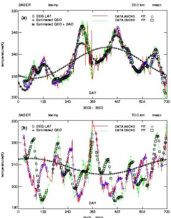
Figure 1. Zonally (longitudinally) averaged SABER temperature data and derived (estimated) analysis results plotted versus day of years 2002 - 2003 at the Equator for 35 km (a) and 70 km (b). Red line and diamonds represent ascending mode data and fit, respectively. Green line and squares represent descending mode data and fit,
respectively. Black '+' represent estimated QBO; black asterisks estimated QBO + SAO. To avoid crowding, only the QBO component is shown at 70 km where the tidal variations are large.
Fig. 1. Zonally (longitudinally) averaged SABER temperature data and derived (estimated) analysis results plotted versus day of years 2002–2003 at the Equator for 35 km (a) and 70 km (b). Red line and diamonds represent ascending mode data and fit, respectively. Green line and squares represent descending mode data and fit, re-spectively. Black “+” represent estimated QBO; black asterisks es-timated QBO + SAO. To avoid crowding, only the QBO component is shown at 70 km where the tidal variations are large.
small tidal variations. Our analysis shows that the observed temperature variations at 35 km primarily reflect that of the zonal mean, rather than the tides. This is evident from the estimates for the QBO (plus yearly mean) presented with “+” symbols and from the sum of QBO and SAO (asterisks), which are derived with our algorithm.
Analogous to Fig. 1a, we present in the lower panel (b) the data and analysis results for 70 km. At this altitude, in contrast to 35 km, the ascending and descending mode data for each day can differ significantly, by up to 20◦K, reflect-ing the larger tidal variations at different local times. As the day numbers increase, the data are sampled at local times that decrease by about 12 min each day. Since the algorithm employs a Fourier series that describes the inter-annual, sea-sonal, and inter-seasonal variations (with periods as short as two months), the derived values for each day represent a rel-atively close fit to the data, reflecting the year-long varia-tions of the tides and the zonal mean components. As in Fig. 1a, we show with “+” the estimated QBO component in
the temperature variations derived with our algorithm, which confirms that the temperature oscillations extend with signif-icant amplitudes into the upper mesosphere, as also observed in the zonal wind data from UARS (Burrage et al., 1996). The derived SAO component is even larger, but is not shown because the plot becomes “busy” and difficult to read.
Our analysis differs from that of Dunkerton and Delisi (1985b) who analyzed data from the NOAA Monthly Cli-matic Data for the World (MCDW), in which the QBO is treated as the residual after removing the annual and semian-nual components from the data. This approach works well in the lower stratosphere where the tides are weak as seen from Fig. 1a. In the upper stratosphere and mesosphere however, the QBO and SAO are derived with an analysis of the kind presented here, which accounts for the large tidal oscillations embedded in the data shown in Fig. 1b.
3 Measurement results
3.1 Zonal-mean components
3.1.1 Quasi-Biennial Oscillation (QBO)
Unlike the 6-month SAO and the 12-month AO that are closely tied to solar heating, the QBO phenomenon is char-acterized by periods (on average somewhat larger than two years), phases, and amplitudes that are not tied to the sea-sonal cycle but can vary with space and time. This makes it difficult to describe the QBO in terms of Fourier series, which are characterized by fixed periods, amplitudes, and phases. We also have only three years of data, and the statis-tics therefore are not good.
In the analysis presented here, we estimated the QBO tem-perature component by assuming periods of 22, 24, 26, 28, and 29 months. We also used a sliding window in our anal-ysis. For example, in addition to estimating the QBO from data in the year day interval 2002001 to 2003365, we have also applied the algorithm to data in the interval 2003001 to 2004365, among others. The salient features of the derived QBOs are not sufficiently different to clearly choose one riod over the others. Considering that the observed QBO pe-riod of the zonal winds in the lower stratosphere (where the oscillation originates) is close to 26 months we present re-sults by assuming a period of 26 months, and for comparison we present also some results for the 24-month QBO. That 26 months may not match the period of the QBO exactly, and that the period, amplitude, and phase may drift over a cycle, is similar to the situation where the represented sinusoids are modulated, and similar to effects of applying data windows. Effectively, these can result in leakage to adjacent frequen-cies, and smoothing in the amplitudes (Bloomfield, 1976). However, the effects are not expected to be very significant, since the actual amplitudes and phases vary relatively slowly and smoothly.
0.00 1.25 2.50 3.75 5.00 15 25 35 45 55 65 75 85 95 -48 -24 0 24 48 15 25 35 45 55 65 75 85 95 1.00 1.00 1.00 1.00 1.00 1.00 1.00 1.00 1.00 1.25 1.25 1.25 1.25 1.25 1.25 1.25 1.50 1.50 1.50 1.50 1.50 1.50 1.50 1.75 1.75 1.75 1.75 1.75 2.00 2.00 2.00 2.00 2.00 2.25 2.25 2.50 2.50 2.75 altitude(km) latitude(deg) 2002 - 2003 SABER Kinetic Temperature (K)
QBO Amplitude mean
(a) 0.00 6.00 12.00 18.00 24.00 15 25 35 45 55 65 75 85 95 -48 -24 0 24 48 15 25 35 45 55 65 75 85 95 1.2 1.2 2.4 2.4 2.4 3.6 3.6 3.6 3.6 4.8 4.8 4.8 4.8 4.8 6.0 6.0 6.0 6.0 6.0 6.0 6.0 7.2 7.2 7.2 7.2 7.2 7.2 7.2 8.4 8.4 8.4 8.4 8.4 9.6 9.6 9.6 9.6 10.8 10.8 12.0 12.0 12.0 13.2 13.2 14.4 14.4 15.6 16.8 16.8 18.0 18.0 19.2 19.2 20.4 20.4 20.4 21.6 21.6 altitude(km) latitude(deg) 2002 - 2003 SABER Kinetic Temperature (K) QBO Phase (months) mean
(b) 0.00 1.25 2.50 3.75 5.00 15 25 35 45 55 65 75 85 95 -48 -24 0 24 48 15 25 35 45 55 65 75 85 95 1.00 1.00 1.00 1.00 1.00 1.00 1.25 1.25 1.25 1.25 1.25 1.25 1.25 1.50 1.50 1.50 1.50 1.50 1.50 1.50 1.75 1.75 1.75 1.75 1.75 1.75 1.75 2.00 2.00 2.00 2.25 2.25 2.25 2.50 2.50 2.50 2.75 2.75 2.75 3.00 3.00 3.25 3.25 3.50 altitude(km) latitude(deg) 2002 - 2004 SABER Kinetic Temperature (K)
QBO Amplitude mean
(c) 0.00 6.50 13.00 19.50 26.00 15 25 35 45 55 65 75 85 95 -48 -24 0 24 48 15 25 35 45 55 65 75 85 95 1.3 1.3 2.6 2.6 2.6 3.9 3.9 3.9 3.9 3.9 5.2 5.2 5.2 5.2 6.5 6.5 6.5 6.5 6.5 7.8 7.8 7.8 7.8 7.8 9.1 9.1 9.1 9.1 9.1 9.1 10.4 10.4 10.4 10.4 10.4 11.7 11.7 11.7 11.7 13.0 13.0 13.0 14.3 14.3 14.3 15.6 15.6 15.6 16.9 16.9 16.9 16.9 18.2 18.2 18.2 18.2 18.2 19.5 19.5 19.5 19.5 20.8 20.8 20.8 20.8 22.1 22.1 22.1 23.4 altitude(km) latitude(deg) 2002 - 2004 SABER Kinetic Temperature (K) QBO Phase (months) mean
(d)
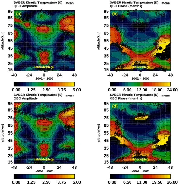
Fig. 2. Amplitude (left) and phase (right) for derived QBO temperature variations based on SABER data, plotted versus altitude (15 to
95 km) and latitude (48◦S to 48◦N). The top row (a) and (b) represents results for an assumed QBO period of 24 months obtained from year
days 2002001 to 2003365. For the bottom row (c) and (d) with 26-month QBO period, the results are obtained from data from year days 2002001 to 2004060.
For an assumed 24-month periodicity, we show in the top row of Fig. 2 the derived amplitudes (a) and phases (b) based on SABER temperature data from year day 2002001 to 2003365, plotted versus altitude (15 to 95 km) and lati-tude (48◦S to 48◦N). We cannot get reliable results pole-ward of about 48◦latitude since the measurements there are made only at alternate 60-day intervals. In the bottom row of Fig. 2, the corresponding results are presented for an as-sumed period of 26 months, based on data from year days 2002001 to 2004060. From this it can be seen that the basic features of the derived QBO signatures for the assumed peri-ods of 24 and 26 month are similar. The QBO amplitudes are prominent at equatorial latitudes (approaching 3.5◦K) and are mostly symmetric with respect to the Equator. But
signif-icant amplitudes also occur at mid-latitudes where they can approach 4◦K. With assumed periods of 28 and 29 months (not shown), the difference is mainly that the local amplitude maximum near 70 km is diminished relative to that for 24 and 26-month periodicities. The larger maxima between 25 and 40 km, and near 85 km, still remain essentially unchanged.
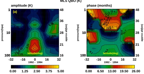
For comparison and analogous to Fig. 2, we present in Fig. 3 the derived temperature amplitudes and phases based on measurements from the MLS instrument on UARS. As-suming a period of 26 months, the QBO signature is derived from data between 100 and 1 hPa (about 16 and 48 km) for year days 1992001 to 1994060, about ten years before the SABER measurements (bottom row of Fig. 2). The MLS instrument does not produce data over as large an altitude
2136 F. T. Huang et al.: Stratospheric and mesospheric temperature variations 0.00 1.25 2.50 3.75 5.00 100 10 1 100 10 1 16 21 28 36 48 approx alt(km) -32 -16 0 16 32 100 10 1 1.00 1.00 1.00 1.25 1.25 1.50 1.50 1.75 1.75 2.00 2.00 2.25 2.25 pressure(hpa) latitude(deg) 1992 - 1994 MLS QBO (K) amplitude (K) (a) 0.00 6.50 13.00 19.50 26.00 100 10 1 100 10 1 16 21 28 36 48 approx alt(km) -32 -16 0 16 32 100 10 1 2.6 2.6 3.9 3.9 5.2 5.2 5.2 5.2 6.5 6.5 6.5 7.8 7.8 7.8 9.1 9.1 9.1 9.1 10.4 10.4 10.4 10.4 11.7 11.7 11.7 13.0 13.0 14.3 14.3 15.6 15.6 15.6 16.9 16.9 18.2 18.2 19.5 19.5 20.8 20.8 22.1 22.1 23.4 pressure(hpa) latitude(deg) 1992 - 1994 phase (months) (b)
Fig. 3. Analogous to Fig. 2 but for MLS (UARS) temperature measurements. Derived amplitude (a) and phase (b) variations for a 26-month QBO based on data from year days 1992001 to 1994060, plotted on altitude versus latitude coordinates commensurate with the limited coverage on UARS.
range as SABER does, and due to the UARS orbital char-acteristics, we do not get results pole-ward of 32◦ latitude. From Figs. 2 and 3, it appears that the QBO morphologies produced by the two instruments are similar, with the ampli-tude maxima occurring near the equator. The differences in phases between results based on SABER and on MLS data are understandable since the QBO periods are not constant. It can be seen that vertical wavelengths of about 30 km appear in both cases.
For comparison with other QBO results, we present with Fig. 4 the inferred SABER temperature variations themselves (rather and amplitudes and phases). In the left (a) and right (b) panels of the upper row, the temperature variations are shown for year days 2003075 (equinox) and 2002180 (sol-stice), which are obtained for an assumed 26-month QBO pe-riod from measurements for year days 2002001 to 2004060. The changes in phase with altitude and latitude below 45 km are qualitatively consistent with results from the United Kingdom Meteorological Office (UKMO) stratospheric as-similation (Randel et al., 1999, Baldwin et al., 2001), which are based on a combination of measurements and modeling. Our results show that the vertical phase changes continue at higher altitudes (UKMO results above 45 km were not pro-vided). There are also phase reversals with latitude above 45 km, although they are less extreme above about 70 km. The left plot (c) of the lower row is that portion of (a) be-tween 15 and 50 km and −32◦ and 32◦ latitude to better compare with the lower right plot (d) of Fig. 4, which is based on MLS data (year days 1992001 to 1994060) for year day 1992270, to correspond to equinox conditions. Note the small differences in plot limits between the two plots. MLS does not provide measurements over as large an altitude and
latitude range as does SABER. Considering that the QBO period is variable and phase comparisons are problematic, it is reasonable to conclude that the MLS and SABER mea-surements and the UKMO results for the stratosphere are in qualitative agreement.
Equatorial QBO
From the SABER and MLS results in Figs. 2 and 3 respec-tively, it is evident that the temperature QBO amplitudes in the stratosphere reach a maximum within about 10◦to 15◦ of the Equator. The peak values for this stratospheric QBO (SQBO) at altitudes from about 20 to 40 km approach 3.5◦K for SABER and MLS. For the mesospheric QBO (MQBO) at the Equator, the temperature peaks from SABER are smaller and sharper, i.e., about 3◦K near 70 km and 2◦K near 85 km. Our analysis with different QBO periods between 24 and 29 months shows that the peak near 85 km is more robust than that near 70 km.
The zonal winds of the QBO, which are confined to the tropics, are usually presented at latitudes near the Equator, plotted versus time and altitude. With the same format, we present with Fig. 5 in the left panel (a) the inferred QBO temperatures for a period of 24 months based on SABER data from year-days 2002001 to 2003365, and on the right the results for a 26-month oscillation based on data from 2002001 to 2004060. The variations are shown over two cy-cles to reveal the pattern more clearly. From this, it is evi-dent that in the stratosphere below 40 km, the QBO signature in the temperature propagates down with a velocity of about 1.3 km/month, which is in agreement with the observed zonal wind pattern. In the mesosphere, the propagation velocity is
-5.00 -2.50 0.00 2.50 5.00 15 25 35 45 55 65 75 85 95 -48 -24 0 24 48 15 25 35 45 55 65 75 85 95 -3.0 -2.5 -2.5 -2.0 -2.0 -2.0 -2.0 -1.5 -1.5 -1.5 -1.5 -1.0 -1.0 -1.0 -1.0 -1.0 1.0 1.0 1.0 1.01.52.0 altitude(km) latitude(deg) 2002 - 2004 QBO temperatures (K) SABER day 03075 (a) -5.00 -2.50 0.00 2.50 5.00 15 25 35 45 55 65 75 85 95 -48 -24 0 24 48 15 25 35 45 55 65 75 85 95 -1.0 1.0 1.0 1.0 1.0 1.0 1.5 1.5 1.5 1.5 1.5 2.0 2.0 2.5 altitude(km) latitude(deg) 2002 - 2004 SABER day 02180 (b) -5.00 -2.50 0.00 2.50 5.00 15 20 25 30 35 40 45 50 -32 -16 0 16 32 15 20 25 30 35 40 45 50 -2.0-1.5 -1.0 -1.0 -1.0 -1.0 -1.0 1.0 1.0 1.5 1.5 2.0 2.5 altitude(km) latitude(deg) 2002 - 2004 SABER day 03075 (c) -5.00 -2.50 0.00 2.50 5.00 100 10 1 100 10 1 16 21 28 36 48 approx alt(km) -32 -16 0 16 32 100 10 1 -2.0 -1.5 -1.0 -1.0 1.01.5 pressure(hpa) latitude(deg) 1992 - 1994 MLS day 93270 (d)
Fig. 4. Derived QBO temperature variations for selected days to illustrate the altitude-latitude morphology for 15 to 95 km and 48◦S to
48◦N. Top row based on SABER data for 26-month QBO: (a) at year day 2003075 for March equinox, and (b) at year day 2002180 for June
solstice. Bottom row for comparison between SABER and MLS results: (c) SABER results for 15 to 50 km and 32◦S to 32◦N from (a), and
(d) for MLS results at year day 1993270 based on data between 1992 and 1994. larger, and this is consistent with the larger eddy viscosity in
that region.
The literature on observed temperatures for the QBO in the stratosphere is relatively limited, and we are not aware of published QBO temperature measurements in the meso-sphere. For the middle and lower stratosphere, Dunker-ton and Delisi (1985b) analyzed 20 years of radiosonde data, while Pawson and Fiorino (1998), and Huesmann et al. (2001) discuss temperature results from the National Centers for Environmental Prediction (NCEP) and the Eu-ropean Centre for Medium-Range Weather Forecasts Re-analysis (ERA). Randel et al. (1999) presented results from the United Kingdom Meteorological Office (UKMO) anal-ysis. Remsberg et al. (2002) discuss the inter-annual
tem-perature variations based on data from the Halogen Occul-tation Experiment (HALOE) on UARS over a period of 9.5 years (October 1991 through April, 2001). In the altitude range between about 35 and 50 km, they detected varia-tions with periods from 688 to 800 days (about 23 to 27 months). Their amplitudes are typically around 1.0◦K, com-pared with the present SABER values that are closer to 3◦K, but the results are only given at 2 and 3 hPa (about 40 and 43 km). As discussed below, our results for the semiannual component agrees much better with those of Remsberg et al. (2002). With lidar measurements at Mauna Loa, Hawaii (19.5◦N), Leblanc and McDermid (2001) have observed QBO signatures in the stratospheric temperatures with am-plitudes approaching 5◦K, which are much larger than those
2138 F. T. Huang et al.: Stratospheric and mesospheric temperature variations -5.00 -2.50 0.00 2.50 5.00 15 25 35 45 55 65 75 85 95 15 25 35 45 55 65 75 85 95 -3.0 -3.0 -2.5 -2.5 -2.0 -2.0 -2.0 -2.0 -1.5 -1.5 -1.5 -1.5 -1.0 -1.0 -1.0 1.0 1.0 1.5 1.5 1.5 1.5 2.0 2.0 2.0 2.5 2.5 2.5 3.0 3.0 J A J O J A J O J A J O J A J O D Altitude(km) Data: 2002 - 2003 Equatorial QBO (K) Year day 2002001 - 2003365 (a) -5.00 -2.50 0.00 2.50 5.00 15 25 35 45 55 65 75 85 95 15 25 35 45 55 65 75 85 95 -2.5 -2.5 -2.0 -2.0 -1.5 -1.5 -1.5 -1.0 -1.0 -1.0 -1.0 -1.0 1.0 1.0 1.0 1.0 1.5 1.5 2.0 2.0 2.0 2.5 2.5 J A J O J A J O J A J O J A J O D Altitude(km) Data: 2002 - 2004 Year day 2002001 - 2004060 (b)
Fig. 5. Temperature variations at the Equator derived from SABER for QBO periods of 24 (a) and 26 (b) months, plotted versus altitude and month of year for two cycles. The results in (a) and (b) correspond to those presented in the top and bottom rows of Fig. 2 respectively.
-5.00 -2.50 0.00 2.50 5.00 -48 -24 0 24 48 -48 -24 0 24 48 -2.0 -1.0 -1.0 -1.0 -1.0 0.0 0.0 0.0 0.0 0.0 1.0 1.0 1.0 2.0
J FMAMJ J ASOND J FMAM J J ASOND
Latitude Data: 2002 - 2004 Derived QBO (K) (2002 - 2004) 25 km (a) -5.00 -2.50 0.00 2.50 5.00 -48 -24 0 24 48 -48 -24 0 24 48 -2.0 -2.0 -2.0 -1.0 -1.0 -1.0 -1.0 0.0 0.0 0.0 0.0 1.0 1.0 1.0 1.0 2.0 2.0
J FMAMJ J ASOND J FMAM J J ASOND
Latitude
Data: 2002 - 2004
40 km
(b)
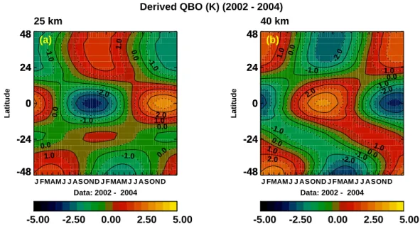
Fig. 6. For comparison with results from the United Kingdom Meteorological Office (UKMO) stratospheric assimilation (Randel et al., 1999), the QBO temperature variations based on SABER data at 25 km (a) and 40 km (b) are shown on latitude versus day coordinates.
inferred from SABER at this latitude. Contrary to our results for the mesosphere, Leblanc and McDermid (2001) also state that they have not detected any QBO temperature signatures from the lidar measurements above 60 km.
It is well established that the zonal winds for the QBO are confined to low latitudes and peak near the Equator (Bald-win et al., 2001). Consistent with our SABER tempera-ture results, a mesospheric QBO has been observed in the zonal winds with the HRDI instrument (Hays et al., 1993) on UARS (Burrage et al., 1996).
Mid-latitude QBO
It can be seen from Fig. 2 that the QBO temperature ampli-tudes generally recover from a minimum between 15◦ and 30◦ to reach again larger values at mid latitudes that are comparable to those near the Equator. For solstice in Fig. 4b, the temperature variations poleward of 20◦latitude reveal ev-ident asymmetries between the two hemispheres, which are not apparent in Fig. 4a for equinox. These asymmetries are apparent at least up to about 70 km. Although not shown,
the MLS results for solstice below about 50 km support the inferred asymmetry based on the SABER data. Since the global-scale meridional circulation is involved in generating the QBO temperature variations, and the meridional winds are directed across the equator from the summer to the win-ter hemisphere, it is reasonable to expect such asymmetries in the data. However, we have only two instances, and the observed asymmetries still could be coincidental.
Analogous to Fig. 5, we show with Fig. 6 the QBO tem-perature variations on latitude versus day of year coordinates based on 26-month SABER data at 25 km (a) and 40 km (b). As in the case for Fig. 4, the morphology is consistent with that from the UKMO stratospheric assimilation (Randel et al., 1999, Figs. 10, 11), where it is noted that the results at 25 and 40 km are mostly out of phase. The mid-latitude phase progression with altitude is markedly different from that at the Equator (Fig. 5), where the phase varies more gradu-ally with altitude. For example, near 20, 50 and 75 km (not shown) the phases at 40◦S to 48◦S undergo abrupt changes. We also have preliminary results (not shown) on temper-ature variations with longitude. Based on the SABER and MLS data, the results indicate that within about 20◦of the Equator, the QBO amplitudes vary little with longitude. At mid-latitudes, however, the apparent amplitude variations may approach 40 percent.
3.1.2 Semiannual Oscillations (SAO)
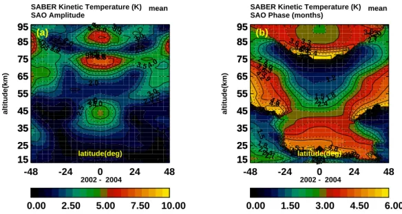
Analogous to Fig. 2, we present in Fig. 7 the amplitude (a) and phase (b) variations for the SAO temperatures obtained from the analysis of SABER data from years 2002, 2003, and 2004 merged together. The results are again shown on altitude (15 to 95 km) versus latitude (48◦S to 48◦N) coor-dinates. Corresponding results (not presented) based on data from individual years show that there are significant inter-annual variations in the amplitudes. As can be seen from Fig. 7, the temperature variations of the SAO are essentially symmetric with respect to the Equator. For the latitude range shown, the amplitudes tend to be largest close to the Equa-tor, especially at altitudes below about 55 km. Poleward of about 30◦ latitude, the amplitudes tend to level off and then increase with latitude, especially above 55 km.
Equatorial SAO
In the equatorial region (see Fig. 7, based on merged data from 2002, 2003, and 2004), our results for the stratospheric SAO (or SSAO) show an amplitude peak of about 5◦K at 45 km altitude. At higher altitudes, it is evident from Fig. 7 that there are two separate amplitude peaks approaching 7◦K, one near 75 km and the second one near 90 km. The inter-annual variations of the SAO, mentioned above, show that the inferred amplitudes are largest in 2002 compared to those of 2003 and 2004. An example is given in Fig. 8, in which the estimated semiannual temperatures are plotted at
the Equator on altitude versus day of year coordinates. In the left panel (a), we show the analysis result for the combined 2002, 2003, and 2004 data, while the right plot (b) is based on data from 2002 only.
Remsberg et al. (2002) derived the amplitude and phase variations for the temperature of the SAO based on HALOE measurements on UARS, covering over 9.5 years (October, 1991 through April, 2001). The results are presented from 10 to 0.01 hPa (about 32 to 80 km) and from 40◦S to 40◦N. The contour plots (from Fig. 4 of their paper, not shown) can be compared directly with our Fig. 7, and show that the SAO amplitude and phase variations for the measured tem-peratures on UARS (HALOE) and TIMED (SABER) are in qualitative agreement. At the Equator, both data sets pro-duce peak amplitudes of about 6◦K centered between 70 and 75 km, but the apparent peak of about 2◦K in the amplitudes based on HALOE data near 40 km is only about half as large as the one inferred from SABER. Remsberg et al. (2002) do not provide results above 80 km, and therefore cannot verify the amplitude peak we find near 90 km.
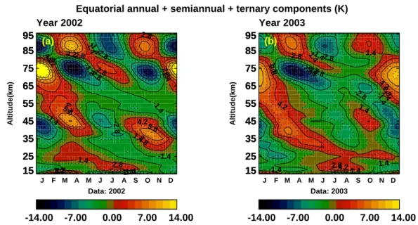
For our SAO results near 90 km however, we believe that the analysis by Garcia et al. (1997) does provide some confirmation. They analyzed the temperature data from the Solar Mesosphere Explorer (SME) satellite (measured by the ultraviolet spectrometer (UVS) from 40 to 92 km, years 1983 to 1986) and from rocketsondes at Kwajalein (8.7◦N, 167.7◦W) and Ascension (7.6◦S, 14.4◦W) islands. The rocketsonde measurements covered altitudes from the ground to 63 km, years 1969 to 1987. The results by Gar-cia et al. (not shown here) were presented for the combined annual, semiannual, and ternary harmonics, and they were plotted on altitude versus latitude coordinates. For compar-ison, we present with Fig. 9 the corresponding results based on SABER data at the Equator, which also contain the com-bined annual, semiannual and ternary components. The left panel (a) is based on data from year 2002 and the right plot (b) is based on data from year 2003 to show inter-annual vari-ations.
In Fig. 9, the altitudes from about 15 to 60 km cover the range for the temperature observations by Garcia et al. (1997) at Kwajalein and Ascension islands. Our SABER results agree morphologically with those published by Garcia et al. But their temperature variations are smaller than ours, with lows and highs being generally between −2 and 4◦K, re-spectively. As they point out, the sounding rocket data were averaged into months and otherwise smoothed to study the seasonal cycles. Moreover, the rocketsonde data were taken primarily during the early afternoon hours, so that they were biased by thermal tides. Both the rocketsonde and our re-sults show that the annual cycle starts to dominate near the tropopause, although the transition from the semi-annual cy-cle occurs in the SABER data at altitudes 2 or 3 km higher. For the Garcia et al. results based on SME data at the Equa-tor, the inferred SAO temperature variations cover the alti-tude range from 40 to 92 km. Our derived SAO temperatures
2140 F. T. Huang et al.: Stratospheric and mesospheric temperature variations 0.00 2.50 5.00 7.50 10.00 15 25 35 45 55 65 75 85 95 -48 -24 0 24 48 15 25 35 45 55 65 75 85 95 1.0 1.0 1.0 1.5 1.5 2.0 2.0 2.0 2.0 2.5 2.5 2.5 2.5 3.0 3.0 3.0 3.0 3.0 3.5 3.5 3.5 3.5 4.0 4.0 4.0 4.0 4.5 4.5 5.0 5.0 5.56.06.5 altitude(km) latitude(deg) 2002 - 2004 SABER Kinetic Temperature (K)
SAO Amplitude mean
(a) 0.00 1.50 3.00 4.50 6.00 15 25 35 45 55 65 75 85 95 -48 -24 0 24 48 15 25 35 45 55 65 75 85 95 1.2 1.2 1.2 1.5 1.5 1.5 1.5 1.8 1.8 1.8 1.8 1.8 2.1 2.1 2.1 2.1 2.4 2.4 2.4 2.4 2.7 2.7 2.7 2.7 3.0 3.0 3.0 3.0 3.3 3.3 3.3 3.3 3.6 3.6 3.6 3.6 3.6 3.9 3.9 3.9 3.9 4.2 4.2 4.2 4.2 4.5 4.5 4.5 4.5 4.8 4.8 4.8 4.8 5.1 5.1 5.15.4 altitude(km) latitude(deg) 2002 - 2004 SABER Kinetic Temperature (K) SAO Phase (months) mean
(b)
Fig. 7. Amplitudes (left) and phases (right) for derived SAO temperature variations based on SABER data, plotted versus altitude (15 to
95 km) and latitude (48◦S to 48◦N). The data from years 2002, 2003, and 2004 were merged together to derive the SAO.
-12.00 -6.00 0.00 6.00 12.00 15 25 35 45 55 65 75 85 95 15 25 35 45 55 65 75 85 95 -2.4 -2.4 -2.4 -1.2 -1.2 -1.2 1.2 1.2 2.4 1.2 2.4 2.4 2.4 2.4 3.6 J F M A M J J A S O N D Altitude(km) Data: 2002 - 2004
Equatorial semiannual component (K) Year 2002 - 2004 combined (a) -12.00 -6.00 0.00 6.00 12.00 15 25 35 45 55 65 75 85 95 15 25 35 45 55 65 75 85 95 -3.6 -3.6 -2.4 -2.4 -2.4 -2.4 -1.2 -1.2 -1.2 -1.2 1.2 1.2 1.2 1.2 1.2 2.4 2.4 2.4 2.4 2.4 2.4 3.6 3.6 3.6 3.6 3.6 4.8 4.8 4.8 J F M A M J J A S O N D Altitude(km) Data: 2002 Year 2002 (b)
Fig. 8. SABER derived temperature variations for the SAO are shown at the Equator plotted on altitude versus day coordinates. (a) Corresponds to Fig. 7 for years 2002 to 2004 merged together, and (b) for comparison from year 2002 to illustrate the inter-annual variability of the SAO.
are more consistent with the rocketsonde results than with the SME data, although there is general agreement that the semiannual component tends to dominate. Between 60 and 80 km, the SME values are generally between −4◦K and 4◦K, and are smaller than our highs and lows, as can be seen from Fig. 9a. From our figure, it can also be seen that rel-atively rapid phase changes with altitude occur near 80 km, and this feature is also evident in the SME results. Unlike the situation at lower altitudes, the SME temperature amplitudes
above 85 km can approach 16◦K and are significantly larger than our highs and lows of about ±8◦K. Otherwise, the am-plitudes aside, our results track the SME data very closely in time. Garcia et al. (1997) question the accuracy of the large SAO values and the morphology based on SME data. They note that above 85 km, the SME results are not consis-tent with (a) the corresponding vertical shears of the zonal winds from the High Resolution Doppler Imager (HRDI) on the Upper Atmosphere Research Satellite (UARS) satellite,
-14.00 -7.00 0.00 7.00 14.00 15 25 35 45 55 65 75 85 95 15 25 35 45 55 65 75 85 95 -4.2 -2.8 -2.8 -2.8 -2.8 -1.4 -1.4 -1.4 -1.4 -1.4 1.4 1.4 1.4 1.4 1.4 1.4 2.8 2.8 2.8 2.8 2.8 2.8 2.8 2.8 4.2 4.2 4.2 4.2 4.2 5.6 5.6 J F M A M J J A S O N D Altitude(km) Data: 2002
Equatorial annual + semiannual + ternary components (K) Year 2002 (a) -14.00 -7.00 0.00 7.00 14.00 15 25 35 45 55 65 75 85 95 15 25 35 45 55 65 75 85 95 -7.0-5.6-4.2 -2.8 -2.8 -2.8 -1.4 -1.4 -1.4 -1.4 1.4 1.4 1.4 1.4 1.4 1.4 2.8 2.8 2.8 2.8 4.2 4.2 4.2 J F M A M J J A S O N D Altitude(km) Data: 2003 Year 2003 (b)
Fig. 9. Similar to Fig. 8 but showing the derived combined annual, semiannual, and ternary components at the Equator based on SABER measurements. (a) Based on data from year 2002; (b) for year 2003 to illustrate inter-annual variability.
(b) with the results from sounding rockets at Ascension and Kwajalein Islands, and (c) with the MF radar measurements at Christmas Island (2◦N, 157◦W). They also noted that the diurnal tides in the SME data were not accounted for, and the zonal averages could be biased because the longitude cover-age was not uniform. Notwithstanding these difficulties, the two peaks in the SAO temperature amplitude derived from the SABER measurements in the mesosphere are qualita-tively consistent with the results from SME near 90 km. In contrast to SME, the TIMED mission samples all local times, and the algorithm we use effectively removes the tidal com-ponent from the SABER data. As shown in the next section, the amplitudes for the diurnal tide can approach 20◦K.
Fleming et al. (1990, COSPAR International Reference Atmosphere) report peak amplitudes of about 4◦K for the inferred SAO temperatures near 40 km and 80 km, which is comparable to ours and larger than that of Remsberg et al. (2002) in the stratosphere, but is smaller than ours and that of Remsberg et al. in the mesosphere. They do not show an amplitude peak near 90 km, as we do. The phase variations are similar to ours, with some differences in de-tails. The SAO temperature amplitudes derived by Shepherd et al. (2004) from measurements by the Wind Imaging Inter-ferometer (WINDII) on UARS at 75 km agree to about 10 to 15 percent, while the phases generally differ by less than one month.
In addition to the effects from tidal variations and other problems mentioned earlier, there are other possible reasons for the differences between our results and those of others. The data with which we compare often cover a longer time span, and our zonal means are not averaged in time such as in monthly bins. In addition, other results generally use one set
of amplitudes and phases to represent the entire multi-year data sets.
For the zonal winds of the SAO at the Equator, peak am-plitudes have been reported in the stratosphere near 45 km and in the mesosphere near 80 km (Hirota, 1978; Balwin et al., 2001).
Mid-latitude SAO
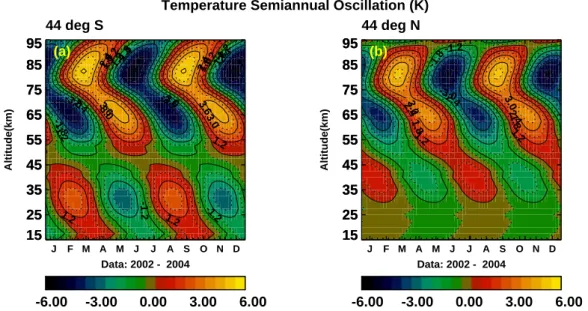
From Fig. 7 it is apparent that the derived SAO tempera-ture amplitudes, between 48◦S and 48◦N, tend to peak at the Equator. Above about 55 km, however, the amplitudes increase again pole-ward of about 30◦ latitude. At 48◦ in both hemispheres, the amplitudes reach several◦K near 35, 60, and 80 km, and one might expect that they would con-tinue to increase further at higher latitudes. Analogous to Fig. 8, we show in Fig. 10 the estimated semiannual temper-ature amplitudes (◦K) on altitude versus day coordinates at 44◦S (a) and 44◦N (b), based on data from years 2002–2004 merged into one 365-day period. The existence of substan-tial temperature amplitudes at mid-latitudes is qualitatively consistent with results based on lidar measurements (Leblanc et al., 1998), from stations at 44◦N in France (Observatoire de Haute Province (OHP) and Centre d’Essais des Landes (CEL)) and at 40.6◦(Colorado State University (CSU)). The results of Remsberg et al. (2002) do not extend past 40◦, but they indicate also that the amplitudes recover at mid-latitudes though with smaller magnitudes than those reported here.
2142 F. T. Huang et al.: Stratospheric and mesospheric temperature variations -6.00 -3.00 0.00 3.00 6.00 15 25 35 45 55 65 75 85 95 15 25 35 45 55 65 75 85 95 -3.6 -3.0-2.4 -3.0 -2.4 -2.4 -1.8 -1.8 -1.8 -1.2 -1.2 -1.2 -1.2 -1.2 1.2 1.2 1.2 1.2 1.2 1.8 1.8 2.4 2.4 3.0 3.0 3.6 3.6 J F M A M J J A S O N D Altitude(km) Data: 2002 - 2004
Temperature Semiannual Oscillation (K) 44 deg S (a) -6.00 -3.00 0.00 3.00 6.00 15 25 35 45 55 65 75 85 95 15 25 35 45 55 65 75 85 95 -3.0-2.4 -1.8 -1.2 1.2 1.2 1.8 1.8 2.4 2.4 3.0 3.0 J F M A M J J A S O N D Altitude(km) Data: 2002 - 2004 44 deg N (b)
Fig. 10. Analogous to Fig. 8 but showing the derived temperature variations for the SAO at 44◦S (a) and 44◦N (b) based on SABER data from years 2002 to 2004 merged together.
3.2 Diurnal tides
We recall that in their discussion of the SAO, Garcia et al. (1997) emphasized that the sun-synchronous SME and the rocketsonde measurements did not provide information on the diurnal variations, and they questioned therefore the accuracy of their results. As mentioned above, over a period of 60 (SABER) and 36 (MLS) days, the data are sampled over the range of local times, and our algorithm accounts for the variations of the tides. Although the focus of this paper is not on thermal tides, for completeness we present some of the results that bear on their inter-annual variations.
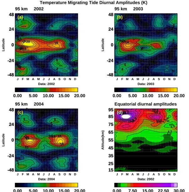
In Fig. 11, we present the derived amplitudes for the diur-nal migrating tide based on SABER temperatures at 75 km. The panels (a), (b), (c) show the results for the years 2002, 2003, 2004, respectively, plotted on latitude versus day of year coordinates, and the lower right panel (d) shows the diurnal migrating tide amplitudes for year day 2002080 on altitude-latitude coordinates. Corresponding to Fig. 11, the tidal results for 95 km are shown in Fig. 12. The lower right panel (d) of Fig. 12 shows the temperature migrating tide diurnal amplitudes for year 2002 at the Equator on altitude versus day of year coordinates. In panels (d) of Figs. 11 and 12, near the maximum values, we have allowed the colors to saturate so that the colors near minimum values can be dis-cerned more easily. Characteristic for the propagating diur-nal tide, the temperature amplitude peaks at the equator and near equinox. In the context of the present paper, the tide also varies significantly from year to year, presumably under the influence of the QBO. Such inter-annual variations of the diurnal tide have also been reported by Burrage et al. (1996) based on wind measurements with the HRDI instrument on UARS (Hays et al., 1993).
4 Numerical Spectral Model (NSM) results
For comparison with the above observations, we present here the numerical results from a study with the Numerical Spec-tral Model (NSM) in which the inter-annual variations of the diurnal tide were generated by the wave-driven Quasi-biennial Oscillation (Mayr and Mengel, 2005, referred to as MM). No attempt was made in this model run to tune the NSM to reproduce the measurements. The model compari-son is of interest since it documents where we presently stand with the NSM and thereby illustrates some of our difficulties in simulating the observed equatorial oscillations (i.e., QBO and SAO).
In the following, we briefly describe the NSM and the spe-cific model run in MM from which the numerical results are taken. We then present the computed zonal mean tempera-ture variations that characterize the QBO and SAO. For the diurnal tide, we refer to the inter-annual variations of the tem-perature amplitude that are shown in Fig. 2e of MM.
The MM version of the NSM is integrated from the Earth’s surface into the lower thermosphere and is driven for the zonal mean (m=0) by ultraviolet radiation in the mesosphere, and in the stratosphere the heating is taken from Strobel (1978), and by extreme ultraviolet radiation absorbed in the thermosphere. For m=0, tropospheric heating is ap-plied to reproduce qualitatively the observed zonal jets near the tropopause and the accompanying latitudinal tempera-ture variations. The migrating tides are driven by the ex-citation sources in the troposphere and stratosphere (Forbes and Garret, 1978), and non-linear interactions between mi-grating tides and planetary waves generate the non-mimi-grating tides. Since the model does not have topography, the plane-tary waves are generated solely by instabilities. The radiative
0.00 5.00 10.00 15.00 20.00 -48 -24 0 24 48 -48 -24 0 24 48 2 2 2 2 2 2 2 4 4 4 4 4 4 6 6 6 8 8 10 12 J F M A M J J A S O N D Latitude Data: 2002
Temperature Migrating Tide Diurnal Amplitudes (K) 75 km 2002 (a) 0.00 5.00 10.00 15.00 20.00 -48 -24 0 24 48 -48 -24 0 24 48 2 2 2 2 2 2 2 2 4 4 6 8 8 J F M A M J J A S O N D Latitude Data: 2003 75 km 2003 (b) 0.00 5.00 10.00 15.00 20.00 -48 -24 0 24 48 -48 -24 0 24 48 2 2 2 2 2 2 2 4 4 4 4 4 6 6 6 8 8 10 10 J F M A M J J A S O N D Latitude Data: 2004 75 km 2004 (c) 0.00 7.50 15.00 22.50 30.00 15 25 35 45 55 65 75 85 95 -48 -24 0 24 48 15 25 35 45 55 65 75 85 95 1.5 1.5 1.5 1.5 3.0 3.0 4.5 4.5 4.5 4.5 6.0 6.0 6.0 7.5 7.5 7.5 9.0 10.5 12.0 13.5 altitude(km) latitude(deg) 2002 Day 2002080 (d)
Fig. 11. For the migrating diurnal tide, the temperature amplitudes are presented at 75 km, which are derived from the SABER data jointly
with the earlier discussed zonal-mean components. Plotted versus latitude (48◦S to 48◦N) and month of year for 2002 (a), 2003 (b), and
2004 (c) to illustrate the inter-annual variability of the tide. Lower right (d): Diurnal tidal amplitudes for day 2002080 on altitude versus day coordinates.
loss is described in terms of Newtonian cooling adopted from Zhu (1989), which is modified to keep the radiative relax-ation rate constant below 20 km.
An integral part of the NSM is that it incorporates the Doppler Spread Parameterization (DSP) for small-scale gravity waves (GWs) developed by Hines (1997a, b). The DSP deals with a spectrum of waves that interact with each other to produce Doppler spreading, which affects the GW interactions with the flow. To account for the enhanced wave activity in the tropics due to convection, the GW source in MM is assumed to peak at the equator – and this contributes to generate the stronger QBO zonal wind amplitudes in the stratosphere that are fairly realistic in this model run. Since
there is very little observational guidance, the GW parame-ters were chosen simply from the middle of the range rec-ommended for the DSP. The non-linear DSP is implemented with Newtonian iteration, and convergence is enforced by ad-justing the time integration step that is typically 5 min. With the upper boundary at about 130 km, an integration step of about 0.5 km is chosen to resolve the GW interactions with the flow, but the NSM is truncated at the zonal and merid-ional wave-numbers m=4 and n=12, respectively.
4.1 QBO model
The QBO generated by the NSM in MM has a period that varies between about 22 and 30 months, which qualitatively
2144 F. T. Huang et al.: Stratospheric and mesospheric temperature variations 0.00 5.00 10.00 15.00 20.00 -48 -24 0 24 48 -48 -24 0 24 48 2 2 2 2 2 2 2 4 4 4 4 4 4 4 4 6 6 6 6 6 8 8 8 8 10 10 12 1416 16 1820 J F M A M J J A S O N D Latitude Data: 2002
Temperature Migrating Tide Diurnal Amplitudes (K) 95 km 2002 (a) 0.00 5.00 10.00 15.00 20.00 -48 -24 0 24 48 -48 -24 0 24 48 2 2 2 2 2 2 4 4 4 4 4 4 4 6 6 6 6 6 6 8 8 8 8 101214 J F M A M J J A S O N D Latitude Data: 2003 95 km 2003 (b) 0.00 5.00 10.00 15.00 20.00 -48 -24 0 24 48 -48 -24 0 24 48 2 2 2 2 2 2 2 4 4 4 4 4 4 4 4 6 6 6 6 6 8 8 8 8 10 10 1214 12 14 16 16 J F M A M J J A S O N D Latitude Data: 2004 95 km 2004 (c) 0.00 7.50 15.00 22.50 30.00 15 25 35 45 55 65 75 85 95 15 25 35 45 55 65 75 85 95 1.5 1.5 1.5 1.5 1.5 1.5 3.04.5 4.5 6.0 7.5 9.0 10.5 12.0 12.0 13.5 15.0 16.5 18.019.522.521.0 J F M A M J J A S O N D Altitude(km) Data: 2002
Equatorial diurnal amplitudes
(d)
Fig. 12. Upper row and lower left (a), (b), (c): Similar to Figu. 11 but for derived year-to-year variations of the migrating diurnal tide at 95 km, for years 2002, 2003, 2004. Lower right (d): Migrating diurnal tidal amplitudes for 2002 at the Equator on altitude versus day coordinates.
mimics the variability that is observed. To get modeled QBO results that are fairly stable for at least 2 cycles, we chose the time segment after year 17 where the period is close to 24 months. For that period, we present in Fig. 13 the amplitude and phase variations of the computed QBO temperatures. This shows that the temperature amplitudes in the strato-sphere below 60 km approach values close to 2◦K, which are smaller than those observed (exceeding 3◦K) below 40 km (see Fig. 2). In qualitative agreement with the SABER mea-surements, the model generates a mesospheric temperature QBO above 60 km, but the amplitude there is only 1◦K com-pared to the measured values of about 3◦K. In contrast to the modeled zonal winds, the temperature variations of the QBO are not confined to the equatorial region. This is in qualita-tive agreement with the measurements, including the phase
reversals at latitudes away from the equator. Hemispherical asymmetries also appear in both the model results and the observations. However, the temperature amplitudes outside the equatorial region tend to occur at lower latitudes in the model results.
For comparison with the observed QBO temperature vari-ations at the Equator (see Fig. 5), we present in Fig. 14 the corresponding model results for 4◦latitude (Gaussian point). This shows the downward phase progression that character-izes the QBO zonal winds at the Equator. In qualitative agreement with the observations, the downward phase ve-locity increases from the stratosphere into the mesosphere. However, that phase speed increases roughly from about 1.3 to 3 km/month in the observations and from about 1 to 1.8 km/month in the model results.