HAL Id: hal-01286537
https://hal-centralesupelec.archives-ouvertes.fr/hal-01286537
Submitted on 11 Mar 2016
HAL is a multi-disciplinary open access
archive for the deposit and dissemination of
sci-entific research documents, whether they are
pub-lished or not. The documents may come from
teaching and research institutions in France or
abroad, or from public or private research centers.
L’archive ouverte pluridisciplinaire HAL, est
destinée au dépôt et à la diffusion de documents
scientifiques de niveau recherche, publiés ou non,
émanant des établissements d’enseignement et de
recherche français ou étrangers, des laboratoires
publics ou privés.
Layered Electric-Current Approximations of Cylindrical
Sources
Andrea Cozza, F Monsef
To cite this version:
Andrea Cozza, F Monsef. Layered Electric-Current Approximations of Cylindrical Sources. Wave
Motion, Elsevier, 2016, 64, pp.34-51. �10.1016/j.wavemoti.2016.03.002�. �hal-01286537�
Layered Electric-Current Approximations of Cylindrical Sources
A. Cozzaa, F. Monsefa aPhysique et Ingénierie de l’Électromagnétisme
Group of Electrical Engineering of Paris (GeePs), CNRS UMR 8507, CentraleSupelec - Univ Paris-Sud - UPMC 11 rue Joliot-Curie, Plateau de Moulon, 91192 Gif-sur-Yvette, France.
Contact : [email protected]
Abstract
Formulations of the equivalence theorem only involving electric currents either imply non-null inner fields, or the inclusion of a bulk perfect magnetic conductor. The possibility of maintaining a homogeneous background medium across the equivalent-current surface and null inner fields without recurring to magnetic currents is here investigated for the case of cylindrical sources. The proposed procedure keeps using the definition of equivalent electric currents as found in A. Love’s theorem, introducing further layers of auxiliary electric currents to mimic the role of the missing magnetic ones. Optimal scalar coefficients applied as weights on each layer current are found, so to minimize the mean quadratic error in the fields radiated outside the auxiliary shell region, while at the same time minimizing internal radiation. The procedure is inherently well-conditioned, thanks to the reduction in the number of degrees of freedom involved, equal to the number of layers, as forced by a regression approach. A thorough numerical analysis is presented, where residual errors are found to be in the range of a few percent points.
Keywords: Cylindrical sources, equivalent currents, modal theory, antennas.
1. Introduction
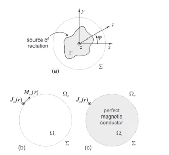
Equivalence theorems are a workhorse of antenna theory, widely applied in order to simplify the analysis and the com-putation of fields generated by a source of radiation. Initially derived by Love and MacDonald more than a century ago [1, 2], they can be flexibly declined into versions that can suite a large number of practical configurations [3, 4, 5]. Independently from the specific version, they all share the same basic idea, illustrated in Fig. 1: given an original sourceΓ, identify a spa-tial distribution of equivalent currents over a closed surfaceΣ containingΓ, such that these currents generate a perfect repro-duction of the field distribution expected forΓoverΩe, outside
Σ. Analogue versions exist for a sourceΓoutsideΣ, a case not treated in this paper .
Referring to the nowadays standard formulation due to Schelkunoff [6], equivalent electric, Jeq(r ), and magnetic, Meq(r ), currents are required, if the equivalent problem in
Fig. 1(b) is to work in a homogeneous medium across the sur-faceΣ. In this case, it can be shown that [1]
Jeq(r ) =δ(r − rΣ) ˆn(rΣ) × H (r ) (1a) Meq(r ) =δ(r − rΣ)E (r ) × ˆn(rΣ), (1b)
whereE(r ) andH(r )are, respectively, the electric and mag-netic field generated by the original source at the position r;
δ(·) is Dirac’s delta distribution, here used in order to repre-sent a singular current sheet limited toΣ;nˆ(rΣ)is the outward
unit vector normal toΣ, at the positionrΣ. A time convention exp(jωt )is assumed, but only phasors are shown. All quantities are frequency dependent, but the pulsationωis dropped for the sake of brevity. M r eq( ) S (a) Jeq( )r r ^ source of radiation x y z j (b) S Wi We (c) S Wi We Jeq( )r perfect magnetic conductor G
Figure 1: Original source of radiation (a) and two equivalent-current configu-rations, with a homogeneous background medium using electric and magnetic currents (b) and with only electric currents with the internal region filled by a perfect magnetic conductor (c).
In case the fields radiated by a source were obtained through experiments, both electric and magnetic fields would need to be accessed; in practice, only probes sensitive to one kind of field could be available. Equivalent electric currents suffice ifΩi is
filled with an ideal perfect magnetic conductor (see Fig. 1(c)), as described in [6], ensuring a perfect field reproduction over Ωe. Unfortunately, reproducing this kind of scenario in a
nu-merical model, a bulk material inΩi would behave as a
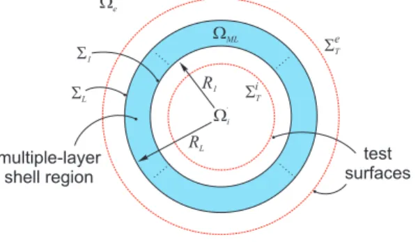
ST ST S1 SL test surfaces multiple-layer shell region We WML e i ’ ’ Wi R1 RL
Figure 2: The paradigm considered in this paper: Lmultiple-layer auxiliary electric-current distributions are found in a shell shown in shade, each occupy-ing a surfaceΣi. Internal and external test surfacesΣiTandΣeT, as introduced in sec. 4, are used for the optimization of the layer weights. The new inner and outer regions are referred to as primed quantities, to differentiate them from those defined in standard equivalent-theorem formulations (see Fig. 1).
terer in case waves impinged onto it. Formulations using only electric currents while keeping a homogeneous medium across Σwould be required in this case, as discussed in [7].
Solutions for this problem can be defined, as shown in [4, 8, 9, 10, 11], but imply non-null fields inΩi. This can be
a problem since inward radiation inevitably leads to outward waves after propagating throughΩi. In this paper we are
in-terested in equivalent currents that radiate only outside Σ, as a continuation of the fields radiated by the original sourceΓ; therefore, null fields are required inΩi.
To this end, magnetic equivalent currents could be converted into an additional electric contributionJM(r ) = ∇×Meq(r )/jωµ
[12]. But in case of an experimental characterization of the original source, this operation is ill-posed, since it involves estimating derivatives from measurements. Critically, normal derivatives would require sampling fields at different distances from the original source. Moreover, this further electric-current contribution now involves spatial derivatives of a Dirac distri-bution, which does not correspond to a double-sheet of currents. In order to overcome these difficulties, this paper suggests using multiple layers of electric currents, defining a shell re-gionΩMLas shown in Fig. 2. The rationale is to make the fields
radiated by the different layers of currents interfere, in such a way as to emulate the interplay between fields radiated by elec-tric and magnetic currents in Love’s theorem.
Our proposal is not to set up an inverse problem where the equivalent current distributions over each layer would act as unknowns, since this kind of approach is often ill-conditioned, particularly in the case of measured data. We rather attempt ex-tending the use of distributions defined as in (1a) over at least two surfaces, by defining optimal scalar coefficients acting as weights on each of these current distributions. As it will be shown in the rest of the paper, the proposed method, though effective, does not allow a perfect equivalence, hence our refer-ring to these currents as auxiliary rather than equivalent.
2. Scalar representation of the problem
In the following we will consider the case of original sources described by means of electric-current distributions confined within a shell region of spaceΩML(Fig. 2). For ease of
deriva-tion, a cylindrical geometry will be assumed, with translation invariance to axial displacements.
Dealing with cylindrical sources, it is convenient to proceed by separating the original currents modelling the source over the regionΓ(Fig. 1) into axial and transversal components
Js(r ) = JËs(r ) + J⊥s(r ) = ˆz JsË(r ) + ˆϕJ⊥s(r ), (2) where bold variables represent vector quantities while hatted ones are unit vectors. In order to simplify our derivation, we introduce magnetic currents [12, section 7.12]
MËs(r ) = ˆz MsË(r ) = −
1 jωǫ∇ × J
⊥
s(r ). (3)
In the following, instead of the original current distribution (2) we will consider a source described by axial currentsJËs(r )and MËs(r ).
Maxwell’s equations for cylindrical configurations can be ex-pressed as [12, section 14.1] ¡∇2+ ω2ǫµ¢2 EË(r ) = −jωµJËs(r ) − ∇ · (ˆz × M ⊥ s(r )) (4) ¡∇2+ ω2ǫµ¢2 HË(r ) = −jωǫMsË(r ) − ∇ · (ˆz × J ⊥ s(r )), (5)
hence describing the source through only axial electric and magnetic currents yields scalar decoupled equations
¡∇2+
ω2ǫµ¢2EË(r ) = −jωµJËs(r ) (6)
¡∇2+
ω2ǫµ¢2
HË(r ) = −jωǫMsË(r ), (7)
corresponding to a TM (transverse-magnetic) and TE (transverse-electric) problem, respectively. Hence, (6) is solved by EË(r ) =ωµ 4 Z Γ dr′H0(k0kr − r′k)JsË(r′), (8)
whereH0(·) is Hankel’s function of zero-th order of the first
kind (i.e., for an outgoing wave). Equation (8) is also a solution to (7), by substituting electric-field related quantities with mag-netic ones, as according to the duality principle; for this reason, the rest of the paper will only focus on the case of axial elec-tric sources. Solutions found for this problem can be readily applied to the case of azimuthal electric sources thanks to (3).
3. Fields radiated by a single layer of electric currents We first seek a modal expansion of the electromagnetic field radiated by the original source inΓ, by applying the addition theorem to (8), here recalled for the sake of completeness, for the special case of the outgoing Hankel function of the zeroth order H0(kokr − r′k) = ∞ X m=−∞ Jm(kor′)Hm(kor )ejm(ϕ−ϕ ′) r′<r ∞ X m=−∞ Hm(kor′)Jm(kor )ejm(ϕ−ϕ ′ ) r′> r (9)
whereJm(·)andHm(·)are Bessel’s and Hankel’s functions of themth order of the first kind. From (8) and (9) we straightfor-wardly obtain EË(r ) =ωµ 4 ∞ X m=−∞ γmψhm(r ) r∈ Ωe, (10)
having introduced a shorthand representation of cylindrical modes
ψhm(r ) = Hm(kor )ejmϕ (11a) ψmj (r ) = Jm(kor )ejmϕ (11b)
and the associated modal weights
γm= Z Γ dr′ hψmj (r′) i∗ JeË(r′), (12)
with∗the complex conjugate.
The magnetic field can also be represented in a similar man-ner; making use of the electric-field curl equation,
H⊥(r ) = j 4 ∞ X m=−∞ γm∇ ×hˆzψhm(r ) i = = ∞ X m=−∞ γm · ˆ rjm r −ϕˆ∂r ¸ ψhm(r ), (13)
where∂r is the first-order derivative taken with respect to the radial distancer.
In order to understand what is the effect of removing equiv-alent magnetic currents in a free-space configuration, we con-sider a cylindrical surfaceΣ, of radiusR, over which
JeqË(r ) = −δ(r − R) ∞ X m=−∞ γmejmϕ∂rHm(kor ), (14) as given by (1) and (13).
The electric field generated by these currents can be com-puted by applying (8) to the current distribution (14). The ap-plication of the addition theorem (9) yields
ˆ EË(r ) =ωµ 4 ∞ X m=−∞ γm ( ηem(R)ψhm(r ) r∈ Ωe ηim(R)ψ j m(r ) r∈ Ωi (15) with
ηem(R) = −jπR Jm(koR)∂RHm(koR) (16a) ηim(R) = −jπRHm(koR)∂RHm(koR). (16b)
The corresponding magnetic field is
ˆ H⊥(r ) =j 4 ∞ X m=−∞ γm · ˆ rjm r −ϕˆ∂r ¸ ( ηem(R)ψhm(r ) r∈ Ωe ηim(R)ψ j m(r ) r∈ Ωi . (17)
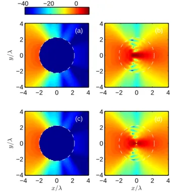
Fig. 3 shows an example of the electric and magnetic field distributions for the ideal case expected for the equivalence the-orem, and those observed in the case where only equivalent
y / λ −4 −2 0 2 4 −4 −2 0 2 4 −4 −2 0 2 4 −4 −2 0 2 4 x/λ y / λ −4 −2 0 2 4 −4 −2 0 2 4 x/λ −4 −2 0 2 4 −4 −2 0 2 4 −40 −20 0 (a) (b) (c) (d)
Figure 3: An example of electric (b) and magnetic (d) fields radiated by a single layer of equivalent electric currents, here represented by the dashed circle. Ref-erence field distributions expected for the case of electric and magnetic equiva-lent currents are shown on the left column, respectively for the electric (a) and magnetic (c) field. Corresponding field distributions generated by the electric currents alone are given on the right column. Data represent the amplitude of the fields measured in dB, normalized to the peak amplitude observed for the reference distribution.
electric currents are present, i.e., a partial application of the equivalence theorem. These results refer to the test-case de-scribed in section 8, dealing with a directive linear source four wavelengths long. This source has a directive leftward radia-tion.
In the case of partial application of the equivalence theorem, the leftward radiation is well reproduced, whereas a spurious rightward radiation appears. This last is due to the fact that equivalent electric currents that are at the origin of the leftward radiation do also radiate towards the inner regionΩi; this
in-ward radiation would be counterbalanced by equivalent mag-netic currents in the equivalence-theorem free-space formula-tion. Left alone, the inward contribution may focus inside the inner regionΩi and subsequently diverge rightwards, causing
the spurious radiation that did not appear in the original config-uration. Hence the need for an alternative mechanism of control of the inward radiation.
4. Multiple-layer auxiliary currents
Reproducing the results of Love’s formulation would require, apart for a common constant factor, to ensure that ηe
m(R) =
1, ∀m andηim(R) = 0, ∀m. In other words, theηi,em(R)
co-efficients act as distortions, in the modal expansion of the field distribution generated by the original electric currentsJËe(r ), by 3
passing, e.g., for the region external to Σ, from modal coeffi-cients{γm}to{γmηe
m(R)}.
Our proposal is to introduce multiple layers of auxiliary cur-rent distributions, defined as in Fig. 2 overLconcentric cylin-drical surfaces {Σl}, with respective radii {Rl}. The rational
behind this procedure is that by applying different weights to the individual electric current distributions, the resulting over-all modal coefficients can be forced to match more closely those expected for (1). The electric currents over each layer is defined as in Love’s equivalence theorem, but are further weighted by coefficients{Al}, leading to overall fields (15) and (17) with a
new set of coefficients
ηi,em =
L
X
l =1
Alηi,em(Rl) (18)
As discussed in the next section, the problem is now to iden-tify the optimal weights{Al}that reproduce as closely as
possi-ble the electromagnetic field distribution generated by the orig-inal source overΩ′e, and null fields overΩ′i, while the region of
spaceΩMLoccupied by the layers will act as a buffer region of
finite thickness.
Residual errors are minimized over test surfacesΣeT andΣiT, respectively for external and internal fields. Clearly, the equiva-lence theorem implies that any choice of these surfaces is equiv-alent. Therefore, in the following, we assess the accuracy of the approximate field over cylindrical test surfacesΣeT andΣiT of radiiReT>RLandRiT<R1, respectively, as illustrated in Fig. 2.
Only errors on tangential fields will be evaluated. Even though the proposed procedure can be extended to any number of lay-ers, we will hereafter setL = 2, in order to look for solutions offered by the simplest possible case.
The rms errors are here defined as
e2E(RT) = (ωµ/4)−2 I ΣT dr ¯ ¯ ¯Eˆ Ë (r ) − EË(r ) ¯ ¯ ¯ 2 (19) e2H(RT) = (1/4)−2 I ΣT dr ¯ ¯ ¯ ˆϕ · ³ ˆ H⊥(r ) − H⊥(r )´¯¯ ¯ 2 , (20)
perfect reproduction of the original field distributions overΩ′e
would now imply the conditionηem=1, ∀m. Hence, from (10),
(13), (15) and (17) e2E ,H(RT) = ∞ X m=−∞ |ηem−1|2|βE ,Hm (RT)|2 RT >RL ∞ X m=−∞ |ηim|2|βmE ,H(RT)|2 RT <R1 (21) where βEm(RT) = ½ γmHm(koRT) RT>RL γmJm(koRT) RT<R1 (22) and βHm(RT) = ½ γm∂rHm(koRT) RT>RL γm∂rJm(koRT) RT<R1 (23)
are proportional to the individual modal contributions to the original field distributions required by Love’s formulation.
5. Optimal layer weights
The errors in (21) are ultimately functions of the layer weights{Al}and should be minimized in order to find an
op-timal excitation of the auxiliary-current layers. In this respect, all summations will be limited to terms|m| < M, whereMcan be chosen from one of the heuristic criteria routinely applied in electromagnetic theory [13, 14].
The simplest option for minimizing the rms errors consists in observing that eE can be interpreted as the length of the difference vector found between two vectors whose scalar el-ements are respectively {βEmηem} and {βEm}. In this respect,
e2E(RT), RT>RLin (21) can be minimized by means of a
least-square (LS) approach, by introducing the normal equation [15]
βE(ReT)ηeA=βE(RTe)c1, (24)
where βE = diag{βE−M, . . . ,βEM}, ηe is an 2M + 1 × L
ma-trix whose columns are composed by the {ηem(Rl)}, A =
[A1, . . . , AL]T are theL layer weights to be optimized and ca
is a2M +1column vector of elements equal toa, herea = 1. In practice, (24) translates the problem of finding the optimal{Al}
such that{ηem} ≃ 1, ∀ m ∈ [−M, M], but weighting the
individ-ual errors according to the energy contributed by each mode, as assessed by|βEm|2.
The LS solution to (24) is thus given by
A=£βE(Re
T)ηe
¤†
βE(ReT)c1 (25)
with†the Penrose-Moore inverse. In general, this solution will depend on the set of LS-weightsβand therefore on whether one intends to optimize the reproduction of the electric or of the magnetic field. In practice, the solution is weakly dependent on which of the two sets (22) or (23) are chosen, since it can be shown that βHm(r ) βEm(r ) =H ′ m(kor ) Hm(kor )≃j ∀r&W, (26)
withW the maximum transversal dimensions of the source. Hence, the optimization weights{βE ,Hm }are practically
propor-tional one to the other for a givenm. As a consequence, both electric and magnetic fields will be asymptotically optimized at the same time. This trend is indeed confirmed by the results presented in sec. 8 for external test surfaces, while it is not necessarily the case for inner test surfaces, where choosing be-tween the two sets of{βm}can have a measurable effect on the inner error, as shown in sec. 8.4.
6. Internal & external optimization
The above results are divided into internal and external re-gions defined by the auxiliary-source surfaces. It is therefore natural to wonder if layer weights could be optimized for both regions at the same time, or if any joint optimization can only be obtained by degrading the best performance attainable when dealing only with one region.
In order to gain some insight into this issue, we recall that for kor ≫ 1 Hm(kor ) ≃ s 2 πkore j(kor −mπ/2−π/4), (27)
while Hm′ (kor ) ≃ jHm(kor ). SinceJm(kor ) = ReHm(kor ), in case koRl ≫1, ∀l ∈ [1, L], (16) is asymptotically approxi-mated by
ηem(R) ≃ 1 − j(−1)me2jkoR (28a) ηim(R) ≃ −2j(−1)me2jkoR, (28b)
for a single layer of auxiliary electric currents. When applying these results to (18), forLlayers,
ηem ≃ L X l =1 Al−j(−1)m L X l =1 Ale2jkoRl (29a) ηim ≃ −2j(−1)m L X l =1 Ale2jkoRl. (29b)
A close look at (28) shows that the{ηe
m}appear to be given
by an offset version of the{ηi
m}, by a fixed quantity not
depend-ing on the modal indexm. As a result, when the condition of null internal fieldηim=0, ∀m, is fulfilled,ηem=1, ∀m, hence implying a perfect reproduction of the field topography over the external region. Therefore, internal and external optimiza-tion can go hand in hand as the above condioptimiza-tion is sufficient to ensure an exact reproduction of the field topographies dic-tated by Love’s formulation of the equivalence theorem, at least within an asymptotic framework. Moreover, (29) also explains how theLlayer weights can controlM ≫ Lmodal distortions, thanks to the asymptotic factorization of the portions impacted by thel andmindexes.
In practice, the minimization of the metrics in (21) leads to sub-optimal solutions, resulting in inevitablym-dependent modal distortions{ηi,em}. In fact, it should be recalled that the
LS problem discussed in sec. 5 is typically overdetermined, sinceL ≪ M in most configurations: in the present paper we will consider L = 2, while M &1 even for weakly directive sources. Under these conditions, the only possibility for ac-ceptable solutions must pass through the minimization of the portion shared by the external and internal distortions, as seen in (29). In any other case, the number of degrees of freedom would be too small with respect to the modal weights to control them independently.
More generally, a joint optimization over the internal and ex-ternal surfaces can be considered, by extending (24) as
" βE(RTe)ηe βE(RiT)ηi # A= " βE(RTe)c1 c0 # , (30)
which corresponds to a Tikhonov regularization term in the original normal equation (24). Indeed, the squared-norm of the residual error between the left- and the right-hand side terms in (30) reads as
kβE(ReT)ηeA−βE(RTe)c1k2+ kβE(RiT)η iAk2
, (31)
whence a Tikhonov matrix Γ = βE(RiT)ηi, i.e., Γ ∈ C2M+1,L. The definition ofΓ implies that the regularization is not op-erating in a isotropic way along the2M + 1modal dimensions, and is rather controlled by the modal coefficients expected for the radiation over the internal test surfaceΣiT.
7. Approximate solutions
As opposed to the above procedure, alternative approximate approaches can be defined for the computation of layer weights. Two such solutions are here considered, one obtained from the asymptotic development of Hankel’s functions, while the sec-ond is based on a local reasoning looking at current layers as a collection of directive sources.
The simplicity of these approximate solutions makes them attractive alternatives to the optimal solution presented in the previous section. A direct comparison of their respective accu-racy is presented in sec. 8.
7.1. Asymptotic solution
Starting from the asymptotic expressions ofηi,em(R)in (29),
the problem defined by setting the constraintsηim=0andηem=
1can be solved in closed form. For the special case ofL = 2, the result is given by
A1 = −A2e−j2kod (32a)
A2 = 1
1 − e−j2kod. (32b)
Since (32) were obtained by requiring minimal modal dis-tortions, the above procedure does not aim at reproducing the field distribution on a global scale as (25), but rather attempts to optimize the modal weights on an individual basis. As shown in sec. 8, while this procedure provides results similar to those obtained with the optimal procedure over the inner regionΩ′i, its performance in the outer region is definitely worse.
7.2. End-fire approach
An alternative approximate solution can be proposed by looking at Love’s formulation from a different viewpoint. Con-sider the electric and magnetic equivalent currents it defines at a generic positionr∈ Σ; these two elementary sources make up the smallest directive source, sometimes referred to as a Huy-gens’ source. Inward radiation along−ˆr can be demonstrated to be nil.
This observation provides a clue as to how multiple layers of electric currents can emulate the results of the equivalence the-orem, by forcing the radiation from a second layer to interfere destructively with the first one along inward directions, while summing up in phase for outward directions. Such a configura-tion can be interpreted as a (continuous) collecconfigura-tion of end-fire arrays, oriented radius-wise; within this framework, the layer weightsA1andA2are
A1 = −A2e−jkod (33a)
A2 =
1
1 − e−j2kod, (33b)
y / λ x/λ −5 0 5 −5 0 5 x/λ y / λ −5 0 5 −5 0 5 −40 −20 0 (a) (b)
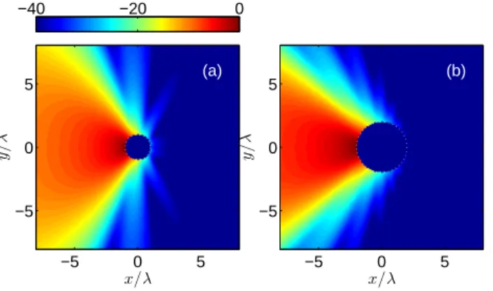
Figure 4: Longitudinal electric-field distribution generated by original sources with: (a)Ws=2λand (b)Ws=4λ. The inner regions with null radiation marks the minimum-sized cylinders containing the original sources.
which are similar to those found in (32). The main difference, apart the way the results were derived, is that in the case of the end-fire approach the excitation of the two radiating elements is the same apart for a phase shift, as usually done for this kind of arrays, whereas in the asymptotic case we still compute two different auxiliary current distributions. The possibility of gen-erating the information for the second layer from only a single one can be an asset when these data are measured rather than computed, e.g., from near-field facilities, as it would cut the measurement time by half.
The end-fire approach falls short of the global approach em-ployed in the optimal procedure as it does not aim to control the modal distortions. As shown in sec. 8, the residual error increases not only in the external region, but also in the internal one, by giving raise to a spurious focusing roughly covering the space occupied by the original source. Still, its overall ability in controlling the modal distortions is not much worse than that displayed by the asymptotic approximation.
8. Numerical results
The accuracy and effectiveness of the proposed approaches are assessed for the case of directive sources described by a linear current distributionJs(r )of lengthWs
Js(r ) = ˆze−jβxsin(πx/Ws)δ(y)δ(z) |x| ≤ Ws/2, (34) tapered toward its ends by a sinusoidal profile in order to pro-duce a dominant main lobe. Fig. 4 shows the electric field distribution they produce forWs=2λandWs=4λ. The am-plitudes of their modal coefficients are shown in Fig. 5. These configurations will be used throughout this section as references in evaluating the performance of layer coefficients derived by means of the optimal procedure (25), the asymptotic approxi-mation (32) or the end-fire approxiapproxi-mation (33).
All of the following results related to the optimal procedure involve the {βEm} as LS weights. Differences observed when
using the{βmH}are discussed in 8.4.
−15 −10 −5 0 5 10 15 0 5 10 15 20 25 m |γm | (a. u .) Ws= 4λ Ws= 2λ
Figure 5: Moduli of the modal coefficients{γm}for the case ofWs=2λand
Ws=4λ, serving as references.
8.1. Modal distortions
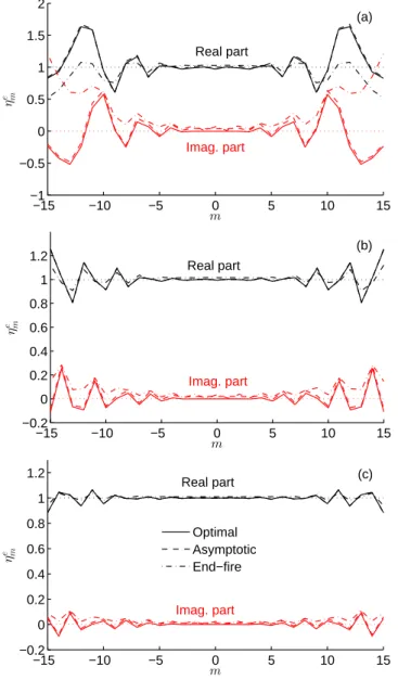
The question of how accurately two layers of electric currents can emulate these configurations can be assessed by means of several indicators. The first here considered, perhaps the most straightforward, is the set of modal distortions{ηm}for the ex-ternal and inex-ternal modal coefficients (16), which account for the imperfect reproduction of the original modal coefficients.
Some examples of results for the external distortions are given in Fig. 6, for three values of the inner radius R1; the
caseR1=Ws/2corresponds to the boundary of the minimum
cylinder containing the original source. Unless otherwise men-tioned in the rest of the paper, the second layer is always found at a distanced =λ/4outside the first one.
Fig. 6 shows that the end-fire approximation, though yielding a limited error over the modal indexesm where most of the radiated energy is found (see Fig. 5), actually presents a rapidly diverging error for|m| > 10. More fundamentally,ηem for the
end-fire case present a systematic error (bias) that will be shown in sec. 8.3 to have a major impact on the field topographies.
On the contrary, the optimal procedure has a very good per-formance for low-order modal indexes, where the{βm} coef-ficients enforce the most stringent conditions for the LS algo-rithm. It can be noticed how this performance comes to the expenses of a distortion that peaks for|m| = 12, though the dis-tortions are always bounded in these examples and have a minor impact on the overall results, since they apply to modes that are very weakly excited.
IncreasingR1 external distortions flatten out over a wider
range of modes for the three approaches, but the end-fire ap-proximation still displays a flat residual offset, as shown in Fig. 6(c). The differences in the performances of the three so-lutions are highlighted in Fig. 7, where|ηem−1|is shown to be only minimized in the case of optimal layer weights, while the asymptotic solution is only slightly better than the end-fire one. Concerning the internal distortions, Fig. 8 confirms that the results obtained with the optimal and asymptotic solutions are very similar, while the end-fire solution is again characterized by a flat offset that explains the appearance of a relatively im-portant inner radiation, as shown in sec. 8.3. Again, setting auxiliary currents further away from the original source region
−15 −10 −5 0 5 10 15 −1 −0.5 0 0.5 1 1.5 2 m η e m Imag. part Real part (a) −15 −10 −5 0 5 10 15 −0.2 0 0.2 0.4 0.6 0.8 1 1.2 Real part m η e m Imag. part (b) −15 −10 −5 0 5 10 15 −0.2 0 0.2 0.4 0.6 0.8 1 1.2 m η e m Imag. part Real part Optimal Asymptotic End−fire (c)
Figure 6: Real and imaginary parts of the overall external-field distortions{ηem}, computed in the caseWs=4λand∆R=λ/4for: (a)R1/Ws=1/2; (b)R1/Ws= 1and (c)R1/Ws=3/2.
strongly reduces the absolute value of the internal distortions; at the same time, the internal distortions also increase at a lower rate. It is worth observing that this trend is not shared by the end-fire solution, as its performance over low-order modes re-mains virtually unchanged.
8.2. Field errors on test surfaces
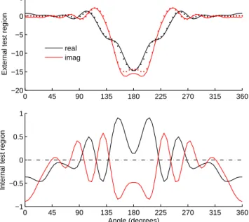
The modal distortions translate into errors on the electromag-netic field generated by the auxiliary sources, which can be measured on test surfaces as discussed in sec. 4. An exam-ple of typical results is given in Figs. 9 and 10, for the case
R1/Ws=1/2for end-fire and optimal procedures. In these two
cases, internal (external) test surfaces were defined at half a wavelength inside (outside) the innermost (outermost) layer of auxiliary electric currents. These results show that although the optimal procedure is expected to ensure a better performance,
−150 −10 −5 0 5 10 15 0.05 0.1 0.15 m |η e m − 1| Optimal Asymptotic End−fire
Figure 7: The distance|ηem−1|, computed in the caseWs=4λand∆R=λ/4 forR1/Ws=1. −150 −10 −5 0 5 10 15 0.2 0.4 0.6 m |η i m| Optimal Asymptotic End−fire
Figure 8: Absolute value of the overall internal-field biases{ηim}, computed in the caseWs=4λwith∆R=λ/4, forR1/Ws=1/2(black lines) andR1/Ws= 3/2(red lines).
the residual errors over the internal test surface can be locally stronger than by applying the end-fire approach. Moreover, the optimal procedure ensures that these errors are on average equal to zero, as opposed to the end-fire approximation; as it will be shown in sec. 8.3, these coherent deviations lead to residual focusing over the inner region.
Residual errors can be summarized by defining relative errors for the electric and magnetic fields
ǫ2E ,H(RT) =
e2E ,H(RT)
EE ,H , (35)
whereEE ,Hstands for the square of theL2norm of the electric (magnetic) field over the external test surfaceΣeT. Recalling (15), (17) and (21) ǫ2E ,H(RTe) = ∞ X m=−∞ |ηem−1|2|βE ,Hm (ReT)| 2 ∞ X m=−∞ |βE ,Hm (ReT)| 2 (36a) ǫ2E ,H(RTi) = ∞ X m=−∞ |ηim|2|βE ,Hm (RiT)| 2 ∞ X m=−∞ |βE ,Hm (RTe)| 2 , (36b) 7
0 45 90 135 180 225 270 315 360 −20 −15 −10 −5 0 5
External test region
0 45 90 135 180 225 270 315 360 −1 −0.5 0 0.5 1 Angle (degrees)
Internal test region
real imag
Figure 9: Real and imaginary parts of the longitudinal electric field forWs=4λ,
R1/Ws=1/2and∆R = λ/4, computed over cylindrical external (top figure) and internal (bottom figure) test surfaces, withRiT=R1−λ/2andReT=R2+λ/2, respectively. Results obtained under the end-fire approximation are shown as solid lines, reference results as dots.
whereEE ,Hare also taken as references for the internal errors, in order to assess the relative intensity of the residual field gen-erated over the inner regionΩ′i.
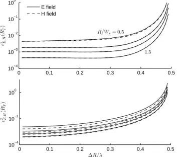
These figures of merit are shown in Figs. 11 to 13. Several trends can be pointed out. First of all, as∆Rapproachesλ/2, residual errors increase. This result can be understood by notic-ing that, under an asymptotic approximation, the field distribu-tions observed over two layers associated to each mode will be proportional one to the other if they are half a wavelength apart. Hence, rather than conveying complementary information that could be made to interfere, the two sets of auxiliary currents become increasingly redundant.
At the same time, as the ratioR1/Wsincreases, the errors
sys-tematically reduce. This behavior is easily understood within the framework introduced in sec. 6: in the limit fork0R1≫1,
all modal coefficients can be controlled at the same time. Fun-damentally for the same reason, errors on the magnetic and electric fields over the external test surface are practically iden-tical, while this is not true over the internal test surface, where the asymptotic expressions do not hold.
As expected, all errors are consistently lower for the optimal procedure. More importantly, the optimal procedure takes bet-ter advantage of a largerR1/Ws, with a faster rate of reduction
in the errors, when compared with the two approximate cases. The performance of the asymptotic approximation approaches that of the optimal procedure for largerR1/Ws, since the former
is correct in the limit fork0R1→ ∞.
0 45 90 135 180 225 270 315 360 −20 −15 −10 −5 0 5
External test region
0 45 90 135 180 225 270 315 360 −2 −1 0 1 2 Angle (degrees)
Internal test region
real imag
Figure 10: Same configuration as in Fig. 9. Results obtained with optimal layer weights.
8.3. Field topographies
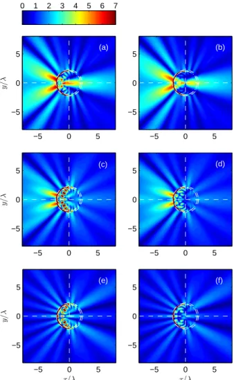
An example of the field topographies generated by two-layer auxiliary currents is shown in Fig. 14, emulating the linear source (34) whenWs=4λ. The three sets of electric and mag-netic field distributions are to be compared to the original case reproduced in Fig. 4(b).
Differences between the performance of the three solutions are shown in Figs. 15 and 16, as percentages of the peak field amplitude observed over the external regionΩ′e; two values of R1/Wsare considered, namely0.5and1.5. Independently from
the dimensions of the shell-region, it is found that the end-fire approach always leads to a residual (coherent) focusing within the inner regionΩ′i, as opposed to an incoherent interference pattern observed with the other two solutions. Errors in the external region drop when applying the optimal procedure. 8.4. Cross comparisons
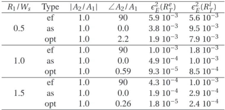
This section draws some cross comparisons between the per-formance as already presented and the layer weights that gen-erated them. The first such comparison is presented in Table 1 where the layer weights applied for the three methods are sum-marized. The weights{Al}are presented in a normalized form,
asA2/A1.
We first need to recall that the weights of the approximate so-lutions only depend on the relative distance between the layers. By the same token, the approximate solutions are by definition only operating by phase-shifting the individual radiations from the auxiliary layers. Conversely, for the optimal procedure, this property is never explicitly enforced; the fact that all the re-sults in Table 1 involve|A1/A2| =1is therefore worth noticing,
as it implies that there is no need for amplitude-compensation schemes.
0 0.1 0.2 0.3 0.4 0.5 10−6 10−4 10−2 100 ǫ 2 E,H (R e T) 0 0.1 0.2 0.3 0.4 0.5 10−5 10−3 10−1 ∆R/λ ǫ 2 E,H (R i T) E field H field 1.5 1.0 0.75 R/Ws= 0.5
Figure 11: Comparison between relative errors on the electric and magnetic fields over the external test surfaceΣeT(upper graph), withRTe=R + ∆R + λ/2 and the internal test surfaceΣiT(lower graph), withRTi =R −λ/2, for a varying distance∆Rbetween two current layers. Four values ofR/Wsare considered, equal to 0.5, 0.75, 1.0 and 1.5. Results for a source widthWs=4λ, optimal layer weights.
As a consequence, it appears that the major differences in the performance between the approximate and optimal proce-dures are in fact due to minor differences in the phase-shift an-gle enforced between the layers. While the asymptotic solution requires an in-phase radiation of the two layers, the optimal one spans phase-shift angles between 0.26 and 2.2 degrees, for
R1/Ws passing from 1.5 to 0.5. Correspondingly, the external
error decreases more steeply for the optimal procedure, with a relative improvement of about a factor 2 to 10 with respect to the asymptotic solution.
Table 2 seeks to point out how the choice of electric or mag-netic weights{βm}affects the performance of the optimal pro-cedure. To this end, the layer weights and errors were computed for the two choices of{βm}: all the quantities in Table 2 noted by the letter ‘R’ stand for the ratio of results obtained by choos-ing{βHm}and those obtained with{βEm}; e.g.,RAis the ratio of A2/A1 obtained in the two cases, of which only the marginal
phase-shift angle is shown, as expressed in degrees. All other ratios are self-explaining.
It can be concluded that the kind of{βm}chosen has little im-pact on the error metrics on the external test surface, with vari-ations of the order of the percent point; this trend is reinforced when passing fromWs=2λtoWs=4λ. Moreover, the same conclusions hold for both electric and magnetic field external errors. As opposed to these conclusions, the internal errors are more sensitive to the choice of the{βm}weights.
The asymptotic proportionality between{βEm}and{βmH},
dis-cussed in sec. 5, is confirmed, with residual phase-shift angle ofRApassing from1.8to0.23degrees forWs=2λ.
A last comparison is needed between the performance of the
0 0.1 0.2 0.3 0.4 0.5 10−4 10−3 10−2 10−1 100 ǫ 2 E,H (R e T) 0 0.1 0.2 0.3 0.4 0.5 10−5 10−3 10−1 ∆R/λ ǫ 2 E,H (R i T) E field H field 1.5 1.0 0.75 R/Ws= 0.5
Figure 12: Same configuration as in Fig. 11; results for the asymptotic solution.
R1/Ws Type |A2/A1| ∠A2/A1 ǫ2E(ReT) ǫ2E(RTi) 0.5 ef 1.0 90 5.9 10−3 5.6 10−3 as 1.0 0.0 3.8 10−3 9.5 10−3 opt 1.0 2.2 1.9 10−3 7.9 10−3 1.0 ef 1.0 90 1.0 10−3 1.8 10−3 as 1.0 0.0 4.9 10−4 1.0 10−3 opt 1.0 0.59 9.3 10−5 8.5 10−4 1.5 ef 1.0 90 4.3 10−4 1.0 10−3 as 1.0 0.0 1.9 10−4 2.9 10−4 opt 1.0 0.26 1.8 10−5 2.4 10−4
Table 1: Absolute value and phase shift of the relative weightA2/A1, for the three methods of computation of the layer weights, for the caseWs=4λand ∆R = λ/4. The corresponding relative errorsǫ2E(RT)give a measure of how such small adjustments in the layer weights lead to large differences in the quality of reconstruction of the field distribution. Shorthand notations are used for the end-fire (ef), asymptotic (as) and optimal (opt) solutions.
external-field optimization and the joint internal-external one. It was suggested in sec. 6 that, asymptotically, reproducing the original radiation over the external region must pass for a null radiation over the internal region. As such, a joint optimization can be regarded as redundant, as long asL ≪ M. In this re-spect, the results shown in Fig. 17 support this analysis, since the internal modal distortions are practically unmodified when switching between the two optimization strategies. The joint optimization should therefore be considered only in those cases whereL ≃ M.
9. Conclusions
This paper analyzed the possibility of defining auxiliary cur-rent distributions, extending the idea of Love’s equivalent theo-rem to the case of electric-only currents. Rather than proceed-ing through the definition of an inverse problem, our proposal is 9
0 0.1 0.2 0.3 0.4 0.5 10−4 10−3 10−2 10−1 100 ǫ 2 E,H (R e T) 0 0.1 0.2 0.3 0.4 0.5 10−4 10−2 100 ∆R/λ ǫ 2 E,H (R i T) E field H field R/Ws= 0.5 1.5
Figure 13: Same configuration as in Fig. 11; results for the end-fire approxima-tion. R1/Ws Ws/λ ∠RA Rǫ,eE Rǫ,iE R H ǫ,e Rǫ,iH 0.5 2 1.79 1.03 1.25 1.01 0.543 4 0.447 0.969 1.02 0.951 0.987 1.0 2 0.499 1.05 1.25 1.04 0.511 4 0.119 1.01 0.991 1.01 0.975 1.5 2 0.234 1.05 1.26 1.05 0.505 4 0.0553 0.994 1.01 0.993 0.973
Table 2: Comparison of the performance of the optimal procedure when ap-plying magnetic or electric weights{βm}. All quantities represent the ratio of results and metrics obtained with the magnetic weights normalized to those obtained with electric weights. Refer to sec. 8.4 for details about the notations.
based on a hybrid solution, keeping the electric current distribu-tion defined by Love’s theorem. The role of magnetic currents is taken over by further layers of electric currents weighted in such a way as to approximate the results expected for the equiv-alence theorem. The resulting procedure ensures a good perfor-mance, with residual errors of the order of a few percent points.
Acknowledgement
Part of the work here reported was funded by the French National Research Agency through the grant ANR-12-ASTR-0005, within the framework of the 2012 ASTRID program.
References
[1] A. Love, The integration of the equations of propagation of electric waves., Proceedings of the Royal Society of London 68 (442-450) (1901) 19–21.
[2] H. MacDonald, The integration of the equations of propagation of electric waves, Proceedings of the London Mathematical Society 2 (1) (1912) 91– 95. y/ λ (a) −5 0 5 −5 0 5 −40 −20 0 (b) −5 0 5 −5 0 5 (e) x/λ y/ λ −5 0 5 −5 0 5 x/λ (f) −5 0 5 −5 0 5 y/ λ (c) −5 0 5 −5 0 5 (d) −5 0 5 −5 0 5
Figure 14: Field distributions generated by two-layer auxiliary currents with
R1=Ws/2and spacing∆R = λ/4, for the source (34) withWs=4λ. The mod-ulus of the longitudinal electric (left column) and transverse magnetic (right column) fields, expressed in dB and normalized to their peak value, for the (a)-(b) end-fire, (c)-(d) asymptotic and (e)-(f) optimal solutions. The auxiliary-current layers are shown as dashed circles.
[3] W. Smythe, The double current sheet in diffraction, Physical Review 72 (11) (1947) 1066.
[4] R. Harrington, Time-Harmonic Electromagnetic Fields, McGraw-Hill, New York, NY, 1961.
[5] S. R. Rengarajan, Y. Rahmat-Samii, The field equivalence principle: Il-lustration of the establishment of the non-intuitive null fields, Antennas and Propagation Magazine, IEEE 42 (4) (2000) 122–128.
[6] S. Schelkunoff, Some equivalence theorems of electromagnetics and their application to radiation problems, Bell Syst. Tech. J 15 (1) (1936) 92. [7] E. Martini, G. Carli, S. Maci, An equivalence theorem based on the use
of electric currents radiating in free space, Antennas and Wireless Propa-gation Letters, IEEE 7 (2008) 421–424.
[8] F. Las-Heras, T. K. Sarkar, Radial field retrieval in spherical scanning for current reconstruction and nf-ff transformation, Antennas and Propaga-tion, IEEE Transactions on 50 (6) (2002) 866–874.
[9] J. Colinas, Y. Goussard, J. Laurin, Application of the Tikhonov regular-ization technique to the equivalent magnetic currents near-field technique, Antennas and Propagation, IEEE Transactions on 52 (11) (2004) 3122– 3132.
[10] P.-A. Barriere, J. Laurin, Y. Goussard, Mapping of equivalent currents on high-speed digital printed circuit boards based on near-field mea-surements, Electromagnetic Compatibility, IEEE Transactions on 51 (3)
y/ λ (c) −5 0 5 −5 0 5 x/λ y/ λ (e) −5 0 5 −5 0 5 x/λ (f) −5 0 5 −5 0 5 y/ λ (a) −5 0 5 −5 0 5 0 1 2 3 4 5 6 7 (b) −5 0 5 −5 0 5 (d) −5 0 5 −5 0 5
Figure 15: Intercomparison between the errors of the three synthesis methods, expressed as percentage of the peak amplitude of the field distributions external to the auxiliary-current layers, forR1/Ws=1/2(cf. Fig. 14). Axial electric (left column) and transverse magnetic (right column) error distributions for the (a)-(b) end-fire, (c)-(d) asymptotic and (e)-(f) optimal solutions.
(2009) 649–658.
[11] T. F. Eibert, E. Kaliyaperumal, C. H. Schmidt, et al., Inverse equivalent surface current method with hierarchical higher order basis functions, full probe correction and multilevel fast multipole acceleration, Progress In Electromagnetics Research 106 (2010) 377–394.
[12] J. Van Bladel, Electromagnetic fields, IEEE, 2007.
[13] J. E. Hansen, Spherical near-field antenna measurements, Vol. 26, IET, 1988.
[14] W. C. Chew, E. Michielssen, J. Song, J. Jin, Fast and efficient algorithms in computational electromagnetics, Artech House, Inc., 2001.
[15] C. L. Lawson, R. J. Hanson, Solving least squares problems, Vol. 161, SIAM, 1974. (a) y/ λ −5 0 5 −5 0 5 0 1 2 3 (b) −5 0 5 −5 0 5 y/ λ (c) −5 0 5 −5 0 5 (d) −5 0 5 −5 0 5 x/λ y/ λ (e) −5 0 5 −5 0 5 x/λ (f) −5 0 5 −5 0 5
Figure 16: Same as in Fig. 15, for the caseR1/Ws=3/2.
−8 −6 −4 −2 0 2 4 6 8 0 0.01 0.02 0.03 0.04 0.05 m |η i m| Ext. opt. Joint opt.
Figure 17: Absolute value of the overall internal-field modal distortions{ηim}, computed in the caseWs=4λwith∆R=λ/4, forR1/Ws=1/2(black lines) andR1/Ws=3/2(red lines).