Design and Control of a Soft Biomimetic Batoid
ARCHIVES
Robt
SACHUsETTS INSTITERobotOFTCNLG
by
JUN
2
5 2013
Audren Damien Prigent Cloitre
B.S., Arts et Metiers ParisTech (2010)
7
RA ES Submitted to the Department of Mechanical Engineeringin partial fulfillment of the requirements for the degree of Master of Science in Mechanical Engineering
at the
MASSACHUSETTS INSTITUTE OF TECHNOLOGY
June 2013
@
Massachusetts Institute of Technology 2013. All rights reserved.Author ...
Certified by...
Department of Mechanical Engineering
May 20, 2013
Nicholas M. Patrikalakis Kawasaki Professor of Engineering
/.... Thesis Supervisor
Certified by...
Kamal Youcef-Toumi
1</
I
rofesso of Mechanical Engineering-
I.* Thesis SupervisorCertified by ... ,
Pablo Valdivia Y Alvarado
- Ptesearch Scientist
Thesis Supervisor A ccepted by ... :..lr ... ...
David E. Hardt Chairman, Department Committee on Graduate Theses
Design and Control of a Soft Biomimetic Batoid Robot
by
Audren Damien Prigent Cloitre
Submitted to the Department of Mechanical Engineering on May 20, 2013, in partial fulfillment of the
requirements for the degree of
Master of Science in Mechanical Engineering
Abstract
This thesis presents the work accomplished in the design, experimental characteriza-tion and control of a soft batoid robot. The shape of the robot is based on the body of the common stingray, Dasyatidae, and is made of soft silicone polymers. Although soft batoid robots have been previously studied, the novelty brought by the present work centers around autonomy and scale, making it suitable for field operations.
The design of the robot relies on the organismic consideration that the stingray body is rigid at its center and flexible towards its fins. Indeed, all mechanical and electrical parts are inside a rigid shell embedded at the center of the robot's flexible body. The silicone forms a continuum which encases the shell and constitutes the two pectoral fins of the robot. The core idea of this design is to make use of the natural modes of vibration of the soft silicone to recreate the fin kinematics of an actual stingray. By only actuating periodically the front of the fins, a wave propagating downstream the soft fins is created, producing a net forward thrust.
Experiments are conducted to quantify the robot's swimming capabilities at dif-ferent regimes of actuation. The forward velocity, the stall forces produced by the robot when it is flapping its fins while being clamped, and the power consumption of the actuation are all measured. The peak velocity of the robot is 0.35 body-length per second and is obtained for a flapping frequency of 1.4 Hz and a flapping amplitude of 300. At a flapping frequency of 2 Hz, and an amplitude of 30', the maximum stall forward force of the robot averages at 45 Newtons and peaks at 150 Newtons. Other data collected is used to better understand the hydrodynamics of the robot.
Thesis Supervisor: Nicholas M. Patrikalakis Title: Kawasaki Professor of Engineering Thesis Supervisor: Kamal Youcef-Toumi Title: Professor of Mechanical Engineering Thesis Supervisor: Pablo Valdivia Y Alvarado Title: Research Scientist
Acknowledgments
I wish to acknowledge the support of my three advisors, Prof. N. M. Patrikalakis,
Prof. K. Youcef-Toumi and Dr. P. Valdivia Y Alvarado. I also wish to thank Prof. M.
S. Triantafyllou for granting me access to the MIT Tow Tank laboratory where I was
able to realize my experiments. I want to mention how lucky I feel, to have worked with people that showed me nothing but patience, understanding and support. Prof. Patrikalakis, Prof. Youcef-Toumi, Dr. Valdivia Y Alvarado, thank you.
I would like to thank my fellow collegues and labmates who helped in assembling
or operating the robot: Dilip Thekkoodan, Vignesh Subramaniam, Bruce Arensen and Katherine Martinez. I also acknowledge the help of my friends who assisted me during experiments: Maxime Cohen, Daniel Dadon, Ryan Iutzi, Matthieu Monsch, Kevin Spencer, Gabriel Bousquet, Lydia Jackson, Heather Beem and Stephanie Chin.
My thanks go to Dr. G. Weymouth who graciously offered to use his swimming pool
in Singapore for the early experiments with the robot. In general, all the members of the WAVES laboratory, the Tow Tank laboratory and the Mechatronics Research Laboratory (MRL) have been fantastic companions, both for their scientific input and their friendship.
This thesis is dedicated to my family who has been with me in this adventure. The principles learned from my parents have never felt so important and so appre-ciated when I arrived in this new country. Their devotion to educate their children and make sure they succeed as adults is inspiring, a model. My thoughts are with my sister too. She's always been there when I needed her. Maman, Papa, Morgane, merci.
This research was supported by the National Research Foundation of Singapore through the Singapore-MIT Alliance for Research and Technology's Center for Envi-ronmental Sensing and Modeling (CENSAM) IRG research program.
Contents
1 Introduction
1.1 Motivations for Studying Underwater Soft Biomimetic Robots . . . . 1.1.1 A Need for Autonomous Underwater Vehicles . . . .
1.1.2 Soft Biomimetic Robots vs. Traditional Robots . . . .
1.1.3 The WAVES lab at CENSAM . . . . 1.1.4 Summary of the Motivations for the Creation of a Soft Biomimetic
B atoid Robot . . . . 1.2 P rior A rt . . . . 1.2.1 Oscillating Batoid Robots . . . . 1.2.2 Undulating Knife Fish Robots . . . .
1.2.3 Undulating Stingray Robots . . . ..
1.3 Statement of Objectives and Presentation of the Thesis . . . . 2 Theoretical Work
2.1 Introduction . . . . 2.2 The Pair Material - Manufacturing Process .
2.3 The Design of the Actuation . . . .
2.4 Trajectory Control . . . . 2.4.1 M odel . . . . 2.4.2 Feedback and Controller . . . .
3 Prototype
3.1 Components and Assembly. . . . .
15 15 15 16 18 18 19 20 20 21 21 23 . . . . 2 3 . . . . 2 4 . . . . 2 6 . . . . 3 3 . . . . 33 . . . . 36 41 41
3.1.1 Power ... 3.1.2 Sensors. . . . . 3.1.3 Controllers. . . . . . 3.1.4 Communication . . . 3.1.5 Housing . . . . 3.2 Actuation . . . . 3.3 Control of the Actuators 4 Experiments
4.1 Introduction . . . .
4.2 Power Acquisition. . . . . . 4.2.1 Experimental Set-up 4.2.2 Results and Analysis 4.3 Velocity Acquisition. . . . .
4.3.1 Experimental Set-up 4.3.2 Results and Analysis 4.4 Force Acquisition . . . .
4.4.1 Experimental Set-up 4.4.2 Results and Analysis
. . . . 4 1 . . . . 4 2 . . . . 4 3 . . . . 4 4 . . . . 4 4 . . . . 4 9 . . . . 5 2 57 . .. . . . 5 7 . .. . . . 5 8 . .. . . . 5 8 . .. . . . 5 8 . . . . 6 1 . . . . 6 1 . . . . 6 2 . . . . 6 5 . . . . 6 5 . . . . 6 6
5 Conclusions and Recommendations
A MatLab@ Implementation of the Actuator Dynamical Model
B MatLab@ Implementation of the Digital Vision Tracking Algorithm 69 75 81 C Derivation of the equations of motion of the model of the robot for
trajectory control 91
C.1 Force Derivations . . . . 91 C.2 The Added Mass Effect . . . . 94
List of Figures
1-1 The three biological models the robots presented in the Prior Art sec-tion are based upon . . . . 19 2-1 Presentation of the main elements of the robot . . . . 24 2-2 Left: Bottom view of the mold. Right: Top view of the mold . . . . . 25
2-3 Positive of the mold made out of a puzzle of 3D-printed parts . . . . 25
2-4 Side view of the model of the robot's fin . . . . 26 2-5 Side view of the Free-Body Diagram of the actuation of the robot. . . 28
2-6 Expected power consumption at the input of the motor (in solid blue)
and at the output gear (in dashed blue) as well as the output torque (in red) for an input flapping amplitude of 30 degrees, and at a frequency of2 Hz. ... ... 31 2-7 Top-view schematic of the model of the robot. Forces are in red, the
velocity of the robot is in green. . . . . 33 3-1 Schematic of the electric circuit that delivers the power to the actuator. 42
3-2 On the left: GPS unit. At the center, Inertial Measurement Unit. On the right: Encoder . . . . 42
3-3 On the left: The Electronic Speed Controller. On the right: the mbed
NXP LPC1768 . . . . 43 3-4 On the left: center part of the shell as it is out of the 3D printer. On
the right: the three parts of shell . . . . 46
3-6 Exploded view of the robot. The robot is presented upside down to show the inside of the shell. . . . . 48
3-7 Capabilities of the motor in terms of torque and angular velocity . . . 49
3-8 On the left: exploded view of the motor and gearbox assembly. On
the right: Picture of the gearbox and the motor. The flapper is not yet mated with the output gear. The coin is an American quarter. . . 51 3-9 Control loop of one actuator . . . . 52 3-10 Control loop of one actuator . . . . 53 3-11 Pole/Zero map of the controlled actuator . . . . 53 3-12 Measurements of the actual performance of the actuator control . . . 55
4-2 On the left: ESCON 36/3 from Maxon Motor. On the right: AttoPilot Voltage and Current Sense Breakout . . . . 58
4-1 Presentation of the input variable 6(t). The white dotted line marks the horizontal reference; the red line follows the flapper. . . . . 59
4-3 RMS values of the power consumed by one motor for various flapping frequencies and amplitudes. . . . . 60
4-4 Schematic side view of the set-up for the velocity acquisition experiment. 61 4-5 Picture sequence of the velocity acquisitions. The yellow crosses that
appears on top of the red markers were added by the MatLab@ program 63 4-6 Collection of the measured mean speed of the robot for two flapping
amplitudes and seven flapping frequencies. Three measurements were made per flapping configuration . . . . 64 4-7 On the left, schematic side view of the set-up for the force acquisition
experiment. On the right, pictures of the robot mounted on the force sensor. . . . . 65
4-8 Raw result of one forward force acquisition. In this acquisition, the robot is flapping at 30 degrees of amplitude and 2 Hz. . . . . 66
4-9 Mean of the forward force, for a flapping amplitude of 20 and 30 de-grees and a frequency ranging from 0.8 Hz to 2 Hz. Each data point corresponds to the mean of three acquisitions done at the same flapping amplitude and frequency. . . . . 67 C-1 Digital rendering of the shape of the robot (in green) and the spheroid
approximation (in blue) for the added mass effect. Values of the pa-rameters given in table C.1. . . . . 95
List of Tables
2.1 Values of the parameters used in the model of the actuator . . . . 27
2.2 Values of the parameters used in the model for trajectory control . . 34 3.1 D esign table . . . . 45
C. 1 Values of the parameters used for the derivation of the added mass
Chapter 1
Introduction
1.1
Motivations for Studying Underwater
Soft Biomimetic Robots
1.1.1
A Need for Autonomous Underwater Vehicles
The ocean is one of the last territories on Earth humans have yet to fully explore. According to the National Geographic
[1]
and the National Oceanic and Atmospheric Association (NOAA)[2],
less than 10% of the sea floor has ever been seen by a human eye. This can be explained by two reasons:* The sea floor can lay at depths as low as 10 km below the sea level, in the Mariana trench. Building a submarine capable of bearing the pressure of the water at this kind of depth is a challenge that only few groups try to overcome
[3]
e The sea represents 70% of the earth's surface. It would take tremendous human
resources if the exploration were to be done by humans and not by machines. Autonomous Underwater Vehicles, (AUVs), present an alternative to a daunting challenge: human exploration of the sea. AUVs are designed to work on their own; giving only occasional feedback on their missions to a remote human operator. They
can carry biological sensors to monitor the quality of the water of a given area [4] or a sonar to map the terrain of the sea floor or detect specific objects lying on the sea bed [5]. Because they are versatile and do not require a human on board, they are a promising solution to better understand the sea; an environment that can quickly become hostile to a human explorer.
1.1.2
Soft Biomimetic Robots vs. Traditional Robots
Traditional AUVs travel underwater using propellers or by changing their buoyancy. Here are presented the three most common designs of AUVs:
" One buoyancy tank generates a sawtooth-like vertical motion by periodically
emptying and filling itself with water. Rigid fins orient the AUV vertically and, in some designs, also horizontally. These AUVs are called sea-gliders [6]. * One propeller at the back of the AUV generates the thrust. Rigid actuated fins
orient the AUV in the vertical and horizontal planes [7]. This is a torpedo-like design.
" Several propellers are used both to generate the thrust and to direct the AUV [8]. AUVs using this design are called hovering AUVs (HAUVs).
* AUVs use the energy from the waves of the ocean to propel themselves. An example of this design can be found with the company Liquid Robotics and their wave glider [9].
The first type is generally used to run longer missions, in open waters, where agility is not the prior concern. They can be deployed for missions lasting several months and can cover hundreds of miles. The second type is typically used for mid-range operations, both in terms of duration and distance. They are well suited for an all-day-long mission where data need to be collected in an area ranging from a few hundred meters to a few tens of kilometers. The last type is used for short missions where high maneuverability is critical; typically for boat hull inspections. They are
designed to stay in an area a few hundred meters wide and to hover still at one loca-tion when needed.
Biomimetic Robots can complement the capabilities of traditional AUVs as the former aim to be both efficient for long distance travels and to offer high maneuver-ability. One drawback of traditional AUVs is that they are usually well suited for only one specific domain of operations. Few solutions exist for hybrid missions of long distance survey and confined space maneuvering. The expected gain from mimicking fish locomotion is to obtain the same swimming efficiency and low-speed agility they benefit.
There are two main approaches to mimic the locomotion of a fish:
" Several rigid links are actuated with respect to one another. They discretize
the body of the fish and approximate its curvature by actuating each link with respect to one another. This rigid-link approach has been widely used among research groups working on fish locomotion after it was first introduced by Barrett's Master thesis in 1994 [10] and by Triantafyllou et al. in 1995 [11].
" The fins or the body of the robot are made out of a flexible material whose
material properties match the ones of the mimicked animal. Only one actua-tor is used to excite the flexible material whose modes of vibration match the kinematics of the fish [12].
The work presented in this thesis follows the principles developed by Valdivia Y Alvarado [13]. By reducing the number of actuators, soft robotics aims to reduce the power consumption of the robot and its control complexity. Moreover, a simpler system is more likely to be more robust; a key factor to having a successful field deployable robot.
1.1.3
The WAVES lab at CENSAM
The soft biomimetic stingray will ultimately find its place in a larger network of au-tonomous robots. This work was funded by the National Research Foundation (NRF) of Singapore at the Center for ENvironmental Sensing And Modeling (CENSAM).
As its name indicates, CENSAM's goal is to develop tools for urban and coastal en-vironmental sensing and modeling in Singapore. Within this center, the Water and Air Vehicles for Exploration and Sensing (WAVES) lab provides environmentalists with aerial, surface and underwater vehicles that serve as deployable platforms to transport the necessary sensors.
The current AUVs used for underwater acquisitions are part of the second category of traditional AUVs previously introduced: torpedo-like AUVs. Although this plat-form proved to be very successful in completing early missions [14]; its propeller does create a turbulent wake that can disturb the local marine flora and fauna. A fish-like robot would create similar wakes as the other fishes, and disturb less its immediate environment.
1.1.4
Summary of the Motivations for the Creation of a Soft
Biomimetic Batoid Robot
"
Researchers need a new kind of AUV that can achieve both agile motions in confined spaces and efficient locomotion over long distances." A soft-body approach that exploits flexible body natural modes requires less
actuators than a rigid-link approach. The expected gain is to decrease power consumption and control complexity.
" An AUV traveling underwater like a fish could create less turbulent and
disturb-ing wakes than propeller-based AUVs; allowdisturb-ing for flora and fauna observations.
" A stingray was chosen as a model for the robot for two reasons: (1) its central
body is naturally rigid and can be used to contain all the necessary components and (2) the coastal sea of Singapore is one of the natural habitats of the stingray.
Oscillating
t[
Undulating
Manta ray Stingray Knife fish
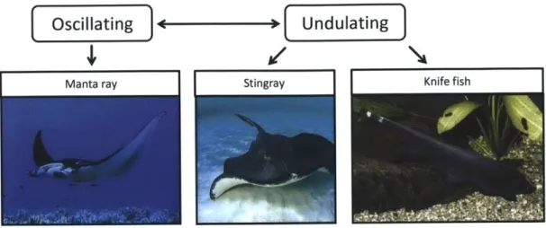
Figure 1-1: The three biological models the robots presented in the Prior Art section are based upon
1.2
Prior Art
This section focuses on reviewing the work achieved in the field of underwater biomimetic robotics. As this field is vast, only the designs similar to the one discussed in this thesis are addressed in this section. Similarities are evaluated in terms of swimming mechanisms and shape of the robot. Since the robot discussed in this thesis is based on the Dasyatidae Taeniura (a genus of stingray), other robots based on batoid rays are considered in this section. Those robots are generally based on the manta ray or the cownose ray, both of which, use an oscillatory mode of swimming. This is different from the swimming mechanism of the stingray which is undulatory. The difference between the two modes of swimming is studied by Rosenberger in [15]. Undulatory swimming mechanisms pass multiple waves down the fin or the body as opposed to oscillatory mechanisms that use a flapping motion. Finally, Although knife fishes are not batoid rays, robots designed based on the knife fish model are also presented in this section as the knife fish swimming mechanism is also undulatory. Fig. 1-1 shows the three biological models the robots considered in this section are based upon.
1.2.1
Oscillating Batoid Robots
The manta ray has been the base of numerous designs among the robotic community. Parson et al. [16] explains that the manta ray shows better turning performances than the stingray. However, results are obtained for banked turns, when the fish has already gained momentum from a linear acceleration phase prior to the turn. It can be argued that undulatory motion can provide better performances when the fish needs to rotate on a spot, without any prior velocity.
Moored and Bart-Smith proposed a novel actuator based on tensegrity structures to mimic the motion of the wing of a manta ray [17] [18]. Zhou and Low proposed a design where each fin of a manta ray is approximated by three rays, actuated independently [19]. Finally, the cownose ray is the base of an interesting design by Gao et al. [20]. This robot possesses only two actuators and the fins are made of compliant silicone rubber. This is very similar to the design approach taken for the robot presented in this thesis; at the difference that the motion of the cownose is oscillatory unlike the one of the stingray, which is undulatory.
1.2.2
Undulating Knife Fish Robots
The knife fish is an interesting system as it can be approximated as a rigid body with an undulating anal fin for propulsion. This biological model was first introduced
by MacIver et al. [21]. Like the robot presented in this thesis, the mechanical and
electrical components of the robot are contained within the body, eliminating any constraints for the deformation of the fin.
Siahmansouri et al. [22], and Low [23] use this feature to embed a buoyancy tank in the body and enable depth control. The hydrodynamic behavior of the undulating fin is addressed by Curet et al. [24] who study the effect of counter-propagating waves travelling the fins simultaneously. The thrust generation is explored by Epstein et al. [25] where the thrust is measured for various input flapping frequencies and ray
deflections.
1.2.3
Undulating Stingray Robots
The particularity of the stingray is that though its physiology is close to the one of the manta ray; its undulatory swimming mechanism brings it closer to the knife fish. Low, who has already been cited for his work on a robotic knife fish, focuses also his work on mimicking the stingray [26] [27]. His robot is autonomous and the fins are made out of an assembly of crank-sliders subsystems, individually actuated by servomotors. The final machine contains a total of 20 servomotors in order to actuate the two fins. A high number of actuators is generally the cause of an increase in control complexity, an increase of power consumption and a low mean-time-to-failure value. This motivates the change in strategy adopted by Valdivia Y Alvarado. His robotic stingrays were made out of a soft material and only require one actuator per fin [28]. They successfully swim and the wake they generate was studied in order to better control their motion [29]. However, these robots were not yet fully autonomous.
1.3
Statement of Objectives and Presentation of
the Thesis
The design of the soft biomimetic batoid robot is the first objective of this Master thesis. Since the robot has to be autonomous, the design uses onboard power supply, control electronics and navigation sensors. It is designed to be at the same scale as an adult stingray in order to be deployed in the wild. The preliminary work on the control of the robot is derived so as to allow it to swim at the surface of the water, following a set of predetermined way points. Experiments characterizing the robot's performance are conducted. The performance is assessed in terms of forward speed, stall forward force, and power consumption.
manufacturing the robot. This covers all design and control considerations. A third chapter details the prototype construction. The experiments conducted on the robot and their analysis are presented in the fourth chapter. A conclusion and statement of future work mark the end of the thesis.
Chapter 2
Theoretical Work
2.1
Introduction
This section presents the preliminary work achieved prior to building any prototype. Although several prototypes were designed and assembled, all of them are based on the same core elements. The main elements that make up the robot are shown in Fig. 2-1:
* The tail: Separated from the body, it has no other functionality at this stage than preserving the aesthetics of the robot.
" The body: It is the ensemble shell + silicone. The silicone is one
that encases the shell and forms the fins.
" The fins: They are the propulsive elements of the robot. Each one towards the front of the robot by a rigid flapper.
" The shell: It is a sealed container that carries all the electronics and components of the robot. It is cast inside the silicone.
continuum
is actuated
mechanical
The specifications that led to choose this design structure are listed as follows: * Materials: Make use of a soft material to reduce the number of actuators.
Figure 2-1: Presentation of the main elements of the robot
e Robot autonomy: The robot has to be autonomous in terms of power, sensing
and control.
All these concerns will be addressed and their solutions are presented in the
fol-lowing subsections:
" The Pair Material - Manufacturing Process
" Design of the Actuation " Trajectory Control
2.2
The Pair Material
-
Manufacturing Process
It is unusual to start a design summary by the manufacturing process. One could think this should be dealt at the end, once the design is finalized and ready for pro-duction. In our case, the manufacturing process itself is the main design limitation
Figure 2-2: Left: Bottom view of the mold. Right: Top view of the mold
Figure 2-3: Positive of the mold made out of a puzzle of 3D-printed parts because of the nature of the material used to build the robot.
It was a design specification to build the robot out of a soft material. Using the lessons learned from Dr. Valdivia Y Alvarado's thesis [13], silicone polymers were cho-sen as they offer suitable material properties in terms of density, elasticity (Young's modulus) and viscosity. Since silicone is not easy to form once cured; it should be formed during its liquid state by casting it in a mold.
The size of the mold determines the size of the robot. It was thus a main concern to get the mold as big as feasible; yet keeping it light enough to be handled manually
by one operator. Mold machining using standard materials (resin, plastics or metals)
would result in a heavy mold (if using metals) or a fragile one (if using resin) that would not be practical to use by a stand-alone operator. However, the solution of thermoforming a sheet of plastic on a model of the robot allows to build several light-weight molds, with respectable tolerances and that are bendable so as to ease the
P2 Flapper L Ab~~~P woo________ CZ ^^^6 = Asin(27rft) p3, 0 K Water density: p C
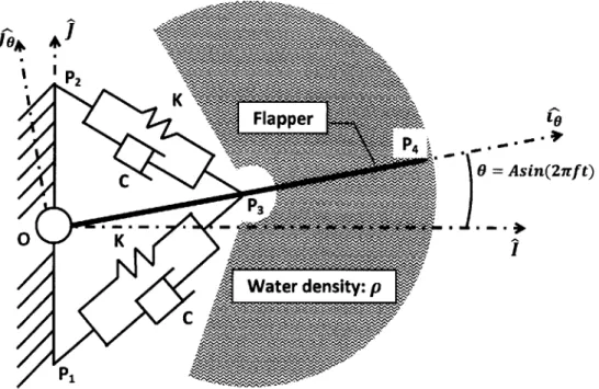
Figure 2-4: Side view of the model of the robot's fin
demolding process. The biggest thermoforming machine at MIT has a working area of 24 by 24 inches; the body of the robot was then designed to fit in a 24 inch wide diameter. According to Nelson [30], and White et al. [31], this diameter corresponds to an average adult size for a common stingray like the Dasyatidae Taeniura. Pictures of the molds are presented in Fig. 2-2 and the 3D-printed parts used to thermoform the molds is depicted in Fig. 2-3.
2.3
The Design of the Actuation
The model of the actuation of the stingray fin is based on the assumption that a rigid plate, the flapper, is cast in silicone and is prescribed to rotate about a point 0 inside the body, alternating its sense of rotation periodically. The flapper is the rigid link that connects point 0 and point P4, as shown in 2-4. The flapper is attached to
the shell at the pivot point 0 and its position is parameterized by 0(t) which defines the rotation between the ground frame (0,
Z,
J, K) and the frame attached to the flapper (0,i,.jo, ko = K) .Table 2.1: Values of the parameters used in the model of the actuator
Parameter Name Value
Height of bottom silicone OP1 4 cm
Height of top silicone OP2 4 cm
Distance to the attachment point of the silicone OP3 6 cm
Length of the flapper OP4 12 cm
Width of the flapper w 10 cm
Drag coefficient of the flapper C 2 Spring constant of the silicone K 3883 N.m
Damper constant of the silicone C 277 N.s/m
Young's modulus of the silicone E 0.07 MPa
Viscosity of the silicone P 50 N.s/m 2
Density of the water p 1000 kg/M 3
Mass of the flapper m 0.12 kg
7?-Scaling coefficient of the added mass Kadded mass
Significant length for the added mass Ladded mass OP4 = 12cm
Efficiency of the gearbox Tigear 0.5
Efficiency of the motor TImot 0.5
The purpose of developing an analytical model is to determine the power con-sumption of the flapper. Since the angular velocity
#(t)
of the flapper is prescribed, the only unknown remaining to calculate the power is the torque between the flapper and the shell, the torque at the pivot point 0: r The forces acting on the flapper (see Fig. 2-5) and that are accounted for in the model are as follows:" The force due to the stressed silicone located above the flapper: Fto, " The force due to the stressed silicone located below the flapper: Fot
" The drag force due to the flapper moving in water: Fdrag
" The added mass due to the volume of mater displaced by the flapper: Fadded mass
The forces due to the silicone are approximated using a Voight model of visco-elasticity. This model lumps the visco-elastic properties of a material into a spring and a damper placed in parallel.This is how the silicone located between the points
P21
0 \ Fadded mass
output gea Fbot Fdrag
PI
Figure 2-5: Side view of the Free-Body Diagram of the actuation of the robot.
P1 and P3 was modeled as well as the one between the points P2 and P3, as shown in 2-4. The stress-strain relationship in the material is given by the following equation:
o-= Ec + ps
o is the represents the stress in the silicone, c is the strain. E and y are the Young's modulus and the viscosity of the silicone, respectively. The values of these parameters and those of all other parameters involved in the model are given in the table 2.1. Considering the cross-section area A = OP1 w = OP2 w of the top and bottom silicone, the forces due to the stressed silicone can be derived as seen below:
FEsiicone = -A =EAc + pAe EA (1-1)+pA. 10 10 = K(l -1o) + C = Fspring + Fdamper
The length 1o corresponds to the length of the silicone at rest; when the flapper is horizontal. The length 1 corresponds to the length of the stressed silicone. As shown
above, the resulting force due to the silicone is the sum of two contributions: a spring
force Fpring of spring constant K and a damper force Fdamper of damping factor C.
The expressions of the length 1 and lo are expressed as follows:
-2 + P2 =OP1 +0P 3 2 - 2 =OP2 +0P 3 S2 + P2 0 2 + 2 - P2 OP3 - 2 OP1 OP -2 OP2 OP
The expression of the top is then:
forces acting on the flapper by the silicone located at the
Fop = Fop/spring + Ftop/damper
Ft0p = - K (ltop -lo)+C dtop> P2P3
1~ktpO)+ dt
}P
2 P3K (l
(Po)+C)
= - K(top - 0) + top (P2O + OP3)
'top
K ( -
it±
(o)+oC o'top
K (1t -o0) + C ito
K (lt=p-0)OClt-- OP2 sin) io - OP2 cosO Jo
-o 'top
The force is decomposed into its magnitude and orientation. The magnitude is simply the summation of the spring and damper contributions of the stressed silicone. The orientation is given by the vector P2P which is divided by its norm in order to
create a unit vector. Similarly, the expression for the bottom silicone is:
K (lbot -- 1) + C lbot
Fbot =--(O P3 + OP1 sin0) io + O P1 cos Jo
lbot 3 lgot ltop lbot ) ltoP(t) Cos
G+
6(t))
Cos ('-6O(t)The expression of the torque acting at 0 due to the stressed silicone is derived knowing the forces and their point of application:
Tsilicone = top + 7-6ot
= -Fop x OP 3 - Fbot X OP3
-(Fto, + Fbot) x OP3 i0
o K (1top - o) + C 1top 6PK (lbot -- o+ ) C lbot
reiicone = OP2p- OP1 OP3 cos0 K
The torque due to the drag of the flapper is expressed by the following equation:
0 = -j Farag(x) x Ox dx 0
= jP4 2 p C w (x 0)2 x dx (-sign(6)i x i
r =rag -sign(b) 8p w (2 OP44 K
The flapper is assumed to have a flat rectangular shape in order to estimate the value of the drag coefficient CD. This assumption also provides the value for the added mass coefficient Kadded mass and the torque due to the added mass of the water
is modeled as follow:
Tadded mass Kadded mass p w 0 5 Ladded mass Tadded mass - pw OP4
As the motion of the flapper, 0(t), is prescribed; it is possible to compute the required torque the flapper demands under the various dynamic loads previously derived (stressed silicone, drag, added mass). These loads only depend on parameters that are estimated (See table 2.1) and on the values of the angular velocity and
acceleration that are prescribed. The power at the pivot of point 0 is then calculated
by multiplying the computed torque with the prescribed angular velocity. Finally, a
factor of efficiency is assumed for the motor and for the gear train in order to calculate the power at the input of the motor.
70 pivot T 0 pivot Ppivot Pinput 00 0 0
silicone drag dded mass iapper inertia
2
So m OP
-silicone drag - Tadded mass 3 0 K
Ppivot ?'imot Tigear (2.1) (2.2) (2.3) (2.4)
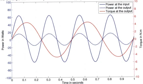
Power and torque results from the dynamical model, for a flapping frequency of 2 Hz and an amplitude of 30 degrees
100l 1 1 1 1 1 110 0u C 201 0 -20- -40- -60- -80--100 -0 6 4 2 0 -2 -4 -6 z EF 0 --8 -10 0.1 0.2 0.3 0.4 0.5 0.6 0.7 0.8 0.9 1 Time in seconds
Figure 2-6: Expected power consumption at the input of the motor (in solid blue) and at the output gear (in dashed blue) as well as the output torque (in red) for an input flapping amplitude of 30 degrees, and at a frequency of 2 Hz.
look like when it is actuating a flapper via a gearbox, at a frequency of 2 Hz and an amplitude of 30 degrees. This plot shows two interesting features:
" The power oscillates at a frequency equal to twice the input frequency " The power becomes negative during a significant portion of its cycle
Those two features are a direct consequence of the presence of silicone around the flapper. Consider the following time intervals that describe the physics of the flapper during one oscillation:
* t E [0; 0.125] sec: The flapper goes from 0' to 30'. As the top silicone is compressed and the bottom one is stretched, the motor needs to provide power. Both the power and the torque are positive. The angular speed of the flapper is null at t = 0.125 sec as it has reached its angular maximum (30'). The torque
also reaches its maximum.
* t E [0.125; 0.25] sec: The flapper goes from 30' to 0'. The stressed silicone
relaxes and provides power to the flapper. The power becomes negative. The system is back at its original position when t = 0.25 sec. The torque is then null and so is the power.
* t E [0.25; 0.5] sec: The flapper goes from 0' to -30' and back to 0'. This second
half-cycle is analogous as the first one except that now, the torque is negative as the flapper is moved towards the negative values of 0. The angular velocity first takes negative values up to 0 = -30' at t = 0.75 sec, then takes positive
values to bring the flapper back to 0 = 0'. The power has the exact same profile
as during the first half-cycle because both the torque and the angular velocity change their signs yet keeping the same behavior in terms of absolute value. The results provide relevant metric for the design of the actuator. A motor is selected so that the nominal power of the motor matches the maximal power required
by the flapper. A gearbox is designed so that it can map the nominal output torque
0
-sFR
FD Ax
p
A,0 x A*
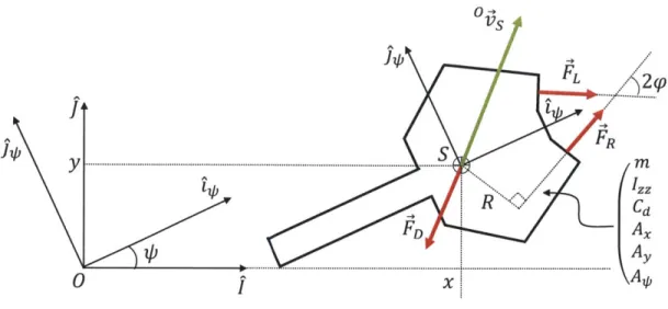
Figure 2-7: Top-view schematic of the model of the robot. Forces are in red, the velocity of the robot is in green.
brought to make sure the bandwidth of the motor is sufficiently large to allow for such high frequency oscillations.
2.4
Trajectory Control
The control of the robot displacements is a primary concern once the robot is built and ready to accomplish missions. The objective is to make sure it can follow a predetermined path at the surface of the water. Keeping the robot at the surface of the water helps reduce the number of degrees of freedom of the robot from six to three (sway, surge and yaw). The control approach for the robot relies on a traditional model-feedback-controller structure. Those three components are derived in the following subsections.
2.4.1
Model
Modelling the robot is a challenging issue since it propels itself by deforming its body in water. The challenge resides in deriving a model that both includes the hydro-elastic behavior of the robot and still stays simple enough to be used on-line, by a micro-controller. As a first approach to solve this problem, a model of
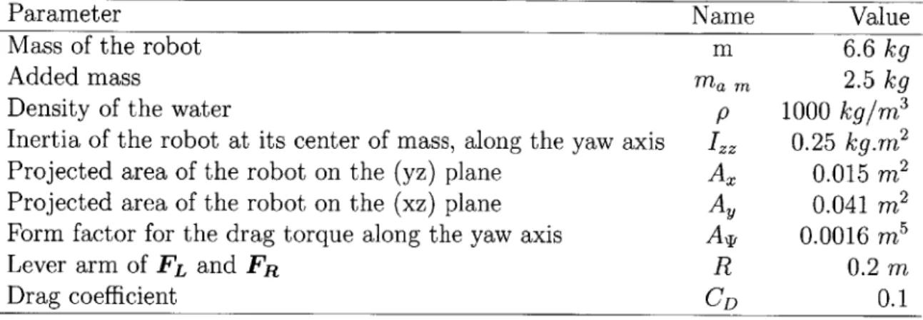
Table 2.2: Values of the parameters used in the model for trajectory control
Parameter Name Value
Mass of the robot m 6.6 kg
Added mass ma m 2.5 kg
Density of the water p 1000 kg/rn3
Inertia of the robot at its center of mass, along the yaw axis IZZ 0.25 kg.m2
Projected area of the robot on the (yz) plane Ax 0.015 m2
Projected area of the robot on the (xz) plane AY 0.041 m2
Form factor for the drag torque along the yaw axis Av 0.0016 m5 Lever arm of FL and FR R 0.2 m
Drag coefficient CD 0.1
the robot is proposed where it is considered as a rigid body. Fig. 2-7 presents a schematic of the model, with the frames, parameters and variables involved. The parameters values are given in the table 2.2. The hydro-elastic interaction between its body and the water is lumped into the two forces produced by the fins: FL for the left fin and FR for the right fin., They are oriented at an angle
4
with respect to the frame(O,
i,,J kx= K). While it is obvious the magnitude varies with the input flapping frequency and flapping amplitude, it is not evident their orientation is dependent on the input. Both the magnitude and orientation of these forces are to be characterized through experimentation. The definition of these forces, using the notations presented in Fig. 2-7 is:FL = FL (Cos t- 4 sin )
FR = FR (cos
#
+ sin#
3The position of the robot is expressed in the ground frame, by the variables x and y. Another frame, attached to the robot, defines the angle T with respect to the ground frame. Using these definitions, the equations of motions can be derived (full derivation in Appendix C):
(m+mam)
(m~mam) =
FL (cos q cOs'
+
sin#
sin T)+
FR (cos#
cos A - sin sin F)pD 2 (Ax Cos T + Ay sin I)
FL (cos#$ sinT - sin# cos T)+ FR (cos#5 sinT+sin# cos T)
P CD 2 (A, sin4T + Ay Cos4')
2
Izz
N
=R ( FR - FL) - CDA 522
(2.5)
Define a state vector: x = [X i y
yX
1 ]T = x2 x3 x4 X5 X6]T , and an inputvector: u = [FL FR]T = [ui U2]T. The equations of motion 2.5 can then be rewritten
under the following form: i = F(x) + G(u)
x 2 cos (x5 -#) m x4 sin (x5 -) m x6 u, + cos (x5 +) m sin(x5 +
#)
U1 + U2 -m P CD 2m P CD 2m X2(Ax cos x5 + AY sin x5) x2
(A. sin x5 + Ay cos x5) x4
R R pCDAq 2
Izz +
Izz
2 Izz(2.6)
Linearizing the equations 2.6 about a fixed point (X0, uo), the system can be
ex-pressed using the conventional state-space representation: 6;i = A 6x
+
B 6u where A and B are the Jacobian matrices of F and G:3:1 = Y2 = Y3 = Y4 = Yi5 = Y6 =
0 1 0 0 0 0 0 1
cos (X50 - #) cos (X5 0 + #)
0 A22 0 0 A25 0 m m
0 0 0 1 0 0 0 0
A= 0 0 0 A44 A4 0 and, B sin (X5 0 -
#)
sin(X50 +)m m 0 0 0 0 0 1 0 0 0 0 0 0 0 A6 6 R R Izz Izz Where: A22 = -CD (A cosx5 0 + AY sin X5 0) x20
A4 4 = CD (Ax sin X50 + AY cos x5 0) X4 0
A6 6 p DA 60
Izz
A25 A25 -sin (X5 0 -
#)
uo -Usin (X5 0 + $) p CD 220 --
(--Ar
sin xso+
Ay cos x5o) 2m m 2m
A4 5 cos (X50 - # + cos (X5 0 +
4)
20 - P CD (A X5 0) 2m m 2 m c A s
These linearized equations can then be used to control the robot using standard tools for control of Linear Time-Invariant (LTI) systems.
2.4.2
Feedback and Controller
The controller chosen to control the robot is a Linear-Quadratic Regulator (LQR) with full state feedback. LQR control is simple to implement on a micro-controller and is well adapted to the state-space formulation of the model of the robot. Moreover,
by essence, LQR control weighs the relative importance of the states and the control
inputs. This allows to easily tailor the response of the controller to make sure the control effort is emphasized towards the more sensitive states. Two limitations subsist to this technique:
" The LQR works on a linear time invariant system. In our case, it means it can only be used to stabilize the robot in the vicinity of the fixed point where the equations of motions are linearized.
" The LQR algorithm needs full state feedback to operate. This means, it needs to know the robot's position, orientation and velocity.
The first limitation is easily tackled by realizing the linearized equations do not depend on the robot's position. They only depend on its orientation, T and its ve-locities x ,
y,
5. Those are set by the value of the fixed point(4
0, uo) the linearizedequations depend on. Therefore, a trajectory consisting of a simple straight line, one joining two waypoints for instance, results in having the states X30, X40, X5o and X60
set to 0 and choosing a forward velocity, x20. The 5 h and 6 th state equations give
that, for this specific trajectory, uio and u20 are equal to a same value, uo . The 2 d
state equation sets the value of uo: uo - p CD AX . The robot can therefore be
4 cos
4
controlled to follow a straight line and have it travel from waypoint to waypoint.
The second limitation is addressed using results developed for strapdown Inertial Navigation Systems (INS). These systems were historically developed to track the position of an aircraft or a missile using only onboard information provided by ac-celerometers, gyroscopes and occasionally, magnetometers. Prior INS were mounted on inertial platforms, mechanically isolated from the various rotations of the body (historically a ship or a submarine). Strapdown INS, on an other hand, are rigidly mounted on the body. They eliminate the mechanical complexity of the platform-based systems, are lighter and cheaper. However they increase the computing com-plexity of the navigation algorithm and require sensors capable of measuring higher angular rates. All of these issues have been resolved thanks to advances in computer technologies and the development of suitable sensors.
The complete derivation for a strapdown INS can be found in [32]. A condensed summary of the key elements is presented hereafter:
Define an Earth-fixed reference frame and a body frame (attached to the robot). The ground velocity v| experienced by the robot and expressed in the Earth frame is given by the following expression:
e = Cb f 2 we x v;+ ge ~ C fb + g,
All upper scripts define the frame in which vectors are expressed in. Here are the
definition of the various terms involved in the equation:
* Cb is the Direction Cosine Matrix relating the two frames.
* fb is the specific force measured by the Inertial Measurement Unit (IMU).
It includes the accelerations due to the motion of the robot with respect to Earth but also the Earth gravity and the Coriolis acceleration due to the Earth rotation.
* 2 ew x ve is the Coriolis acceleration due to the robot moving in a rotating
frame, namely: the Earth. It is highly negligible with respect to the other accelerations and is not implemented in the final algorithm.
* g' is the local gravity vector. It is picked up by the IMU and needs to be accounted for in order to only consider the accelerations that generate motions. This equation can theoretically give updates of ground velocity, and, after inte-gration, give updates of ground position. However, noise, drift, small angular errors between sensors alignments and numerical approximations resulting from a double integration make this algorithm very difficult to implement. It allows to estimate the states of the robot for a few tens of seconds but the estimates will always eventually diverge.
This issue could be addressed by choosing a military grade IMU. The one im-plemented on the prototype is an inexpensive commercial one that can reliably give
orientation estimates but not position ones. The position estimate could also be cor-rected using GPS updates when the robot is swimming at the surface of the water. Finally, if the robot were to be used underwater, a different sensor than an IMU should be used. A Doppler Velocity Log (DVL) is a device that emits several sound waves towards the sea bed and analyses their reflections to determine the robot's velocity vector. It is a widely used system in the world of Autonomous Underwater Vehicles.
Chapter 3
Prototype
3.1
Components and Assembly
3.1.1
Power
Batteries are currently the best solution to provide power to the robot. They are sim-ple, reliable and affordable. The only other alternative would be to harvest energy from the surrounding environment which, in itself, would be a subject of thesis. The Lithium-Polymer (Li-Po) technology is currently offering the highest charge density and it is therefore preferred over other kinds of rechargeable batteries. Three batteries are implemented in the robot, one to power each actuator and a third one to power the electronics. The batteries for the actuators are manufactured by the company Pulse. The Pulse Ultra has 6 cells and delivers 5000 mAh [33]. The battery for the electronics is coming from the distributor Sparkfun [34], has one cell and delivers 2000 mAh, as seen in table 3.1.
A brushless DC motor is preferred among other solutions for the actuation of the
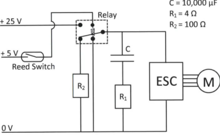
flapper. Reasons that motivate this choice are explained in section 3.2. This choice requires to implement a large capacitor (C) in parallel with each battery (+25V) as depicted in Fig. 3-1. The motor (M) is indeed feeding the power line with energy when it is decelerating. The purpose of the capacitors is to store this energy in order
C = 10,000 pF
R1= 4 (
R2= 100 0
Figure 3-1: Schematic of the electric circuit that delivers the power to the actuator. to prevent over-voltage on the Electronic Speed Controller (ESC). When the circuit is closed, the capacitors demand an inrush of current that has to be accounted for. This motivates the presence of a resistor (R1) in series with each capacitor in order
to limit this current. Another resistor, (R2) helps discharge the capacitor when the
robot is switched off. A relay closes the contacts. Its coil is powered by a third battery which also powers the electronics. This low-voltage battery is connected to the circuit via a reed-switch that acts as a master switch for the robot. When a magnet is approached to the reed-switch, its contact closes, thus connecting the low-voltage battery (+5V) to the electronics and the coils of the two relays. This is how the high power stage is switched on using low power commands.
3.1.2
Sensors
23mm E E 0 LOIE
E r-26 mmIE
E U, (N 26mmFigure 3-2: On the left: GPS the right: Encoder
This subsection presents the sensors that are implemented on the robot for control purposes. Other kinds of sensors (for environmental studies) could be implemented but they are outside the scope of this thesis. In order to control its motion, the robot needs to know its orientation and its position. Two sensors are used for that purpose:
(1) an Inertial Measurement Unit (IMU), the UM6-LT from ChRobotics [35] and (2)
a GPS module, the D2523T from ADH Technology Co. Ltd [36]. Both are presented in Fig. 3-2. The IMU provides measurements of accelerations, angular velocities and magnetic field on all three inertial axes. An Extended Kalman Filter (EKF) coded directly on the IMU provides estimates of the robot's orientation through a serial interface. The GPS provides the latitude and longitude of the robot via a serial interface too. With these two sensors, the robot knows both its orientation and location in space. Finally, two encoders are used to provide feedback on the actuators angular positions. They measure the angular positions of the second to last gear train as there is no space offered on the last train. That slight non-collocation can easily be accounted for in the code by multiplying the measured angle with the gear ratio of the last two gears. Magnetic encoders are preferred to optical ones since magnetic encoders are more robust in humid environments. Optical encoders can provide erroneous measurements if fog builds up on their transparent disk. The chosen magnetic encoders are the MAE3 from USDigital [37]. All these sensors are listed in the table 3.1.
3.1.3
Controllers
54 mm
Figure 3-3: On the left: The Electronic Speed Controller. On the right: the mbed NXP LPC1768
A total of four controllers are used to control the robot. Two Electronic Speed
Controllers (ESC) are needed to operate the two brushless DC motors. They are the equivalent of an H-bridge to a brushed DC motor. They accept a speed command from a higher level controller and make sure the motors follow that command. The ESCs used on the robot are the ESCON 36/3, from Maxon Motor [38].
The higher level control of the robot is achieved by two micro-controllers called mbed NXP LPC1768 [39]. The first mbed is dedicated to provide a reference speed to the ESCs and uses the encoders as feedback. The second mbed determines the robot's behaviour. It provides the first mbed with directions and uses the IMU and GPS for feedback. Fig. 3-3 shows the two controllers.
3.1.4
Communication
Communicating with the robot is crucial to make sure the mission is going as planned. It is also a useful tool to control the robot at a distance. To that purpose, a radio module needs to be able to interface easily with the micro-controller. The Xbee modules from Digi International [40] are off-the-shelf transceivers that convert serial data (RS-232) into radio waves, eliminating the hassle of developing a radio module for the robot. Every module have the same small footprint, allowing to swap modules to meet the frequency regulations of the country the robot is operated in. Details on the module used in the robot can be found in the table 3.1.
3.1.5
Housing
All components are mounted inside a container called the shell of the robot. Since the
size of the robot is determined by the size of the mold, the shell needs to reproduce the shape of the mold in order to maximize the available space. Therefore, the shell is designed to leave a consistent spacing between its surface and the surface of the mold. This space is filled with silicone during the casting process and forms the skin of the robot.
overall resulting shape is too intricate for standard machining techniques but is very easy to reproduce using a 3D printer. The shell is therefore printed, in three parts, that are later assembled to form one rigid shell. Fig. 3-4 presents one part of the shell as it is when taken out of the printer. This figure also presents the other parts of the shell. Fig. 3-5 shows the open shell once all the components have been mounted on it. Fig. 3-6 is an exploded view of the assembly of the robot and its components.
Table 3.1: Design table
Disk length 0.6 m
Length with tail 1.25 m
Dimensions
Mass of the robot 6.6 kg
Volume of the robot 6.6 L Actuator battery voltage 22.2 V Actuator battery capacity 4.5 A.h Electrical Electronics battery voltage 3.7 V
Electronics battery capacity 2 A.h Motor nominal power 70 W
ESC ESCON 36/3 [38]
Control Robot controllers mbed [39]
IMU UM6-LT by ChRobotics [35]
& Sensing GPS D2523T by ADH Technology [36]
Encoder MAE3 from USDigital [37]
Device Xbee-pro 868 from Digi Int. [40] Communication Range in air 500 m
Figure 3-4: On the left: center part of the shell as it is out of the 3D printer. On the right: the three parts of shell
1. Soft silicone body 2. Soft silicone tail
3. Tail fixture cast in #2
4. Anchor Point for the tail on #9
5. Nose
6. Actuation subassemblies
7. Shell 1 contains the actuation 8. Shell 2 contains the batteries 9. Shell 3 contains the ESCs, #15 10. Cover 1 supports the electronics 11. Cover 2
12. Cover 3
13. Communication module Xbee
14. Micro-controllers Mbed
15. Electronic Speed Controllers 16. Capacitors for the motors 17. LiPo batteries, 6 cells, 4.5 Ah 18. LiPo battery, 1 cell, 2 Ah
00
(D -q~
D
CJ)O
3.2
Actuation
The motor is selected so that its nominal power matches the maximum theoretical power at the maximum operating frequency and amplitude. That is, Pm, = 65 W for a flapping frequency of 2 Hz and a flapping amplitude of 30'. Specifically, the motor used in the latest prototype is the EC-45 flat, from Maxon Motor [41], and is rated at 70W. It is a brushless DC motor, a technology that provides motors with high power densities and virtually no maintenance.
The motor needs a gearbox to transform its high angular velocity into useful torque. That purpose is usually fulfilled by a gearbox; a standard device that is avail-able from the same manufacturer as the motor. However, no off-the-shelf solution meets both the space and torque requirements. An original gearbox was therefore designed, machined and assembled.
O.Oeratin. Ran.e
n [rpm] Continuous operation
In observation of above listed thermal resistance
70 W (lines 17 and 18) the maximum permissible winding
10000 temperature will be reached during continuous
operation at 250C ambient.
0 Thermal limit
Short term operation
4000 The motor may be briefly overloaded (recurring).
2000
"'""""-'""" Assigned power rating
25 50) 75 10 125 150 M [mNm]
0 2.0 3.0 4.0 IJAI
Figure 3-7: Capabilities of the motor in terms of torque and angular velocity Since the motor is selected based on the power it delivers at a flapping regime of
30 degrees of amplitude and 2 Hz, the gearbox is designed to operate at this regime
too. Fig. 3-7 presents the characteristic plot of the motor capabilities in terms of torque and angular velocities. This plot provides the nominal value of the angular velocity of the motor: Wnom,motor = 4820 rpm. It also provides the nominal value of