HAL Id: tel-01314133
https://tel.archives-ouvertes.fr/tel-01314133
Submitted on 10 May 2016HAL is a multi-disciplinary open access archive for the deposit and dissemination of sci-entific research documents, whether they are pub-lished or not. The documents may come from teaching and research institutions in France or abroad, or from public or private research centers.
L’archive ouverte pluridisciplinaire HAL, est destinée au dépôt et à la diffusion de documents scientifiques de niveau recherche, publiés ou non, émanant des établissements d’enseignement et de recherche français ou étrangers, des laboratoires publics ou privés.
Fabien Defrance
To cite this version:
Fabien Defrance. Instrumentation of a 2.6 THz heterodyne receiver. Instrumentation and Methods for Astrophysic [astro-ph.IM]. Université Pierre et Marie Curie - Paris VI, 2015. English. �NNT : 2015PA066521�. �tel-01314133�
T
HÈSE DE DOCTORAT
Spécialité : Méthodes Instrumentales en Astrophysique et leurs Applications Spatiales
Présentée par
Fabien DEFRANCE
Pour l’obtention du grade de docteur de l’université Pierre et Marie Curie
Instrumentation d’un récepteur hétérodyne à
2.6 THz
Thèse soutenue le 14 décembre 2015 devant un jury composé de :
M. Aziz BENLARBI-DELAÏ
L2E
Président du jury
M. Paul CROZAT
IEF
Rapporteur
M. Alessandro NAVARRINI
INAF
Rapporteur
Mme. Martina WIEDNER
LERMA
Directrice de thèse
M. Massimiliano CASALETTI
L2E
Examinateur
Mme. Christine LETROU
Télécom SudParis
Examinatrice
M. Julien SARRAZIN
L2E
Invité
Thèse préparée à l’Observatoire de Paris, au Laboratoire d’Études du Rayonnement de la
Matière en Astrophysique et Atmosphères (LERMA)
Les observations astronomiques nous permettent d’étudier l’univers et de comprendre les phénomènes qui le gouvernent. La matière visible dans l’univers émet des ondes à des fréquences très diverses, réparties sur tout le spectre électromagnétique (domaines radio, submillimétrique, infrarouge, visible, ultraviolet, X et gamma). Ces ondes nous renseignent sur certaines caractéristiques physico-chimiques des éléments observés (nature, tempéra-ture, mouvement, etc.). Des télescopes couvrant différentes plages de fréquences sont néces-saires pour observer l’ensemble du spectre électromagnétique. Les radio-télescopes, sensi-bles aux ondes (sub)millimétriques, sont principalement dédiés à l’observation de la matière froide présente dans le milieu interstellaire. Le milieu interstellaire est le berceau des étoiles et son étude est essentielle pour comprendre les différentes étapes de la vie des étoiles. La fréquence maximale d’observation des radio-télescopes est en augmentation depuis la fabrication des premiers télescopes dans les années 1930. Récemment, des radio-télescopes capables de détecter des signaux dans l’infrarouge lointain, au delà de 1 THz, ont été développés. Ces avancées technologiques ont été motivées, entre autres, par la présence, dans le milieu interstellaire, de molécules et d’ions uniquement observables à des fréquences supérieures à 1 THz. Pour observer des raies avec une haute résolution spectrale, les radio-télescopes sont équipés de récepteurs hétérodynes. Ce type de récepteur permet d’abaisser la fréquence de la raie spectrale observée tout en conservant ses caractéristiques (une raie observée à 1 THz peut, par exemple, être décalée à une fréquence de 1 GHz). Cette tech-nique permet d’observer des raies avec une très haute résolution spectrale et c’est pourquoi les récepteurs hétérodynes sont largement utilisés pour les observations de raies spectrales aux fréquences GHz et THz. Dans les récepteurs hétérodynes, un oscillateur local (OL) émet un signal monochromatique à une fréquence très proche de celle du signal observé. Les deux signaux sont superposés à l’aide d’un diplexeur et transmis à un mélangeur. Ce dernier réalise le battement des deux signaux et génère un signal identique au signal observé mais à une fréquence plus faible.
Durant ma thèse, j’ai travaillé sur la construction, la caractérisation et l’amélioration d’un récepteur hétérodyne à 2.6 THz. Cette fréquence d’observation (2.6 THz) est l’une des plus hautes atteintes par les récepteurs hétérodynes THz existant actuellement, ce qui constitue un défi technologique très important. Dans le but de caractériser et d’améliorer ce récepteur, je me suis concentré sur trois aspects essentiels :
1. La stabilité : C’est l’une des caractéristiques principales des récepteurs hétérodynes. Elle est liée au bruit généré par le récepteur et détermine le temps pendant lequel le récepteur peut intégrer le signal reçu sans avoir besoin d’être recalibré. Meilleure est la stabilité du récepteur, plus longtemps il peut intégrer le signal observé et plus le
bruit de la mesure est atténué. La stabilité d’un récepteur peut être caractérisée par la variance d’Allan. Dans ma thèse, je distingue les variances d’Allan totale et spec-trale. La variance d’Allan totale permet d’estimer la stabilité en puissance du récepteur sur l’ensemble de sa bande passante. La variance d’Allan spectrale donne une estima-tion de la stabilité de la forme du spectre (on considère la variaestima-tion des canaux de fréquences les uns par rapport aux autres). À l’aide de ces deux types de variances d’Allan, j’ai pu calculer la stabilité de notre récepteur et conclure qu’avec notre os-cillateur local à 600 GHz elle est comparable à celle d’autres récepteurs hétérodynes internationaux comme GREAT et HIFI. En mesurant la stabilité des différents éléments du récepteur, j’ai pu en déduire que l’oscillateur local à 1.4 THz et l’alimentation de notre mélangeur étaient les principales sources d’instabilités.
2. Le diplexeur : Cet élément permet de coupler le signal observé avec celui de l’oscillateur local (OL). Le but du diplexeur est de transmettre le maximum de puissance du sig-nal observé et suffisamment de puissance de l’OL pour permettre un fonctionnement optimal du mélangeur. Le diplexeur le plus couramment utilisé aux fréquences THz est un film semi-réfléchissant en Mylar®. Il transmet généralement environ 90 % du signal observé et réfléchit environ 10 % du signal de l’OL. À des fréquences inférieures à 1 THz, les OL émettent assez de puissance pour que 10 % suffisent au fonction-nement du mélangeur. Pour notre récepteur à 2.6 THz, cette méthode n’est pas en-visageable car les OL standards n’émettent pas assez de puissance. J’ai donc conçu, testé et amélioré un autre type de diplexeur, un interféromètre de Martin-Puplett. Cet interféromètre utilisant deux grilles polarisantes, deux miroirs en toit et un miroir el-lipsoïdal pour focaliser le signal de l’OL, peut théoriquement transmettre à la fois le signal observé et celui de l’OL avec très peu de pertes. J’ai donc conçu et caractérisé les différents éléments de l’interféromètre avant de les assembler et de mesurer l’efficacité globale de l’interféromètre. Cela m’a permis d’obtenir une transmission de 76 % du signal de l’OL et d’estimer la transmission du signal observé à 79 % environ. Cet inter-féromètre est donc opérationnel pour être utilisé dans notre récepteur hétérodyne à 2.6 THz. De plus, les mesures des différents éléments de l’interféromètre m’ont permis de déterminer quels éléments généraient le plus de pertes. Ainsi, le remplacement des grilles polarisantes devrait permettre une amélioration de l’efficacité de notre inter-féromètre de Martin-Puplett à 2.6 THz.
3. Le réseau de phase : Il est utilisé pour diviser le faisceau de l’OL en plusieurs faisceaux et permettre la fabrication de récepteurs hétérodynes à plusieurs pixels. Les récepteurs hétérodynes ne comportent généralement qu’un seul pixel. Pour augmenter le nombre de pixels, il est nécessaire d’utiliser plusieurs mélangeurs qui doivent, chacun, recevoir un signal de l’OL couplé avec une partie du signal observé. Pour permettre la création d’un récepteur hétérodyne multi-pixel, j’ai conçu et testé un nouveau type de réseau de
phase, que nous avons appelé Réseau de phase global, permettant de diviser le faisceau de l’OL en plusieurs faisceaux. J’ai développé un programme numérique pour calculer des profils de réseaux de phase permettant de générer le nombre souhaité de faisceaux avec une excellente efficacité. Les profils de phase générés par ce programme n’ont pas de contrainte géométrique, à la différence des réseaux de phase actuellement utilisés aux fréquences THz, les réseaux de Dammann qui ont une géométrie discrète, et les réseaux de Fourier qui ont une géométrie continue. Les Réseaux de phase globaux que j’ai développés peuvent être non-périodiques et pourraient également avoir d’autres applications, comme modifier la forme d’un faisceau. J’ai réalisé deux prototypes de Réseaux de phase globaux divisant le faisceau de l’OL en quatre faisceaux et fonction-nant à 600 GHz. Les deux prototypes sont basés sur le même design, mais l’un fonc-tionne en transmission (il est en TPX®, un plastique assez transparent à 600 GHz), et l’autre, en laiton, fonctionne en réflexion. J’ai pu vérifier et améliorer l’efficacité théorique de ces prototypes avec FEKO, un logiciel de simulation électromagnétique. Les deux prototypes ont été réalisés par une société extérieure et testés dans notre laboratoire à 600 GHz. J’ai mesuré une efficacité de 76± 2 % pour le prototype en réflexion, et 62± 2 % pour le prototype en transmission. Ces valeurs sont très bonnes et la correction d’une erreur d’usinage sur le réseau en transmission devrait encore augmenter son efficacité. L’efficacité de ces prototypes de Réseaux de phase globaux est parmi les meilleures au monde pour les fréquences THz, et de prochains prototypes à 1.4 THz et 2.6 THz sont prévus.
Finalement, le travail accompli durant cette thèse de doctorat constitue une étape impor-tante vers la réalisation d’un récepteur hétérodyne multi-pixel à 2.6 THz utilisant un in-terféromètre de Martin-Puplett comme diplexeur, et possédant de très bonnes caractéris-tiques de stabilité et de sensibilité. Ce futur récepteur hétérodyne pourrait être utilisé dans d’importants projets internationaux comme CIDRE, Millimetron, CCAT, GUSSTO ou THEO.
Mots clés : Récepteur hétérodyne, térahertz, THz, Martin-puplett, variance d’Allan, réseau de phase, stabilité, multi-pixel, oscillateur local, diplexeur, optique gaussienne, quasiop-tique, réseau de Dammann.
(Sub)Millimeter-telescopes are often used to observe the interstellar medium in the uni-verse and they enable us to study the stellar life cycle. To detect and study some important molecules and ions, we need receivers able to observe at frequencies above 1 THz. Re-ceivers working at such high frequencies are quite new and the 2.6 THz heterodyne receiver I built and characterized during my PhD represents the state-of-the-art of THz heterodyne receivers. I especially focused on three important aspects of this receiver: its stability, the superimposition of the local oscillator signal (LO) and the observed signal by a diplexer, and the splitting of the LO signal by a phase grating. The stability was calculated with the Allan variance and I found that the two elements limiting the stability of our receiver were the 1.4 THz local oscillator and the mixer bias supply. The Martin-Puplett interferometer (MPI) diplexer I designed, built and tested is able to transmit 76 % of the LO power at 2.6 THz and we estimate a transmittance around 79 % for the observed signal. This MPI is operational and ready for the next generation of heterodyne receivers. Splitting the LO signal is essen-tial to build heterodyne receivers with several pixels, which allows us to get spectra of the universe at many positions in the sky simultaneously. I have developed a new kind of grat-ing, called Global gratings, and I made two prototypes of these Global phase gratings able to split the LO beam into four beams. These two phase grating prototypes, a transmissive and a reflective one, were optimized for 610 GHz and showed, respectively, an efficiency of 62± 2 % and 76 ± 2 %. These excellent results validate the design and fabrication processes of this new kind of grating. In conclusion, the work accomplished during this PhD consti-tutes an important step toward the realization of a very stable and highly sensitive 2.6 THz multi-pixel heterodyne receiver using a MPI diplexer.
Key words: Heterodyne receiver, THz, Martin-Puplett, Allan variance, phase grating, stabil-ity, multi-pixel, local oscillator, diplexer, Gaussian optics, quasioptics, Dammann grating.
Je tiens à remercier Martina Wiedner, ma directrice thèse, pour son aide et son soutien tout au long de cette thèse, ainsi que pour ses qualités humaines et scientifiques. Je lui suis très reconnaissant de la grande liberté qu’elle m’a laissé durant ces trois années, ainsi que de l’opportunité qu’elle m’a donné de participer à des conférences aux Pays-Bas, en Russie et aux Etats-Unis, ainsi qu’à une semaine d’observation au 30m de l’IRAM. Je tiens aussi à remercier Paul Crozat et Alessandro Navarrini qui ont accepté d’être les rapporteurs pour ma soutenance de thèse, et dont les commentaires m’ont été très précieux. Je remercie également Aziz Benlarbi-Delaï, Martina Wiedner, Massimiliano Casaletti, Christine Letrou et Julien Sarrazin pour avoir accepté de faire partie du jury. Je remercie aussi l’ensemble des personnes du LERMA pour leur accueil chaleureux, en particulier l’équipe du bâtiment Lallemand qui m’a aidé et supporté durant ces trois années. Merci à Grégory Gay, pour sa disponibilité, son aide précieuse, sa bonne humeur, mais aussi pour ses goûts musicaux qu’il m’a fait partager et pour certaines expériences à base d’azote liquide. Merci à Yan Delorme pour ses nombreux conseils et son soutien, à Alexandre Ferret pour l’esprit de travail si par-ticulier que nous avons réussi à développer dans notre bureau, à Michèle Batrung pour son soutien culinaire, à Maurice Gheudin pour ses idées et ses coups de main, à Jean-Michel Krieg pour sa confiance. Je remercie également les nouveaux arrivants, Anastasia Penkina, Duccio Delfini et François Joint, d’avoir contribué à la création du bureau des doctorants, as-surément la plus belle pièce du bâtiment Lallemand. Je remercie également Thibault Vacelet et Roland Lefèvre, dont les compétences en micro-imagerie m’ont été très utiles, ainsi que Faouzi Boussaha, Christine Chaumon et Alain Maestrini pour leurs conseils et les moments passés ensemble lors de conférences. Je tiens aussi à remercier Die Wang pour m’avoir per-mis de ne pas trop perdre mon chinois et pour son poulet au coca, Jordane Mathieu pour son gateau de l’amitié qui faisait beaucoup de bulles, ainsi que Shanna Li pour son atelier de ravi-olis chinois. Je tiens à remercier Laurent Pelay et les personnes de l’atelier de mécanique qui m’ont été d’une aide précieuse durant toute la durée de la thèse pour réaliser divers éléments mécaniques et optiques. Je remercie également toutes les autres personnes de l’Observatoire que j’ai côtoyées et qu’il serait trop long de citer. Je tiens à remercier l’équipe du L2E à l’UPMC qui m’a accueilli, et plus particulièrement Julien Sarrazin et Massimiliano Casaletti dont les conseils m’ont été très précieux pour développer des réseaux des phase. Je n’oublie pas non plus toute l’équipe d’Astro-jeunes, dont la réussite tient très certainement à sa grande proportion d’auvergnats, avec qui j’ai participé au festival d’astronomie de Fleurance. Merci à vous Nicolas Laporte, Simon Nicolas, Aurélia Bouchez, Laurianne Palin, Gabriel Foenard, Ilane Schroetter, Philippe Peille, Vincent Heussaff, David Quénard, William Rapin, Nicolas Vilchez, Arnaud Beth, Claire Divoy et Jason Champion. Je remercie aussi Thierry Duhagon
pour son investissement dans le festival, ainsi que Julie Gourdet sans qui je n’en aurais ja-mais eu connaissance. Je remercie aussi le CNES qui à financé ma thèse, et Gilles Cibiel mon responsable au CNES. Je suis également reconnaissant à Pierre Martin-Cochet et Paul Ho, de l’ASIAA, dont le rôle a été déterminant dans l’obtention de cette thèse. Je remercie aussi Hugh Gibson pour m’avoir beaucoup aidé dans mes simulations électromagnétiques et pour m’avoir fait découvrir qu’il pouvait exister du bon cheddar. Merci à Serena Wong pour son soutien et ses mails à rallonge qui pourraient remplir plusieurs thèses, et merci à Edwige Chapillon pour m’avoir fait découvrir Grenoble depuis les airs. Finalement, je tiens tout particulièrement à remercier mes parents qui m’ont toujours soutenu et encouragé, et qui m’avaient offert, il y a maintenant plus de vingt ans, un livre sur le système solaire. Encore merci. Enfin, je pense à toi mon Schtroumpf qui commence ta thèse, bon courage!
Résumé ii Abstract v Acknowledgements vi Contents viii Abbreviations xi 1 Introduction 1
2 Terahertz heterodyne receivers 4
2.1 Motivation . . . 4
2.2 THz heterodyne receivers in astronomy . . . 4
2.2.1 Main characteristics of heterodyne receivers . . . 4
2.2.2 Overview of existing THz heterodyne receivers . . . 5
2.3 General principle of heterodyne receivers . . . 6
2.3.1 The heterodyne principle. . . 6
2.3.2 Sensitivity of heterodyne receivers . . . 8
2.4 Description of the different elements of a THz heterodyne receiver. . . 11
2.4.1 The mixer . . . 11
2.4.2 The local oscillator. . . 14
2.4.3 The diplexer. . . 17
2.4.4 The IF chain and the spectrometer . . . 18
2.5 Our 2.6 THz heterodyne receiver . . . 19
2.5.1 Description of our 2.6 THz heterodyne receiver . . . 19
2.5.2 Main aspects of this PhD . . . 21
3 Stability of the heterodyne receiver 22 3.1 Introduction . . . 22
3.1.1 Motivation. . . 22
3.1.2 Influence of the noise on the optimal integration time . . . 23
3.2 The Allan variance . . . 25
3.2.1 Background and theory . . . 25
3.2.3 Total power and spectral Allan variance. . . 28
3.2.4 The calculation algorithm . . . 29
3.3 Stability of our heterodyne receiver . . . 30
3.3.1 Warm intermediate frequency chain and DFTS . . . 30
3.3.2 Stability of the bias circuit and the cryogenic amplifier . . . 35
3.3.3 Stability of the local oscillator and the HEB mixer . . . 37
3.4 Conclusion . . . 41
4 The Martin Puplett Interferometer (MPI) 43 4.1 Motivation . . . 43
4.2 Gaussian beam optics. . . 44
4.2.1 Context and motivation. . . 44
4.2.2 Electric field distribution of a Gaussian beam . . . 45
4.2.3 Gaussian beam characteristics. . . 46
4.2.4 Conclusion. . . 49
4.3 Description of the MPI . . . 50
4.3.1 Input of the MPI . . . 50
4.3.2 Detailed description of the elements of the MPI . . . 51
4.3.3 The rotation of the polarization in the MPI . . . 53
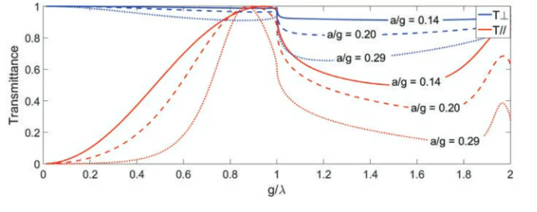
4.3.4 The bandwidth of the MPI . . . 53
4.4 Design of our MPI . . . 55
4.4.1 Calculation of the ellipsoidal mirror (MLO) . . . 55
4.4.2 Calculation of the grids’ required characteristics. . . 58
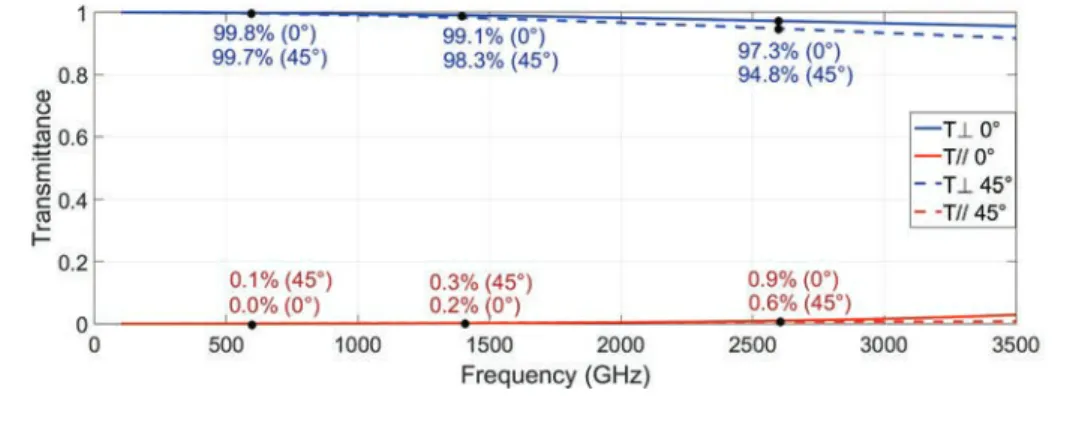
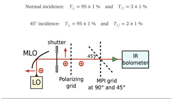
4.5 Test and evaluation of each individual component of the MPI . . . 62
4.5.1 The ellipsoidal mirror (MLO) . . . 62
4.5.2 The polarizing grids . . . 63
4.5.3 Efficiency of the roof-top mirrors . . . 67
4.5.4 Air absorbance . . . 67
4.6 Efficiency of the whole MPI . . . 70
4.6.1 Presentation of the experiment . . . 70
4.6.2 Different steps of the experiment . . . 71
4.6.3 Conclusion. . . 74
4.7 Conclusion . . . 75
5 Phase gratings 76 5.1 Background and theory . . . 76
5.1.1 Motivation. . . 76
5.1.2 Presentation of the phase gratings . . . 77
5.2 The stepped phase gratings . . . 77
5.2.1 Overview of the stepped phase gratings. . . 77
5.2.2 Theory of Dammann gratings . . . 79
5.2.3 Test of a transmissive Dammann grating . . . 80
5.3 The Fourier grating . . . 84
5.4 The Global phase grating . . . 85
5.4.1 General presentation . . . 85
5.4.2 Numerical calculation. . . 85
5.4.4 Electromagnetic simulations . . . 92
5.5 Reflective and transmissive phase grating prototypes . . . 93
5.5.1 Design considerations for the two prototypes . . . 93
5.5.2 Numerical calculation. . . 94
5.5.3 Design of the transmissive and reflective phase gratings . . . 95
5.5.4 Electromagnetic simulations . . . 96
5.5.5 Mechanical design . . . 102
5.5.6 Geometrical measurements of the 2 prototypes . . . 103
5.5.7 Electromagnetic simulation of the manufactured reflective grating 105 5.5.8 Test of the 2 prototypes. . . 107
5.5.9 Noise temperature measurement of the receiver with a phase grating 111 5.6 Conclusion . . . 112
6 Conclusion 114 A Gaussian beam optics 117 A.1 Theory of the Gaussian beam optics . . . 117
A.1.1 The wave equation. . . 117
A.1.2 The Helmholtz equation . . . 118
A.1.3 The paraxial wave equation . . . 118
A.1.4 The fundamental Gaussian mode equation . . . 119
A.1.5 Expression of the beam parameter . . . 120
A.1.6 The radius of curvature and the beam radius. . . 121
A.1.7 The phase shift factor . . . 121
A.1.8 Final expression of the fundamental Gaussian mode . . . 122
A.1.9 Electric field distribution of a Gaussian beam . . . 122
A.2 Gaussian beam characteristics . . . 122
B Functioning of the Martin Puplett interferometer 124 B.1 Rotation of the polarization of the RF signal in the MPI. . . 124
B.2 Bandwidth of the MPI . . . 126
B.3 Water vapor absorption . . . 128
C Theory of the Dammann grating 131 C.1 Approximation of the Maxwell’s equations. . . 131
C.2 Detail of the phase modulation generated by the Dammann grating . . . . 132
C.3 Example of a 1x2 Dammann grating . . . 135
Technical terms
2SB Two Side Bands
CAD Computer Aided Design
DFTS Digital Fourier Transform Spectrometer
DG Dammann Grating
DSB Double Side Band FFT Fast Fourier Transform HDPE High Density Polyethylene HEB Hot Electron Bolometer
HRFZ Si High Resistivity Float Zone Silicon IF Intermediate Frequency
ISM Interstellar medium LO Local Oscillator LSB Lower Side Band
MPI Martin-Puplett Interferometer QCL Quantum Cascade Laser
RF Radio Frequency
SEM Scanning Electron Microscope SSB Single Side Band
USB Upper Side Band
Laboratories
IRAM Institut de RadioAstronomie Millimetrique
LERMA Laboratory for Studies of Radiation and Matter in Astrophysics LPN Laboratory of Photonics and Nanostructures
MPQ Materials and Quantum Phenomena
Telescopes and instruments
ALMA Atacama Large Millimeter/sub-millimeter Array APEX Atacama Pathfinder Experiment
CCAT Cerro Chajnantor Atacama Telescope CHAMP Carbon Heterodyne Array of the MPIfR
CIDRE Deuterium Identification Campaign by hEterodyne Reception COBE Cosmic Background Explorer
CONDOR CO N+ Deuterium Observations Receiver EMIR Eight MIxer Receiver
GREAT German REceiver for Astronomy at Terahertz frequencies GUSSTO Galactic/Xgalactic Ultra long duration balloon
Spectroscopic Stratospheric THz Observatory HHT Heinrich Hertz Telescope
HIFI Heterodyne Instrument for the Far-Infrared KAO Kuiper Airborne Observatory
KOSMA Koelner Observatorium fuer SubMillimeter Astronomie MPIfR Max Planck Institute for Radio Astronomy
NOEMA NOrthern Extended Millimeter Array RLT Receiver Lab Telescope
SMART Sub-Millimeter Array Receiver for Two frequencies SOFIA Stratospheric Observatory for Infrared Astronomy Desert STAR Submillimeter Telescope Array Receiver
STO Stratospheric THz Observatory THEO Terahertz Heterodyne Observatory upGREAT Extension of GREAT receiver
Introduction
Nearly all astronomical observations rely on electromagnetic waves. Our knowledge of the Universe has long been based on optical observations. However, since the last century, enor-mous technological advances enabled us to observe nearly the whole frequency spectrum. The emergence of radio transmissions led to the development of astronomical receivers for radio and sub-millimeter waves. At these frequencies, we are especially sensitive to the emis-sion of cold matter, principally located in the interstellar medium (ISM). The ISM contains molecular clouds where stars and planetary systems are created. Therefore, radio and sub-millimeter astronomical receivers are essential to understand the stellar life cycle. They also allow us to study the composition of molecular clouds in the Universe. Until now, technolog-ical progress continuously increased the maximum observation frequency of sub-millimeter receivers. Very recently, the first receivers above 1 THz have been built. Such receivers are used to explore the far-infrared gap which is the frequency range located between infrared and THz frequencies (figure1.1). This frequency range has, so far, been little observed by astronomers and it is one of the last parts of the spectrum remaining mostly unexplored.
As shown on figure1.1, far infrared radiation is mostly absorbed by the Earth atmosphere, due to the presence of water vapor. Thus, all receivers observing at frequencies above 1 THz must operate from very high altitudes (high mountain, plane, stratospheric balloon or satel-lite).
Two kinds of receivers exist at THz frequencies. Bolometers, which measure the total power received over a large frequency range; and heterodyne receivers, which can generally achieve a very high spectral resolution and are especially used for spectral line observations. At millimeter and sub-millimeter wavelengths, it is possible to detect rotational or vibrational lines of many molecules, as well as fine structure lines of ions. The observation of molecular transitions allows us to determine many physical and chemical characteristics of molecular clouds. The THz spectrum, which remains partly unexplored, contains a few very important lines not observable at lower frequencies (except for OH): N+ (1.46 THz), C+ (1.90 THz), OH (2.51 THz), HD (2.68 THz) and OI (4.75 THz).
• The fine structure line of N+at 1.46 THz is the third strongest cooling line in our galaxy, as observed by the telescope COBE. N+ is a marker of the warm ionized medium.
• C+has also been observed by COBE. It is the strongest line of our galaxy and the most important ISM cooling line in the frequency range of COBE. C+is seen in all the phases of the ISM: the ionized medium, the cold neutral medium and the moderately dense molecular medium.
• Deuterium is one of the primordial elements which has been exclusively created in the Big Bang. In the universe, the D/H (deuterium/hydrogen) ratio decreases, as deuterium is burned by stars but never created. Thus, the D/H ratio is a measure of the history of star formation since the creation of the Universe. Measurements of HD can be used to calculate the D/H ratio, or if the ratio is known, HD can be used as a tracer for H2.
• The OH molecule is a fundamental tracer for the understanding of the oxygen chem-istry and the formation of water. The abundance of OH is linked to that of H2O and
O2 in the ISM. Thus, OH observations are essential to study the numerous aspects of the interstellar chemistry for oxygen and water.
• Neutral atomic oxygen OI can be used to trace diffuse molecular gas and it is also a major coolant of the dense interstellar medium. Moreover, it is used to study the
physical conditions in the photo-dissociation regions (PDR) around massive young stars.
Therefore, the interest in observing these spectral lines motivates the development of het-erodyne receivers above 1 THz.
This PhD thesis was initially dedicated to the CIDRE project, a heterodyne receiver whose goal was to observe HD and OH at 2.68 THz and 2.74 THz. As these frequencies are mostly absorbed by the atmosphere, CIDRE was planned to be carried by a stratospheric balloon, to observe the interstellar medium from an altitude of 40 km. The CIDRE project was sus-pended for budget reasons in 2014. However, this PhD remained dedicated to the devel-opment and improvement of a 2.6 THz multi-pixel prototype heterodyne receiver, because similar receivers will be required for future radio-telescope projects, like Millimetron [1], CCAT [2] and GUSSTO. A satellite project named THEO (THz heterodyne observatory) has been recently proposed by Gerin and Wiedner (Paris Observatory, LERMA). The target lines of this instrument are C+, N+ and OI, and its development will directly benefit from this PhD work. The development of a heterodyne receiver at such high frequencies is technically very challenging.
During my PhD, I developed, built and characterized a 2.6 THz prototype receiver that rep-resents the state-of-art of THz heterodyne receivers. In particular, I studied three aspects of my prototype heterodyne receiver:
1. The stability of the receiver and its components.
2. The optics, by designing, building and testing a Martin Puplett interferometer.
3. The distribution of the local oscillator beam, for which I designed and tested two phase grating prototypes.
The next chapter (chapter2) starts with an introduction of heterodyne receivers, followed by a complete description of our 2.6 THz receiver and a detailed presentation of the other chapters of this thesis. Then, the three main subjects of my thesis, listed above, are developed in detail in chapters3,4and5. Each of these chapters focuses on a specific aspect of our 2.6 THz heterodyne receiver. Finally, this thesis finishes with a conclusion of my work in chapter6.
Terahertz heterodyne receivers
2.1
Motivation
Heterodyne receivers have revolutionized radio astronomy and receivers for higher and higher frequencies have been built. Recently the first heterodyne receivers above 1 THz have been built and tested. For my thesis, I have built characterized and improved a proto-type receiver at 2.6 THz for the next generation of space-borne telescopes.
This chapter provides the reader with background information concerning THz heterodyne receivers, useful to understand the other chapters of this thesis. This chapter is divided into different parts. It starts with a brief description of existing heterodyne receivers above 1 THz. Then, I describe the functioning and main characteristics of standard heterodyne receivers, and I detail the different elements constituting THz heterodyne receivers. Finally, the last part of this chapter contains a complete description of our 2.6 THz heterodyne receiver, and a presentation of the different aspects of my thesis.
2.2
THz heterodyne receivers in astronomy
2.2.1
Main characteristics of heterodyne receivers
Heterodyne receivers are an essential part of radio-astronomy and have lead to a wealth of discoveries. In contrast to bolometers, they usually have a very high spectral resolution
and are ideally suited to observe line emissions, from which we can deduce the physical and chemical conditions of the interstellar medium.
2.2.2
Overview of existing THz heterodyne receivers
Several THz heterodyne receivers operating above 1 THz are already working on ground based and space based telescopes, some of them are listed below and are shown in figure2.1. They are all using HEB mixers (cf. section2.4.1), except the first one, KAO’s receiver, which was using a Schottky diode mixer, less sensitive but covering a larger bandwidth than HEBs.
• The Kuiper Airborne Observatory (KAO) started observing in 1975 and it has been operating during 20 years, before being replaced by SOFIA. It was carrying a 91 cm diameter primary reflector and was operating from a plane. The heterodyne receiver of KAO was able to observe from 700 GHz to 3 THz (cf. Röser [3]).
• The Receiver Lab Telescope (RLT) has been intermittently operating since 2002 from an altitude of 5525 meters, on Cerro Sairecabur, in Chile. It has been the first ground based telescope to observe at frequencies above 1 THz (cf. Marrone et al. [4]).
• CONDOR (CO N+ Deuterium Observations Receiver) was the first ground based het-erodyne receiver to be tested on a large telescope, the APEX 12m telescope, in 2006. It observed at frequencies between 1.25 THz and 1.53 THz [5][6]. The APEX telescope is also located in the Chilean Andes (Llano de Chajnantor) at an altitude of 5105 meters.
• The HIFI (Heterodyne Instrument for the Far-Infrared) instrument of Herschel satellite started observing in early 2010, from space [7][8][9]. It covers frequency ranges between 488 GHz and 1272 GHz, and between 1430 GHz and 1902 GHz.
• The GREAT (German REceiver for Astronomy at Terahertz frequencies) [10] and up-GREAT [11] instruments are two heterodyne receivers which have been operating on SOFIA airplane observatory [12], since 2012 and 2015 respectively. These two het-erodyne receivers cover different frequency windows between 1.25 THz and 4.7 THz.
• The Stratospheric THz Observatory (STO) [13] has an heterodyne receiver embedded below a stratospheric balloon which can observe from an altitude of 38 km. A new version of this balloon, STO-2 [14] will be launched in late 2015 and will be able to observe three frequency bands centered on 1.4 THz, 1.9 THz and 4.7 THz.
(A) KAO (B) RLT (C) APEX
(D) Herschel (E) SOFIA (F) STO FIGURE2.1: Pictures of different heterodyne receivers operating above 1 THz
Credits: (A): NASA
(B): D. Marrone ( )
(C):
(D): ESA (Image by AOES Medialab) (E):
(F): Christopher Walker/U.S. Antarctic Program
2.3
General principle of heterodyne receivers
2.3.1
The heterodyne principle
Heterodyne receivers mix the sky signal (also called radio frequency (RF) signal) with an artificial monochromatic signal created by the local oscillator (LO). The mixing allows the sky signal to be shifted to a different frequency without losing any amplitude or frequency information (figure2.2).
This feature is particularly interesting in THz astronomy because it enables us to down-convert a radio frequency (RF) signal observed at a few THz, to a few GHz, and process it more easily and with a better spectral resolution. The down-conversion is produced by the combination of the two main components of the heterodyne receiver, the mixer and the local oscillator (LO):
FIGURE2.2: Principle of the heterodyne detection
• The LO generates a signal at a frequency fLO close to the frequency of the observed RF signal ( fRF). The frequency of the signal emitted by the LO must be well known and as monochromatic as possible.
• The mixer is a non-linear device which receives and combines both RF and LO sig-nals. At the output of the mixer, we only select the harmonic corresponding to the frequency difference between the two signals, and call it intermediate frequency (IF) signal ( fI F =| fLO− fRF|).
If the LO signal is very stable (in frequency and in power) and almost monochromatic, the IF signal will be the same as the RF signal, but at a frequency corresponding to| fLO− fRF|, for fundamental mixers (figure2.2). However, the LO and RF signals need to be superimposed before being sent to an unbalanced fundamental mixer, which is achieved with a coupling element called diplexer. A beam splitter is often used. It reflects a small part of the LO signal (usually around 10 %) and transmits most of the RF signal (usually 90 %).
Finally, the IF signal at the output of the mixer needs to be amplified, filtered, and processed with a spectrometer to obtain a spectrum. Figure2.3shows a more detailed schematic of a heterodyne receiver, with a beam splitter diplexer.
FIGURE2.3: Schematic of a heterodyne receiver
2.3.2
Sensitivity of heterodyne receivers
2.3.2.1 Noise temperature
The sensitivity of a radio receiver is often measured in terms of noise temperature. The lower the noise temperature, the more sensitive the receiver. The noise temperature of a receiver corresponds to the noise power generated by the receiver in a bandwidth B.
Te= P
kB, (2.1)
where P is the noise power at the output of the receiver (in Watts), k the Boltzmann’s constant (k = 1.380× 10⁻²³ J.K−1), Te the noise temperature in Kelvins, and B the bandwidth in
Hertz. For experimental reasons, it is more convenient to express the noise power (P) by its equivalent noise temperature (Te).
All the components of a heterodyne receiver have a noise temperature which has an influence on the total noise temperature of the receiver. The elements before the first amplifier are the components which noise temperature is the most critical (ie. optics, mixer, cables etc.). Therefore, they mostly determine the total noise temperature of the heterodyne receiver. The noise temperature of the receiver is calculated according to the following formula:
Tnoiset ot= Tnoise1+ Tnoise2 G1 + Tnoise3 G1G2 + ... + TnoiseN G1...GN, (2.2)
where Tnoiseiis the noise temperature and Giis the available gain of each stage of the receiver.
gain G >> 1, have the most important effect on the total noise temperature of the receiver
Tnoiset ot.
2.3.2.2 Measurement of the noise temperature
To measure the noise temperature of a receiver we usually use the Y-factor method, which is described a bit further in this section. We measure the output power of the receiver when the RF signal comes from loads at different temperatures (generally 77 K and 300 K). The output power is directly proportional to the noise temperature of the load plus the noise temperature of the receiver:
P = GkB(Te+ Tl oad), (2.3)
where P is the measured power at the output of the receiver in Watts, k the Boltzmann’s constant, B the bandwidth in Hertz and G the total amplification gain of the receiver. Te
and Tl oad are, respectively, the noise temperature of the receiver and the noise temperature of the observed RF load, in Kelvins. As described in the articles from Callen and Welton [15], Kerr et al. [16] and Kollberg and Yngvesson [17], the noise temperature of a black body is different from the its physical temperature, especially at frequencies above 1 THz. To accurately deduce the noise temperature Tl oad of a load at a physical temperature T , we use the Callen and Welton formula:
Tl oad= T h f kT exph fkT− 1 + h f 2k, (2.4)
where, h and k are the Planck and Boltzmann constants, and f the frequency at which we observe the load.
As example, we used realistic values of G, B and Te and plotted the evolution of P as a
function of Tl oad (figure2.4). Two measurement points, Tl oad = 77 K and 300 K, allow to draw a line which intersects the abscissa axis at T=-1000 K. At P = 0, we easily deduce from equation2.3that Te=−Tl oad. So, Te= 1000 K corresponds to the noise temperature of the receiver in this example (with B=1 GHz and G=1E6).
FIGURE2.4: Measurement of the noise temperature of a heterodyne receiver
The Y factor method
To measure the noise temperature of a receiver, the Y factor method is usually used. The Y factor is calculated with the measured power at the output of the IF chain when the receiver sees a hot load and a cold load as RF signal. The ratio of the two powers defines the Y factor, as shown in the equation:
Y = Phot Pcol d
= Thot+ Te
Tcol d+ Te
, (2.5)
where Phot and Pcol d are the power values measured at the output of the IF chain when the receiver sees a hot load and a cold load, and Teis the noise temperature of the receiver. Thot and Tcol d are the noise temperatures of the hot and cold loads, calculated with the Callen and Welton formula (equation2.4). Then, we can deduce:
Te= Thot− Y Tcol d
Y− 1 . (2.6)
We usually use liquid nitrogen to cool down a black body to 77 K to make the cold load, and we use a black body at ambient temperature as hot load. At THz frequencies, black bodies are usually made with absorbers, such as those from Eccosorb®. This method is fast and accurate (if the hot and cold temperatures are different enough (like 77 K and 300 K)), and it is not required to know the characteristics of the elements of the receiver. Therefore, it is the most used method to determine the noise temperature of heterodyne receivers.
2.4
Description of the different elements of a THz heterodyne
receiver
2.4.1
The mixer
The mixer is a non-linear device which mixes the LO and RF signals to down-convert the observed RF signal to a lower frequency, called intermediate frequency (IF). An antenna, connected to the mixer, is generally used to receive the RF and LO signals. This antenna can have a large frequency bandwidth (like log-spiral antennas), or be frequency selective (like twin-slot antennas or horns). Several non-linear devices are used as mixers. The three most common mixers used in THz heterodyne receivers are Schottky diodes, SIS (Superconductor-Insulator-Superconductor) junctions, and HEBs (Hot Electron Bolometer). These different kinds of mixers are presented below with their characteristics, frequency ranges, and appli-cations.
2.4.1.1 Down-conversion of the two RF side-bands
When the unbalanced standard mixer down-converts the RF spectrum, two side-bands, around the LO frequency, are down-converted. The lower side band (LSB), which is be-low the LO frequency, and the upper side band (USB), which is above the LO frequency, are both down-converted to the same IF band (figure2.5).
FIGURE2.5: Down-conversion of the RF side bands
When the two side bands are down-converted, they are superimposed in the IF band. Re-ceivers where both side bands are down-converted are called double-sideband (DSB) re-ceivers.
2.4.1.2 The pumping of mixers
Mixers are non-linear devices, which means that the relation between their current and voltage is non-linear. However, the relation between their input and output power is usually linear (when the input power level is not too high). They must receive enough LO power to be in a very sensitive state and efficiently mix the LO and RF signals to generate the IF signal. When they are in this state, we say that they are pumped. A mixer is correctly pumped when the conversion of the RF electromagnetic signal into the IF electrical signal is the most efficient. The pumping level has an influence on the sensitivity of the mixer. Different mixers, such as Schottky diodes, SIS junctions or HEBs do not require the same amount of LO power to be pumped. Sometimes, it can be problematic to find a LO which generates enough power to correctly pump a mixer, especially at frequencies above 1 THz.
2.4.1.3 The Schottky diode mixer
Schottky diode mixers can be used at frequencies from several GHz up to several THz, and have the huge advantage of being operational at room temperature. However, their sensi-tivity can be improved by cooling them down, where they reach their optimal performance around 20 K (cf. Chattopadhyay et al. [18]). However, they need to be pumped with a high LO power, in the range of hundreds of µW to a few mW, which is their main limita-tion. Schottky mixers can also be used as harmonic mixers, which means that they can mix the RF signal with harmonic multiples of the LO signal. The frequency of the IF signal can correspond to fI F = |k. fLO− l. fRF|, where k, l ∈ N. Schottky diode mixers have a large bandwidth of several GHz. The latest results obtained with Schottky diode mixers designed and manufactured at LERMA showed a DSB noise temperature of 870 K at 557 GHz at am-bient temperature. By cooling the mixer down to 134 K, this noise temperature was reduced by approximately 200 K (cf. Maestrini et al. [19] and Treuttel et al. [20]). At frequencies around 1 THz, harmonic Schottky diode mixers currently have a DSB noise temperature of 4000 K, at room temperature, as shown by the article from Thomas et al. [21].
A Schottky mixer has been used in the first heterodyne receiver above 1 THz (cf. Röser [3]). However, the next heterodyne receivers used cryogenic mixers, which have a lower noise temperature and require less LO power than Schottky mixers. Today, Schottky diode mixers are mainly used to analyze planets’ atmospheres, where we do not need the high
sensitivity of SIS or HEB mixers. For such missions, their higher operating temperature is a big advantage because they do not require to be cooled down by cryogenic liquids, which evaporate with time. Pictures of a Schottky mixer circuit, and of a pair of Schottky diodes are shown in figure2.6.
FIGURE 2.6: SEM picture of a LERMA-LPN 600 GHz subharmonic mixer (A), and of an anti-parallel pair of Schottky diodes (B)
(Credits: Alain Maestrini)
2.4.1.4 The SIS mixer
Superconductor-Insulator-Superconductor (SIS) junctions are very sensitive mixers at sub-millimeter wavelengths. However, as most SIS mixers use niobium or niobium nitride as superconducting material, they only work up to approximately 1.3 THz, twice the voltage gap of niobium. Practically, they are used as mixers for frequencies below 1 THz, where they are the most sensitive mixers. They have an excellent noise temperature (ie. 30 K at 100 GHz and 85 K at 500 GHz, cf. Carter et al. [22] and Chattopadhyay et al. [18]), and must be cooled down to approximately 4 K with liquid helium. Their bandwidth can be greater than 4 GHz and they need to be used with an LO which emits around 40 µW to 100 µW. As they offer the best sensitivity below 1 THz, they are used in nearly all sub-millimeter telescopes, such as ALMA [23] and NOEMA [24].
2.4.1.5 The HEB mixer
Hot Electron Bolometer (HEB) mixers are currently the most sensitive mixers for frequen-cies above 1.3 THz. They need to be cooled down to approximately 4 K and can reach a
FIGURE2.7: Picture of a SIS mixer
(Credits: Faouzi Boussaha)
bandwidth of 3 or 4 GHz. They have a noise temperature better than Schottky mixers (ap-proximately 1200 K between 1.4 THz and 1.9 THz for HIFI [8]). They only require 1 or 2 µW of LO power to be pumped, a lot less than Schottky and SIS mixers. It enables them to be used with high frequency LO which only emit a few µW. They are a good alternative to Schottky diode mixers for high THz frequencies, when a high sensitivity is needed, or when there is not a lot of LO power available. All actual heterodyne receivers for astronomy above 1 THz use HEB mixers. HEB mixers have been used in HIFI [8] on the Herschel satellite, and are used on GREAT [10] and upGREAT [11], which operate from SOFIA airplane.
FIGURE2.8: Pictures of a HEB
(Credits: Gregory Gay)
2.4.2
The local oscillator
The local oscillator (LO) is one of the main components of a heterodyne receiver. It has to generate a very stable quasi-monochromatic signal to pump the mixer and to be mixed with the RF signal to produce the IF signal. Moreover, to pump the mixer, it has to emit enough power, which is sometimes difficult above 1 THz. There are several kinds of LO, with different characteristics. The most widely used is the frequency multiplier chain, and the
most promising at high THz frequencies is the quantum laser cascade. These two different LOs are described below.
2.4.2.1 The frequency multiplier chain
Frequency multiplier chains are the most widely used LOs in THz heterodyne receivers (fig-ure2.9shows a frequency multiplier chain from Virginia Diodes Inc. (VDI)). An input low frequency signal (a few tens of GHz) is multiplied and amplified by the multipliers and am-plifiers of the chain to generate the final LO signal. The input signal can be generated by a Gunn diode or a frequency synthesizer. However, each multiplier of the chain loses some power. As a result, at frequencies higher than 2 THz, multiplier chain LOs do not generate more than a few µW.
FIGURE2.9: Example of a frequency multiplier chain LO from VDI
(Picture from Hesler et al. [25])
The article from Hesler et al. [25] describes the latest performances of frequency multiplier chain LOs, up to 3 THz (figure2.11shows the output power achieved with frequency mul-tiplier chains and QCLs). Frequency mulmul-tiplier chains can operate at room temperature and are usually very stable and monochromatic. As multiplier chains use waveguides, the output is usually radiated by a horn, which gives a linearly polarized Gaussian beam. Moreover, it is possible to tune the output frequency of multiplier chains by approximately 10 % to 20 %, allowing the observation of several frequency lines with the same heterodyne receiver. So, frequency multiplier chains are very reliable, flexible and are used in most heterodyne re-ceivers for frequencies below 3 THz.
2.4.2.2 The quantum cascade laser
Quantum Cascade Lasers (QCLs) are mostly aimed to replace frequency multiplier chains as LOs at frequencies higher than 3 THz. Figure2.10shows a zoomed picture of a QCL made by the MPQ (Materials and Quantum Phenomena) laboratory.
FIGURE2.10: Picture of a QCL
(Courtesy of Carlo Sirtori, MPQ laboratory)
THz QCLs need to operate at cryogenic temperatures, usually between 10 K and 70 K (cf. Ren et al. [26]) which is less convenient than frequency multiplier chains. Moreover, QCL are not very frequency stable, are difficult to phase lock and are usually not continuously tunable (cf. Ren et al. [27]). As QCLs’ beam is not very Gaussian, the coupling with the mixer is not perfect and has losses. Figure2.11shows the output power of QCL and frequency multiplier chains as a function of frequency.
FIGURE2.11: Output power of different kinds of LOs as a function of frequency
Today, QCLs are only used as LOs for frequencies above 2.5 THz, where frequency multiplier chains do not emit enough power to pump the mixer. However, as the technology of QCLs evolve, it should be possible, in a near future, to have more stable QCLs with an operating temperature above 77 K, which would make them more convenient to use as LOs.
2.4.3
The diplexer
Most SIS and HEB mixers have only one input antenna for both LO and RF signals In this case, a diplexer is used to superimpose the RF and LO signals before they reach the mixer. This element is very important because its losses have a direct impact on the sensitivity of the whole receiver. It must efficiently superimpose the two signals and lose as little RF power as possible, while the LO power transmitted to the mixer must still be high enough to pump it. Two major diplexers are used in THz heterodyne receivers, the beam splitter and the Martin Puplett interferometer (MPI). The beam splitter is more convenient to use, but it loses a lot of LO power, while the MPI is more complicated to align but has less LO losses. These two diplexers are presented below, and the MPI is described in detail in Chapter4, as it is an important part of our 2.6 THz heterodyne receiver.
2.4.3.1 The beam splitter
The most commonly used diplexer in heterodyne receivers is a beam splitter. It can split an incoming beam into a reflected beam and a transmitted beam. In the case of a heterodyne receiver, it receives both LO and RF beams, and reflects the LO beam while it transmits the RF beam. Beam splitters for THz frequencies are often made of Mylar. Depending on the thick-ness of the Mylar, the power reflection and transmission coefficients vary with frequency. Usually, the beam splitter is chosen to have a power reflection of the LO beam around 5 % or 10 %, while the RF beam is transmitted at 90 % or 95 %. This method is very convenient because the beam splitter is easy to align, and transmits most of the RF signal, which is what we are interested in for astronomical observations. However, at high frequencies, multiplier chain LOs do not emit a lot of power and it is difficult to pump the mixer. So, losing 90 % or 95 % of the LO power becomes a problem. Other more complex diplexers with a better efficiency exist, like the Martin Puplett interferometer (MPI), presented below.
2.4.3.2 The Martin Puplett Interferometer
The Martin Puplett interferometer (MPI) is a diplexer which can superimpose the LO and RF signals with very little losses, for both signals. The functioning of the MPI is extensively described in chapter4, because it is an important part of our 2.6 THz heterodyne receiver. The MPI is composed of two wire grids, G1 and G2, and two roof-top mirrors T1 and T2, as shown in figure2.12. An ellipsoidal mirror (MLO) is added to focus the LO signal.
FIGURE2.12: Picture of a MPI designed at the Observatory of Paris
The MPI has already been used as diplexer in several major heterodyne receivers, such as GREAT [10] and CONDOR [5]. However, as it is a lot more difficult to align than a simple beam splitter, it is only used in THz heterodyne receivers for high frequencies, where there is little LO power available.
2.4.4
The IF chain and the spectrometer
At the output of the mixer, the intermediate frequency (IF) signal needs to be amplified and filtered before being processed by a spectrometer. The first amplifier, just after the mixer, is usually a low noise cryogenic amplifier because it is important to add as little noise to the IF signal as possible. Then, ambient temperature low noise amplifiers (LNA) and a bandpass filter are often used to amplify further the IF signal and filter it. Finally, a spectrometer is used to analyze the down-converted spectrum of the IF signal. Because of recent technological developments, digital Fourier transform spectrometers (DFTS) have become the standard spectrometers for heterodyne receivers. A DFTS uses an analog to digital converter (ADC) card to digitize the input signal, and a FPGA to perform a fast Fourier transform (FFT) of the data, in real time. The spectral data can be directly transmitted to a computer. With the increasing speed of the FPGAs and ADC cards, DFTS are improving fast and some 5 GHz
bandwidth DFTS are currently available (ie. the second generation of DFTS from Omnisys company).
FIGURE2.13: Picture of a DFTS, from Radiometer Physics company
2.5
Our 2.6 THz heterodyne receiver
2.5.1
Description of our 2.6 THz heterodyne receiver
During this PhD, I built, tested and improved a 2.6 THz heterodyne prototype receiver (fig-ure2.14), whose elements are described below.
• The LO: I use a 2.6 THz frequency multiplier chain from VDI (Virginia diodes Inc.) which emits a maximum of 2 µW.
• The mixer: For our tests, we used a HEB using a log spiral antenna which was designed and produced at LERMA and LPN laboratories and works well for frequencies up to several THz (cf. Delorme et al. [28] and Lefèvre et al. [29]). It uses a NbN (niobium nitride) bridge on a silicon substrate and is phonon cooled. However, the final mixer will be a HEB with a twin-slot antenna optimized for 2.5 to 2.7 THz. In both cases, we add a silicon lens in front of the HEB to focus the signal.
• The mixer bias supply: The bias supply for the HEB has been manufactured at LERMA, according to the plans elaborated at SRON to build the bias supply for the HIFI instru-ment of the Herschel satellite.
• The diplexer: A Martin Puplett interferometer (MPI) is used as diplexer. I have specif-ically designed it for our 2.6 THz receiver and it is extensively described in chapter4.
• The intermediate frequency (IF) chain: The IF chain is composed of a cryogenic am-plifier, two warm amplifiers a bandpass filter and some attenuators to avoid saturating the last amplifier and reduce possible standing waves. The low noise cryogenic am-plifier was bought from Caltech university. Between 300 MHz and 4 GHz, and at a temperature of 21K, it has a gain of 35 dB to 43 dB and a noise temperature below 4 K. The warm amplifiers were bought from Miteq (model: AFS3-00100600 13-10P-4) and have a gain of 33dB to 33.5dB in our frequency range at ambient temperature. The [0.5 - 1.5] GHz bandpass filter selects the range where our receiver is the most sensitive.
• The spectrometer: I use a DFTS bought from RPG which has 8192 channels and a bandwidth of 1.5 GHz.
• The cryostat: I use a wet cryostat filled with liquid Helium.
• Windows and IR filters: I use a 1mm thick HDPE (High density polyethylene) win-dow for the cryostat followed by two sheets of Zitex® G104 as infra-red filter (The transmission properties of Zitex®were studied by Benford et al. [30]).
This configuration has been used for most of the experiments described in this thesis, with two occasional changes: The 2.6 THz LO has been sometimes replaced by a 1.4 THz or a 600 GHz LO, and a beam splitter diplexer was used with these lower frequency LO.
2.5.2
Main aspects of this PhD
During this PhD, I built this prototype THz heterodyne receiver and I focused on 3 crucial and very challenging aspects.
• The stability of the receiver: As this parameter is one of the most important char-acteristics of heterodyne receivers, I developed a specific program and made multiple experiments in order to accurately characterize the stability of the different parts of our receiver. This study will enable me to correct and replace the least stable elements and greatly increase the stability of our heterodyne receiver (cf. chapter3).
• The LO-RF coupling: To be able to superimpose the LO and RF signals with very little losses, I designed, built and tested a MPI diplexer optimized for our 2.6 THz LO. In chapter4, I describe the design and tests of our MPI and the characterization of all its components.
• The beam splitting: Usually, heterodyne receivers have a single pixel and only mea-sure the spectrum in one region of the sky. To prepare for the future of powerful multi-pixel receivers, I dedicated the last part of my PhD to this challenging aspect. A multi-pixel receiver requires the LO signal to be split into several beams, in order to feed several mixers. To achieve this goal, I designed, simulated and built two phase grating prototypes to split the LO signal into 4 beams at 600 GHz (cf. chapter 5). This is a major step toward the achievement of a fully operational multi-pixel 2.6 THz heterodyne receiver.
Stability of the heterodyne receiver
3.1
Introduction
3.1.1
Motivation
Astronomical receivers are characterized by their observing frequency range, their band-width, their spectral resolution, etc. Their performance is described by their sensitivity, but their stability is not always mentioned even though it is a very important characteristic. A stable receiver can integrate observation data over a long time while the noise contained in the observations is reduced. An unstable receiver, in contrast, often needs to be re-calibrated. The stability, that can be expressed in terms of Allan minimum time, as we shall see below, is therefore a very important parameter. The stability determines the optimum integration time for a particular instrument.
In this chapter, I will explain why it is important to know the optimal integration time of a receiver for radio-astronomical observations. Then, we will look at the relation between the noise and the optimal integration time, and how we can determinate both by using the Allan variance. The second section of the chapter describes the Allan variance theory and presents the two kinds of Allan variances used in this thesis: the total power Allan variance and the spectral Allan variance. Then, in the third section, I measure the Allan variance of our heterodyne receiver to deduce its optimal integration time.
3.1.2
Influence of the noise on the optimal integration time
3.1.2.1 The radiometer formula
All measurements have random noise (or white noise) which is usually produced by the mea-suring instrument and by the measured phenomenon. By repeating the same measurement and averaging the results, the random noise can be reduced. The radiometer formula3.1
describes how the white noise of a measurement decreases with the integration time and the bandwidth of the measurement.
σ∝p 1
B× T, (3.1)
where σ, B and T are, respectively, the standard deviation (or rms noise), the bandwidth and the integration time of the measurement. However, this formula is only valid if the instrument only produces white noise.
3.1.2.2 Different kinds of instrumental noise
The noise level of a data set is described by its deviation (σ) or its variance (σ2). The bigger the deviation (or the variance), the higher the noise level. The radiometer formula (equation.3.1) states that when the integration time increases, the standard deviation of the data decreases, so does the white noise level. Most instruments do not only produce white noise, but also low frequency noise. The power spectrum S( f ) of a signal is proportional to the squared Fourier transform of the measured signal along time:
S( f )∝ |F [x(t)]|2 (3.2)
WhereF is the Fourier transform, x(t) the data values along time, and f the frequency. The noise generated by an instrument can be divided into three classes, the white noise, the Flicker noise and the drift noise. They are characterized by their power spectrum, S( f ), which is proportional to f−α, as ilustrated by figure3.2. Where α∈ [0 , 3]. These noises are represented in figure3.1and described below:
• The white (or random) noise: S( f ) = f0. It has the same amplitude at all frequencies and is random. It can be reduced by increasing the integration time of the receiver, as described by the radiometer formula (equation.3.1).
• The Flicker noise: S( f ) = f−1. Its amplitude decreases with frequency. It is usually produced by electronic devices and it is independent of the integration time (it does not increase nor decrease).
• The drift noise: S( f ) = f−α, where 2≤ α < 3. Its amplitude is high at low frequencies and quickly decreases at higher frequencies. It is produced by slow variations (ie. mechanical, thermal, gain fluctuations etc.), and it increases with integration time.
(A) White noise (B) Flicker noise (C) Drift noise
FIGURE3.1: Examples of white, Flicker and drift noises along time
FIGURE3.2: Power spectrum S( f ) of the different noise signals and of their sum
3.1.2.3 Summary
Generally, increasing the integration time of the data samples reduces the white noise but increases the drift noise, while it does not affect the Flicker noise level. The optimal inte-gration time corresponds to a trade off between drift and white noises. Evaluating the total noise level and the contribution from each of these three noises over time can enable us to
determine the optimal integration time. To achieve this goal, the Allan variance is a very useful parameter.
3.2
The Allan variance
3.2.1
Background and theory
The Allan variance was first developed by D. W. Allan [31] in 1966. During the following years, it has become a widely used tool in radio-astronomy to evaluate the stability of in-struments. The Allan variance (σ2A) is directly related to the total noise level present in the data set measured by the instrument. So, when plotting the Allan variance as a function of the integration time, the lowest noise level is reached for the integration time corresponding to the smallest value of Allan variance. In figure3.3, we plotted the evolution of the Allan variance depending on the integration time of the three noises (white, Flicker and drift) listed in the previous section (figure3.1).
FIGURE3.3: Allan variance of the 3 noises signals (logarithmic scale)
When using a log-log plot, the Allan variance of each type of noise has a specific slope. The coefficient of this slope, β , is equal to α−1. Where α is the exponent of the power spectrum of the considered noise. The values of α corresponding to the white, Flicker and drift noises are, respectively, 0, 1 and 2≤ α < 3. That is why the Allan variance curves of these noises have the following slope coefficients: β =−1, β = 0 and 1 ≤ β < 2. In the case of white noise alone, the Allan variance (σ2A) is proportional to the square of the deviation given by the radiometer formula (equation3.1).
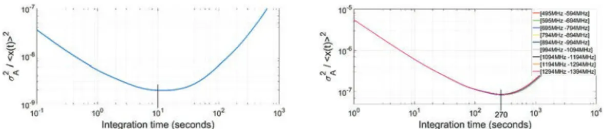
The Allan variance of the total signal, composed of the three noises, is the purple curve (figure3.3). For short integration times, the Allan variance mostly follows the white noise curve, because it is the dominant noise. At longer integration times, the white noise becomes negligible compared to the Flicker and drift noises, and the Allan variance increases due to the effect of the drift noise. The lowest noise level is obtained for an integration time corresponding to the minimum of the curve (where the Allan variance is the lowest), around 30 ms in our example. We call this optimal integration time or Allan time (TA). However, when the minimum is not clearly visible on the curve, a good estimation of the Allan time is when the Allan variance deviates from the radiometric line (White noise Allan variance) by a factorp2. Curves without distinct minimum can occur when the Flicker noise is important and the flat zone around the minimum of the Allan variance curve is quite large. The Allan variance is very useful to analyze the stability of an instrument because it enables us to clearly identify the 3 noises, and to exactly determine the optimum integration time.
3.2.2
Allan variance theory
The Allan variance theory is well described by Allan [31], Barnes [32], Schieder and Kramer [33] and Kooi [34]. The Allan variance of an instrument is defined by the Allan variance of data samples taken by this instrument when measuring a constant input signal (a load at constant temperature for example).
We consider a continuous data set composed of N contiguous data samples xi(i∈ [1 , N])), where the pauses between the measurements are negligible. The integration time of each data sample is τ. We look at subsets of K samples, each with an integration time of T = Kτ, where K is the number of xi samples considered. The N samples are split into M adjacent groups of K samples each (M = ⌊N/K⌋, where ⌊ ⌋ represents the f loor function). Each group is averaged and the calculated mean (Xn(K)) corresponds to the data measured by the instrument during an integration time T = Kτ.
Xn(K) = 1 K K X i=1 x(nK+i). (3.3)
σ2A(T ) = 〈(Xn+1(K)− Xn(K)) 2 〉 2 , (3.4) σA2(T ) = 1 2(M− 1) M−1 X n=1 (Xn+1(K)− Xn(K))2. (3.5)
To plot the Allan variance as a function of the integration time, we need to calculate σA2for different values of K (the number of samples averaged in one group). We iterate K from 1 to N/2 to calculate the Allan variance for integration times from τ to N τ/2. The successive Allan variance values calculated for different integration times (T = Kτ) constitute the Allan variance plot, as shown in figure3.4
FIGURE3.4: Schematic showing how the Allan variance is calculated by considering differ-ent groups of data samples. The Allan variance plot uses a log-log scale
3.2.2.1 Bandwidth influence on the Allan variance
The Allan variance also depends on the frequency bandwidth B of the measurement. As the bandwidth is increased (by averaging the signal of several channels of a spectrometer for example), the white noise is reduced. As a result, the Allan time (TA) becomes smaller because the intersection between the white noise and drift noise curves occurs at a shorter integration time. This relation is expressed by the following formula:
TA′ TA = B B′ β+11 , (3.6)
where β is the slope of the drift noise on the Allan variance plot, B and B′are two different bandwidths used to measure the same device, TAand TA′ are the two corresponding Allan