HAL Id: cea-01321792
https://hal-cea.archives-ouvertes.fr/cea-01321792
Submitted on 26 May 2016
HAL is a multi-disciplinary open access
archive for the deposit and dissemination of
sci-entific research documents, whether they are
pub-lished or not. The documents may come from
teaching and research institutions in France or
abroad, or from public or private research centers.
L’archive ouverte pluridisciplinaire HAL, est
destinée au dépôt et à la diffusion de documents
scientifiques de niveau recherche, publiés ou non,
émanant des établissements d’enseignement et de
recherche français ou étrangers, des laboratoires
publics ou privés.
real-space renormalization
Cécile Monthus
To cite this version:
Cécile Monthus. Dyson hierarchical long-ranged quantum spin-glass via real-space renormalization.
Journal of Statistical Mechanics, 2015, 2015 (10), pp.10024. �10.1088/1742-5468/2015/10/P10024�.
�cea-01321792�
arXiv:1506.06012v2 [cond-mat.dis-nn] 19 Sep 2015
via real-space renormalization
C´ecile MonthusInstitut de Physique Th´eorique, Universit´e Paris Saclay, CNRS, CEA, 91191 Gif-sur-Yvette, France We consider the Dyson hierarchical version of the quantum Spin-Glass with random Gaussian couplings characterized by the power-law decaying variance J2(r) ∝ r−2σ and a uniform transverse
field h. The ground state is studied via real-space renormalization to characterize the spinglass-paramagnetic zero temperature quantum phase transition as a function of the control parameter h. In the spinglass phase h < hc, the typical renormalized coupling grows with the length scale L as
the power-law JLtyp(h) ∝ Υ(h)L
θ with the classical droplet exponent θ = 1 − σ, where the stiffness
modulus vanishes at criticality Υ(h) ∝ (hc−h)µ, whereas the typical renormalized transverse field decays exponentially htypL (h) ∝ e−
L
ξ in terms of the diverging correlation length ξ ∝ (hc−h)−ν. At
the critical point h = hc, the typical renormalized coupling JLtyp(hc) and the typical renormalized
transverse field htypL (hc) display the same power-law behavior L−z with a finite dynamical exponent
z. The RG rules are applied numerically to chains containing L = 212 = 4096 spins in order to measure these critical exponents for various values of σ in the region 1/2 < σ < 1.
I. INTRODUCTION
In the field of classical spin-glasses, the Long-Ranged case of Gaussian couplings where the variance decays as a power-law of the distance r
J2(r) = 1
r2σ (1)
has been much studied recently [1–22] for various reasons : from the experimental point of view, the RKKY interaction in real spin-glasses actually decays as a power-law of the distance; from the numerical point of view, the Long-Ranged interaction can be studied in one dimension as a function of σ on much larger sizes than the case of Short-Ranged interaction as a function of the dimension d ; from the theoretical point of view, the Long-Ranged case is also easier to analyze via scaling arguments. In particular, within the droplet scaling theory [23, 24], the droplet exponent θ
governing the scaling of the renormalized random coupling JL with the length L
JL∝ Lθ (2)
is expected to be given by the exact simple formula [2, 24]
θLR(d, σ) = d − σ (3)
in the region where it is bigger than its short-ranged value θLR(d, σ) > θSR(d), whereas the short-ranged droplet
exponent θSR(d) is known only numerically as a function of d apart from the simple case θSR(d = 1) = −1. Since the
spin-glass phase is stable at low-temperature when the droplet exponent is positive θ > 0, and since the ground state energy is extensive for 2σ > d (Eq. 1), one obtains that the interesting region where the spin-glass phase exists up to
a finite temperature Tc
d
2 < σ < d (4)
exists already in dimension d = 1.
Besides the thermal transition of the classical spin-glass, it is also interesting to consider the effect of quantum fluctuations introduced by a uniform transverse-field h at zero temperature [25]
H = −X i hσiz− X (i,j) Ji,jσxiσxj (5)
where the Ji,j are the random couplings with the variance given by Eq. 1. For h = 0, one recovers the classical case
with the droplet exponent of Eq. 3, so that the region of interest is the same as in Eq. 4. For large h, the ground-state will be paramagnetic, so that one expects a quantum phase transition at zero temperature at some critical transverse
Fixed Point obtained via Strong Disorder Renormalization, either exactly in dimension d = 1 [26] or numerically in dimensions d = 2, 3, 4 [27–37] (Note that this Infinite Disorder Fixed Point can also be reproduced via real-space Block Renormalization [38, 39]). As a consequence, the relation with the power-law mean-field theory based on the properties of the infinite ranged model [40, 41] and supposed to apply in d > 8 [42] has remained unclear. However for the case of Long-Ranged couplings, the activated scaling of the renormalized couplings found at Infinite Disorder Fixed Point is not possible anymore, since the decay cannot be less than the initial power-law decay (Eq 1). As a consequence, the dynamical exponent z is finite, and one may expect more conventional power-law critical properties. The case of the Long-Ranged random ferromagnetic quantum Ising chain has been studied recently both via Strong Disorder Renormalization [43–45] and via Block Renormalization [46]. The aim of the present paper is to study the properties of the Long-Ranged quantum spin-glass chain via the block real-space renormalization used previously for the ferromagnetic case [46].
The paper is organized as follows. In section II, we describe the real-space renormalization rules for the Dyson hierarchical version of the quantum Long-Ranged Spin-Glass model, and solve them deep in the spinglass phase and deep in the paramagnetic phase. In section III, the RG rules are applied numerically in the critical region to measure the critical behaviors. Our conclusions are summarized in section IV.
II. REAL-SPACE RENORMALIZATION APPROACH A. Dyson hierarchical Quantum Long-Ranged Spin-Glass model
Since the studies concerning the Dyson hierarchical classical ferromagnetic Ising model [47–56], many long-ranged disordered models have been analyzed via their Dyson hierarchical analogs including for instance random fields Ising models [57–59] and Anderson localization models [60–67]. Here we start from the Dyson hierarchical classical spin-glass model [68–74] and we simply add transverse fields to introduce quantum fluctuations. More precisely, the Dyson
hierarchical Quantum Spin-Glass model for N = 2n spins is defined as a sum over the generations k = 0, 1, .., n − 1
H(1,2n) =
n−1
X
k=0
H(1,2(k)n) (6)
The Hamiltonian of generation k = 0 contains the transverse fields hi and the lowest order couplings J
(0) 2i−1,2i H(1,2(k=0)n) = − 2n X i=1 hiσiz− 2n−1 X i=1 J2i−1,2i(0) σx2i−1σ2ix (7)
The Hamiltonian of generation k = 1 reads
H(1,2(k=1)n) = − 2n−2 X i=1 h J4i−3,4i−1(1) σx 4i−3σ4i−1x + J (1) 4i−3,4iσ4i−3x σ4ix + J (1)
4i−2,4i−1σ4i−2x σ4i−1x + J
(1)
4i−2,4iσ4i−2x σ4ix
i (8) and so on up to the last generation k = n − 1 that couples all pairs of spins between the two halves of the system
H(1,2(n−1)n) = − 2n−1 X i=1 2n X j=2n−1+1 Ji,j(n−1)σixσjx (9)
At generation k, associated to the length scale Lk= 2k, the couplings J
(k)
i,j read
Ji,j(k)= ∆kǫij (10)
where ǫij are independent random variables of zero mean drawn with the Gaussian distribution
G(ǫ) = √1
4πe
−ǫ2
4 (11)
The characteristic scale ∆k is chosen to decay exponentially with the number k of generations, in order to mimic the
power-law decay of Eq. 1 with respect to the length scale Lk = 2k
∆k = 2−kσ =
1
Lσ
k
Then one expects that many scaling properties will be the same. In particular, in the absence of the transverse fields, the classical ground state is characterized by the same droplet exponent of Eq. 3 for d = 1 (see more details in [19, 20])
θ(σ) = 1 − σ (13)
Here we will consider the case where all the transverse field hiin Eq. 7 are all equal initially
hi= h (14)
so that this value h represents the control parameter of the spinglass-paramagnetic transition. Upon renormalization however, the renormalized transverse field will become random variables as we now describe.
B. Renormalization procedure
We use the same renormalization procedure as in our previous work concerning the ferromagnetic case [46]. The only technical difference in the derivation of the RG rules is that we have to take into account the random amplitude and the random sign of the couplings. But of course the physical properties obtained from the RG flows will be completely different as expected for a spin-glass model.
The elementary renormalization step concerns the box two-spin Hamiltonian of generation k = 0 of Eq. 7
H(2i−1,2i) = −h2i−1σ2i−1z − h2iσz2i− J
(0)
2i−1,2iσx2i−1σ2ix (15)
Within the symmetric sector
H(2i−1,2i)| + + > = −(h2i−1+ h2i)| + + > −J2i−1,2i(0) | − − >
H(2i−1,2i)| − − > = −J2i−1,2i(0) | + + > +(h2i−1+ h2i)| − − > (16)
we project out the highest eigenvalue λS+2i = +q(J2i−1,2i(0) )2+ (h
2i−1+ h2i)2 to keep only the lowest eigenvalue
λS−2i = −
q
(J2i−1,2i(0) )2+ (h2i−1+ h2i)2 (17)
corresponding to the eigenvector
|λS−2i > = cos θ2iS| + + > + sin θS2i| − − > (18)
in terms of the angle θS satisfying
cos(θS 2i) = v u u t 1 + h2i−1+h2i q (J2i−1,2i(0) )2+(h 2i−1+h2i)2 2 sin(θS 2i) = sgn(J (0) 2i−1,2i) v u u t 1 − h2i−1+h2i q (J2i−1,2i(0) )2+(h 2i−1+h2i)2 2 (19)
Similarly within the antisymmetric sector
H(2i−1,2i)| + − > = −(h2i−1− h2i)| + − > −J2i−1,2i(0) | − + >
H(2i−1,2i)| − + > = −J
(0)
2i−1,2i| + − > +(h2i−1− h2i)| − + > (20)
we project out the highest eigenvalue λA+2i = +
q
(J2i−1,2i(0) )2+ (h2i−1− h2i)2to keep only the lowest eigenvalue
λA−
2i = −
q
(J2i−1,2i(0) )2+ (h
2i−1− h2i)2 (21)
with the corresponding eigenvector
|λA−
in terms of the angle θA satisfying cos(θA 2i) = v u u t 1 + h2i−1−h2i q (J2i−1,2i(0) )2+(h 2i−1−h2i)2 2 sin(θA2i) = sgn(J (0) 2i−1,2i) v u u t 1 − h2i−1−h2i q (J2i−1,2i(0) )2+(h 2i−1−h2i)2 2 (23)
In summary, for each two-spin Hamiltonian H2i−1,2i of Eq. 15, we keep only the two lowest states and label them as
the two states of some renormalized spin σR(2i)
|σz R(2i)= + > ≡ |λ S− 2i > |σz R(2i)= − > ≡ |λA−2i > (24)
It is convenient to introduce the corresponding spin operators σz
R(2i) ≡ |σzR(2i)= + >< |σzR(2i)= +| − |σzR(2i)= − >< σzR(2i)= −|
σx
R(2i) ≡ |σzR(2i)= + >< |σzR(2i)= −| + |σzR(2i)= − >< σzR(2i)= +| (25)
and the projector
P−
2i ≡ |σzR(2i)= + >< |σzR(2i)= +| + |σzR(2i)= − >< σzR(2i)= −| (26)
C. Renormalization rule for the transverse fieldshR(2i)
The projection of the Hamiltonian of Eq. 15 reads
P−
2iH(2i−1,2i)P
−
2i = λS−2i |λS−2i >< λS−2i | + λA−2i |λA−2i >< λA−2i |
= λ S− 2i + λA−2i 2 ! P− 2i + λS−2i − λA−2i 2 ! σz R(2i) (27)
so that the renormalized transverse field defined as the coefficient of (−σz
R(2i)) is given by hR(2i) = λA−2i − λS−2i 2 ! = q 2h2i−1h2i (J2i−1,2i(0) )2+ (h 2i−1+ h2i)2+ q (J2i−1,2i(0) )2+ (h 2i−1− h2i)2 (28)
D. Renormalization rules for the couplingsJR(2i),R(2j)
The projection of the σx operators
P− 2iσ2i−1x P − 2i = c2i−1σR(2i)x P− 2iσ2ixP − 2i = c2iσxR(2i) (29)
involves the two coefficients
c2i−1 = sgn(J2i−1,2i(0) ) v u u u t 1 + (J (0) 2i−1,2i)2−h 2 2i−1+h 2 2i q (J2i−1,2i(0) )2+(h 2i−1+h2i)2 q (J2i−1,2i(0) )2+(h 2i−1−h2i)2 2 c2i = v u u u t 1 + (J (0) 2i−1,2i)2+h22i−1−h22i q (J2i−1,2i(0) )2+(h 2i−1+h2i)2 q (J2i−1,2i(0) )2+(h 2i−1−h2i)2 2 (30)
The renormalized coupling between σR(2i) and σR(2j) is then given by the following linear combination of the four
initial couplings of generation k associated to the positions (2i − 1, 2i) and ((2j − 1, 2j)
JR(2i),R(2j) = J (k) 2i,2jc2ic2j+ J (k) 2i−1,2jc2i−1c2j+ J (k) 2i,2j−1c2ic2j−1+ J (k) 2i−1,2j−1c2i−1c2j−1 (31)
E. Iteration of the elementary renormalization step
In summary, the elementary renormalization step described above maps the initial model containing L = 2n spins
(σ1, ..., σ2n) with their transverse fields hiand their couplings Ji,j(k)into a renormalized model containingL
2 = 2
n−1spins
(σR(2), ..., σR(2n)) with their renormalized transverse fields hR(2i) given by Eq. 28 and their renormalized couplings
JR(2i),R(2j) given by Eq. 31. The iteration is now straightforward : the next renormalization step will produce a
renormalized model containing L
4 = 2
n−2 spins (σ
R2(4), ..., σR2(2n)) with their renormalized transverse fields hR2(4i)
and their renormalized couplings JR2(4i),R2(4j), etc. The renormalization procedure ends after n RG steps where the
whole sample containing L = 2n initial spins has been renormalized into a single renormalized spin σ
Rn(2n).
F. RG flows deep in the Spin-Glass phase
Deep in the Spin-Glass phase, the transverse fields hi are negligible with respect to the couplings Ji,j. As a
consequence, the coefficients of Eq. 30 reduce to
c2i−1 ≃ sgn(J2i−1,2i(0) )
c2i ≃ 1 (32)
and the RG rule for the renormalized coupling of Eq. 31 becomes
JR(2i),R(2j) = J2i,2j+ J2i−1,2jsgn(J2i−1,2i(0) ) + J2i,2j−1sgn(J2j−1,2j(0) ) + J2i−1,2j−1sgn(J2i−1,2i(0) )sgn(J
(0)
2j−1,2j) (33)
This rule coincides with the RG rule for the classical spin-glass at zero temperature studied in detail in [19, 20], and in particular, the variance evolves according to
(JR
R(2i),R(2j))2≃ 4J
2
2i,2j (34)
In terms of the length L = 2n obtained after n RG steps, the variance grows as
(JR
L)2≃ 4nL
−2σ= L2−2σ
≡ L2θ (35)
with the droplet exponent of Eq. 13
θ = 1 − σ (36)
in agreement with the exact simple formula of Eq. 3 predicted via scaling arguments [2, 24] and numerically measured via Monte-Carlo [3].
The RG rule of Eq. 28 for the transverse field simplifies into
hR(2i) ≃
h2i−1h2i
|J2i−1,2i(0) |
(37) and is thus analogous to the usual Strong Disorder RG rule concerning a strong-bond-decimation [26]. The iteration of this rule in log-variables
ln hR(2i) ≃ ln h2i−1+ ln h2i− ln |J2i−1,2i(0) | (38)
yields that the disorder average decays linearly in the length L = 2n obtained after n RG steps
ln hL ≃ −(cst)L (39)
whereas the variance grows as in the Central Limit theorem
(ln hL)2− (ln hL)2 ∝ L
1
G. RG flows deep in the Paramagnetic phase
Deep in the paramagnetic phase, the couplings Ji,j are negligible with respect to the transverse fields hi. As a
consequence, the renormalized transverse fields of Eq. 28 remain all equal to their common initial value h (Eq. 28)
hR(2i) ≃ h (41)
whereas the coefficients of Eq. 30 simplify into
c2i−1 ≃ sgn(J2i−1,2i(0) ) 1 √ 2 c2i ≃ 1 √ 2 (42)
so that the RG rule for the renormalized coupling of Eq. 31 becomes
JR(2i),R(2j) =
1 2 h
J2i,2j+ J2i−1,2jsgn(J2i−1,2i(0) ) + J2i,2j−1sgn(J2j−1,2j(0) ) + J2i−1,2j−1sgn(J2i−1,2i(0) )sgn(J
(0)
2j−1,2j)
i (43) In particular, the variance remains stable
(JR
R(2i),R(2j))2≃ J2i,2j2 (44)
i.e. the renormalized couplings keep the same decay as the original couplings
(JR
L)2≃ L
−2σ (45)
III. NUMERICAL STUDY OF THE CRITICAL PROPERTIES
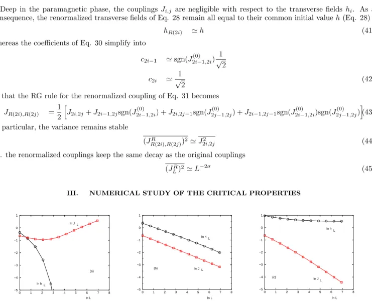
0 1 2 3 4 5 6 7 8 −5 −4 −3 −2 −1 0 1 ln L ln J L ln h L (a) 0 1 2 3 4 5 6 7 8 −5 −4 −3 −2 −1 0 1 ln L ln hL ln J L (b) 0 1 2 3 4 5 6 7 8 −5 −4 −3 −2 −1 0 1 (c) ln L ln h L ln JL
FIG. 1: RG flows in log-log scale of the typical renormalized transverse field htypL (circles) and of the renormalized coupling
Jtyp
L (squares) for σ = 0.625 :
(a) in the spin-glass phase (example here with h = 1.0), the coupling grows as JLtyp∝Υ(h)L1−σ whereas the transverse field decays exponentially htypL ∝e
−Lξ.
(b) at the critical point hc= 1.78, JLtypand h typ
L decay with the same power-law of exponent z (Eq. 47)
(c) in the paramagnetic phase (example here with h = 3.0), the coupling JLtypdecays, whereas htypL converges towards a finite value.
A. Numerical details
We have applied numerically the renormalization rules to ns = 13.103 disordered samples containing N = 212 =
4096 spins, corresponding to 12 generations. For each renormalization step corresponding to the lengths L = 2n
with n = 1, 2, .., 12 we have analyzed the statistical properties of the renormalized transverse fields hL and of the
renormalized couplings JL. In particular, we have measured the RG flows of the corresponding typical values
ln htypL ≡ ln hL
ln JLtyp ≡ ln |JL| (46)
as a function of the length L for various values of the initial transverse field h that represents the control parameter of the spinglass-paramagnetic transition.
B. Location of the critical point and measure of the dynamical exponentz
The critical point hc corresponds to the unstable fixed point where the transverse fields and the couplings remain
in competition at all scales (see Fig. 1). When this happens, both typical values of Eq. 46 decay as a power-law with the dynamical exponent z
ln htypL (hc) ∝ −z ln L
ln JLtyp(hc) ∝ −z ln L (47)
For the four values σ = 0.55, σ = 5/8 = 0.625, σ = 0.75 and σ = 0.9 that we have studied, our numerical data for the
critical point hc and for the dynamical exponent are given in the Table I.
σ Critical Point hc Dynamical exponent z Stiffness modulus exponent µ Correlation length exponent ν ω Gap exponent g
0.55 2.04 0.31 1.9 2.5 0.6 0.77
0.625 1.78 0.36 1.72 2.34 0.62 0.84
0.75 1.46 0.46 1.52 2.14 0.62 0.98
0.9 1.19 0.58 1.3 1.9 0.6 1.1
TABLE I: Numerical estimates of the critical point hc, of the dynamical exponent z, of the stiffness modulus exponent µ, of
the correlation length exponent ν, of ω and of the gap exponent g for four values of the parameter σ.
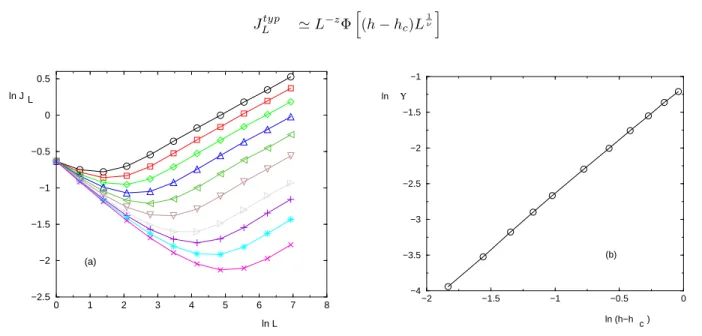
C. Finite-size scaling of the renormalized typical coupling
We now consider the finite-size scaling form of the typical renormalized coupling
JLtyp ≃ L−zΦh(h − h c)L 1 ν i (48) 0 1 2 3 4 5 6 7 8 −2.5 −2 −1.5 −1 −0.5 0 0.5 ln L ln J L (a) −2 −1.5 −1 −0.5 0 −4 −3.5 −3 −2.5 −2 −1.5 −1 ln (h−h c) Υ (b) ln
FIG. 2: Critical behavior of the stiffness modulus (Eq. 50) for σ = 0.75 :
(a) RG flow in log-log scale of the renormalized coupling for various values of the initial transverse field h in the spin-glass phase h < hc [namely h = 0.5 (circle); h = 0.6 (square);) h = 0.7 (diamond); h = 0.8 (triangle up); h = 0.9 (triangle left);
h = 1.0 (triangle down); h = 1.1 (triangle right); h = 1.15 (plus); h = 1.2 (star); h = 1.25 (cross)] : the asymptotic growth as ln Jtyp
L = (1 − σ) ln L + ln Υ(h) (Eq. 49) allows to extract the stiffness modulus Υ(h) as a function of the control parameter h
(b) ln Υ(h) as a function of ln(hc−h) yields the slope µ ≃ 1.52
In the spin-glass phase h < hc, the typical value of the renormalized coupling grows as a power-law of exponent
θ = 1 − σ (Eq. 36)
JLtyp|h<hc ∝
L→+∞Υ(h)L
where the stiffness modulus Υ(h) vanishes as a power-law
Υ(h) ∝
h→hc
(hc− h)µ (50)
The matching between Eq. 47 and Eq. 49 via the finite-size scaling form of Eq. 48 yields the relation between critical exponents
µ
ν = 1 − σ + z (51)
Our numerical data in the spin-glass phase (see Fig. 2) follow the power-laws of 49 and 50 with the exponent µ given in Table I. The corresponding numerical values for the correlation length exponent ν = µ/(1 − σ + z) (Eq. 51) are also given in Table I. We find that these values yield very satisfactory finite-size scaling with Eq. 48 of our numerical data (see for instance Fig. 3 for the case σ = 0.75).
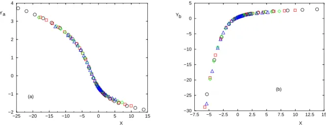
−25 −20 −15 −10 −5 0 5 10 15 −2 −1 0 1 2 3 4 X Ya (a) −7.5 −5 −2.5 0 2.5 5 7.5 10 12.5 15 −30 −25 −20 −15 −10 −5 0 5 X Yb (b)
FIG. 3: Finite-size scaling for σ = 0.75 with the dynamical exponent z = 0.46 and the correlation length exponent ν = 2.14 shown here for the four bigger sizes L = 4096 (circles), L = 2048 (squares), L = 1024 (diamond) and L = 512 (triangles) (a) Test of Eq 48 : Ya= ln JLtyp+ z ln L as a function of X = (h − hc)L
1 ν
(b) Test of Eq 55 : Yb= ln htypL + z ln L as a function of X = (h − hc)L
1 ν
In the paramagnetic phase h > hc, the typical renormalized coupling keeps the initial power-law behavior (Eq. 45)
JLtyp|h>hc ∝
L→+∞
A(h)
Lσ (52)
where the amplitude diverges at criticality
A(h) ∝
h→hc(h − h
c)−ω (53)
The matching between 47 and Eq. 52 finite-size scaling form of Eq. 48 via the finite-size scaling form of Eq. 48 yields the relation
ω
ν + z = σ (54)
The previous estimates lead to the values ω = ν(σ − z) (see Table I).
D. Finite-size scaling of the renormalized transverse field
The typical renormalized transverse field is expected to follow the following finite-size scaling form analog to Eq. 48 htypL ≃ L−zΨh(h − h c)L 1 ν i (55)
The corresponding finite-size scaling of our numerical data is shown on Fig. 3 (b) for the case σ = 0.75.
In the Spin-Glass phase h < hc, the leading exponential decay of the typical transverse field (Eq. 39) allows to
define some correlation length ξ(h)
ln htypL |h<hc = ln hL ∝
L→+∞−
L
ξ(h) (56)
The divergence near criticality involve the correlation exponent ν of Eq. 55
ξ(h) ∝
h→hc
(hc− h)−ν (57)
In the paramagnetic phase h > hc, the typical renormalized transverse field converges towards a finite asymptotic
value
htypL |h>hc ∝
L→+∞h
typ
∞ (h) (58)
that vanishes as a power-law
htyp
∞ ∝
h→hc(h − h
c)g (59)
The matching between Eq. 55 and Eq. 58 yields the standard relation for the gap critical exponent
g = zν (60)
The previous estimates lead to the values given in Table I.
E. Link with the standard critical exponents (α, β, γ, η)
Up to now, we have described the critical exponents involved in the RG flows of the transverse fields and of the couplings. It seems now useful to describe the link with the standard critical exponents (α, β, η, γ) of the general theory of critical phenomena [75, 76] :
(i) the exponent α governing the singular part of the ground state energy
eGS∝ |h − hc|2−α (61)
can be obtained via the quantum hyperscaling relation involving the spatial dimensionality d = 1 and the dynamical exponent z [75]
2 − α = ν(d + z) = ν(1 + z) (62)
Our numerical data leads to the negative values given in Table II for the exponent α. (ii) the exponent β governing the vanishing of the Edwards-Anderson order parameter
qEA≡ < σxi >2∝ |h − hc|β (63)
yields the following finite-size scaling decay at criticality
qEA(L) ∝ L−
β
ν (64)
The relation with the scaling of the renormalized coupling
J2(L) ∝ L−2z
≃ Jini2 (L)(LqEA)2∝ L−2σ+2−2
β
ν (65)
yields the relation
β
ν = 1 − σ + z (66)
The comparison with Eq. 51 shows that β actually coincides with the exponent µ of the stiffness modulus
(iii) the correlation exponent η governing the power-law decay of the equal-time spatial correlation function at criticality [75, 76]
C(r) ≡ < σx
iσxi+r>2∝ r
−(d+z−2+η) (68)
is related by finite-size scaling to the sqare of the order parameter q2
EA(L) ∝ L
−2βν leading to
d + z − 2 + η = 2βν = 2(1 − σ + z) (69)
so that here with d = 1, one obtains
η = 3 − 2σ + z (70)
(iv) the experimentally measurable non-linear susceptibility χnl scales as
χnl∝ L γnl ν (71) with [76, 77] γnl ν = 2 − η + 2z = (2σ − 1) + z (72)
whereas the overlap susceptibility involves the exponent [76]
γoverlap
ν = 2 − η + z = 2σ − 1 (73)
and the spin-glass susceptibility involves [76, 77]
γSG
ν = 2 − η = 2σ − 1 − z (74)
We refer to References [76, 77] for more details on these various susceptibilities involving different numbers of inte-gration in the time direction.
(v) the time-autocorrelation decays at criticality as the power-law < σx
i(0)σxi(t) > ∝ t
−ρ (75)
with the finite-size-scaling value
ρ = β
νz = 1 +
1 − σ
z (76)
The numerical results of the RG flows given in Table I thus translate into the values given in Table II for the standard exponents of phase transitions just described.
σ α β η γnl γoverlap γSG ρ
0.55 -1.27 1.9 2.21 0.41 0.1 -0.21 2.45 0.625 -1.18 1.72 2.11 0.61 0.25 -0.11 2.04 0.75 -1.12 1.52 1.96 0.96 0.5 0.04 1.54 0.9 -1.0 1.3 1.78 1.38 0.8 0.22 1.17
TABLE II: Numerical estimates of the standard exponents of the phase transition as obtained via scaling relations from the numerical results of Table I.
IV. CONCLUSION
In this paper, we have studied via real-space renormalization the ground state of the Dyson hierarchical version
of the quantum Long-Ranged Spin-Glass with the power-law decaying variance J2(r) ∝ r−2σ. In particular, we
transverse field h. In the spinglass phase h < hc, the typical renormalized coupling grows with the length scale L
as the power-law JLtyp(h) ∝ Υ(h)Lθ with the classical droplet exponent θ = 1 − σ whereas the typical renormalized
transverse field decays exponentially htypL (h) ∝ e−L
ξ. At the critical point h = h
c, the typical renormalized coupling
JLtyp(hc) and the typical renormalized transverse field htypL (hc) display the same power-law behavior L−zwith a finite
dynamical exponent z. The RG rules have been applied numerically to chains containing L = 212 = 4096 spins in
order to measure the critical exponents for various values of σ in the interesting region 1/2 < σ < 1.
We hope that the present work will motivate other studies on the quantum SpinGlass-Paramagnetic transition at zero temperature in the presence of Long-Ranged couplings. In particular it would be very interesting the compare with values of critical exponents obtained via Monte-Carlo simulations or other numerical methods.
[1] G. Kotliar, P.W. Anderson and D.L. Stein, Phys. Rev. B 27, 602 (1983). [2] A.J. Bray, M.A. Moore and A.P. Young, Phys. Rev. Lett. 56, 2641 (1986). [3] H.G. Katzgraber and A.P. Young, Phys. Rev. B 67, 134410 (2003). [4] H.G. Katzgraber and A.P. Young, Phys. Rev. B 68, 224408 (2003).
[5] H.G. Katzgraber, M. Korner, F. Liers and A.K. Hartmann, Prog. Theor. Phys. Sup. 157, 59 (2005). [6] H.G. Katzgraber, M. Korner, F. Liers, M. Junger and A.K. Hartmann, Phys. Rev. B 72, 094421 (2005). [7] H.G. Katzgraber, J. Phys. Conf. Series 95, 012004 (2008).
[8] H. G. Katzgraber and A. P. Young, Phys. Rev. B 72, 184416 (2005). [9] A.P. Young, J. Phys. A 41, 324016 (2008).
[10] H. G. Katzgraber, D. Larson and A. P. Young, Phys. Rev. Lett. 102, 177205 (2009). [11] M.A. Moore, Phys. Rev. B 82, 014417 (2010).
[12] H.G. Katzgraber, A.K. Hartmann and and A.P. Young, Physics Procedia 6, 35 (2010). [13] H.G. Katzgraber and A.K. Hartmann, Phys. Rev. Lett. 102, 037207 (2009);
H.G. Katzgraber, T. Jorg, F. Krzakala and A.K. Hartmann, Phys. Rev. B 86, 184405 (2012). [14] T. Mori, Phys. Rev. E 84, 031128 (2011).
[15] M. Wittmann and A. P. Young, Phys. Rev. E 85, 041104 (2012) [16] C. Monthus and T. Garel, Phys. Rev. B 88, 134204 (2013). [17] C. Monthus and T. Garel, Phys. Rev. B 89, 014408 (2014). [18] C. Monthus and T. Garel, J. Stat. Mech. P03020 (2014). [19] C. Monthus, J. Stat. Mech. P06015 (2014).
[20] C. Monthus, J. Stat. Mech. P08009 (2014). [21] M. Wittmann and A. P. Young, arXiv:1504.07709. [22] A. Billoire, arXiv:1505.00676.
[23] A.J. Bray and M. A. Moore, J. Phys. C 17 (1984) L463;
A.J. Bray and M. A. Moore, “Scaling theory of the ordered phase of spin glasses” in Heidelberg Colloquium on glassy dynamics, edited by JL van Hemmen and I. Morgenstern, Lecture notes in Physics vol 275 (1987) Springer Verlag, Heidelberg.
[24] D.S. Fisher and D.A. Huse, Phys. Rev. B38, 386 (1988); D.S. Fisher and D.A. Huse, Phys. Rev B38, 373 (1988). [25] A. Dutta, Phys. Rev. B 65, 224427 (2002).
[26] D. S. Fisher, Phys. Rev. Lett. 69, 534 (1992); Phys. Rev. B 51, 6411 (1995). [27] D. S. Fisher, Physica A 263, 222 (1999).
[28] O. Motrunich, S.-C. Mau, D. A. Huse, and D. S. Fisher, Phys. Rev. B 61, 1160 (2000). [29] Y.-C. Lin, N. Kawashima, F. Igloi, and H. Rieger, Prog. Theor. Phys. 138, 479 (2000). [30] D. Karevski, YC Lin, H. Rieger, N. Kawashima and F. Igloi, Eur. Phys. J. B 20, 267 (2001). [31] Y.-C. Lin, F. Igloi, and H. Rieger, Phys. Rev. Lett. 99, 147202 (2007).
[32] R. Yu, H. Saleur, and S. Haas, Phys. Rev. B 77, 140402 (2008). [33] I. A. Kovacs and F. Igloi, Phys. Rev. B 80, 214416 (2009). [34] I. A. Kovacs and F. Igloi, Phys. Rev. B 82, 054437 (2010). [35] I. A. Kovacs and F. Igloi, Phys. Rev. B 83, 174207 (2011). [36] I. A. Kovacs and F. Igloi, arXiv:1108.3942.
[37] I. A. Kovacs and F. Igloi, J. Phys. Condens. Matter 23, 404204 (2011).
[38] R. Miyazaki, H. Nishimori and G. Ortiz, Phys. Rev. E 83, 051103 (2011). R. Miyazaki and H. Nishimori, Phys. Rev. E 87, 032154 (2013).
[39] C. Monthus, J. Stat. Mech. P01023 (2015).
[40] A.J. Bray and M.A. Moore, J. Phys. C Solid Atate Phys. 13, L655 (1980). [41] J. Miller and D.A. Huse, Phys. Rev. Lett. 70, 3147 (1993).
[42] N. Read, S. Sachdev and J. Ye, Phys. Rev. B 52, 384 (1995). [43] R. Juhasz, I. A. Kovacs and F. Igloi, EPL, 107 (2014) 47008.
[44] R. Juhasz, J. Stat. Mech. (2014) P09027.
[45] R. Juhasz, I. A. Kovacs and F. Igloi, Phys. Rev. E 91, 032815 (2015). [46] C. Monthus, J. Stat. Mech. P05026 (2015).
[47] F. J. Dyson, Comm. Math. Phys. 12, 91 (1969) and 21, 269 (1971).
[48] P.M. Bleher and Y.G. Sinai, Comm. Math. Phys. 33, 23 (1973) and Comm. Math. Phys. 45, 247 (1975); Ya. G. Sinai, Theor. and Math. Physics, Volume 57,1014 (1983) ;
P.M. Bleher and P. Major, Ann. Prob. 15, 431 (1987) ; P.M. Bleher, arXiv:1010.5855.
[49] G. Gallavotti and H. Knops, Nuovo Cimento 5, 341 (1975).
[50] P. Collet and J.P. Eckmann, “A Renormalization Group Analysis of the Hierarchical Model in Statistical Mechanics”, Lecture Notes in Physics, Springer Verlag Berlin (1978).
[51] G. Jona-Lasinio, Phys. Rep. 352, 439 (2001). [52] G.A. Baker, Phys. Rev. B 5, 2622 (1972);
G.A. Baker and G.R. Golner, Phys. Rev. Lett. 31, 22 (1973); G.A. Baker and G.R. Golner, Phys. Rev. B 16, 2081 (1977);
G.A. Baker, M.E. Fisher and P. Moussa, Phys. Rev. Lett. 42, 615 (1979). [53] J.B. McGuire, Comm. Math. Phys. 32, 215 (1973).
[54] A J Guttmann, D Kim and C J Thompson, J. Phys. A: Math. Gen. 10 L125 (1977); D Kim and C J Thompson J. Phys. A: Math. Gen. 11, 375 (1978) ;
D Kim and C J Thompson J. Phys. A: Math. Gen. 11, 385 (1978); D Kim, J. Phys. A: Math. Gen. 13 3049 (1980).
[55] D Kim and C J Thompson J. Phys. A: Math. Gen. 10, 1579 (1977). [56] C. Monthus and T. Garel, J. Stat. Mech. P02023 (2013).
[57] G J Rodgers and A J Bray, J. Phys. A: Math. Gen. 21 2177 (1988). [58] C. Monthus and T. Garel, J. Stat. Mech. P07010 (2011).
[59] G. Parisi and J. Rocchi, Phys. Rev. Lett. 90, 02403 (2014);
A. Decelle, G. Parisi and J. Rocchi, Phys. Rev. E 89, 032132 (2014). [60] A. Bovier, J. Stat. Phys. 59, 745 (1990).
[61] S. Molchanov, ’Hierarchical random matrices and operators, Application to the Anderson model’ in ’Multidimensional statistical analysis and theory of random matrices’ edited by A.K. Gupta and V.L. Girko, VSP Utrecht (1996).
[62] E. Kritchevski, Proc. Am. Math. Soc. 135, 1431 (2007) and Ann. Henri Poincare 9, 685 (2008);
E. Kritchevski ’Hierarchical Anderson Model’ in ’Probability and mathematical physics : a volume in honor of S. Molchanov’ edited by D. A. Dawson et al. , Am. Phys. Soc. (2007).
[63] S. Kuttruf and P. M¨uller, Ann. Henri Poincare 13, 525 (2012)
[64] Y.V. Fyodorov, A. Ossipov and A. Rodriguez, J. Stat. Mech. L12001 (2009). [65] E. Bogomolny and O. Giraud, Phys. Rev. Lett. 106, 044101 (2011).
[66] I. Rushkin, A. Ossipov and Y.V. Fyodorov, J. Stt. Mech. L03001 (2011). [67] C. Monthus and T. Garel, J. Stat. Mech. P05005 (2011).
[68] S. Franz, T. Jorg and G. Parisi, J. Stat. Mech. P02002 (2009).
[69] M. Castellana, A. Decelle, S. Franz, M. M´ezard and G. Parisi, Phys. Rev. Lett. 104, 127206 (2010). [70] M. Castellana and G. Parisi, Phys. Rev. E 82, 040105(R) (2010) ;
M. Castellana and G. Parisi, Phys. Rev. E 83, 041134 (2011) . [71] M. Castellana, Europhysics Letters 95 (4) 47014 (2011).
[72] M.C. Angelini, G. Parisi and F. Ricci-Tersenghi, Phys. Rev. B 87, 134201 (2013). [73] M. Castellana, A. Barra and F. Guerra, J. Stat. Phys. 155, 211 (2014).
[74] M. Castellana and C. Barbieri, Phys. Rev. B 91, 024202 (2015). [75] M.J. Thill and D.A. Huse, Physica A 214, 321 (1995).
[76] H. Rieger and A.P. Young, Phys. Rev. Lett. 72, 4141 (1994);
H. Rieger and A.P. Young, “Coherent approach to fluctuations”, ed . M. Susuki and N. Nawashima, World Scientific, Singapore (1996).