HAL Id: hal-03214963
https://hal.inria.fr/hal-03214963
Submitted on 3 May 2021
HAL is a multi-disciplinary open access archive for the deposit and dissemination of sci-entific research documents, whether they are pub-lished or not. The documents may come from teaching and research institutions in France or abroad, or from public or private research centers.
L’archive ouverte pluridisciplinaire HAL, est destinée au dépôt et à la diffusion de documents scientifiques de niveau recherche, publiés ou non, émanant des établissements d’enseignement et de recherche français ou étrangers, des laboratoires publics ou privés.
Couplings Using Continuation Method
Yan Zhang, Ke-Li Wu, Fabien Seyfert
To cite this version:
Yan Zhang, Ke-Li Wu, Fabien Seyfert. A Direct Preconditioner for Coupling Matrix Reconfiguration of Bandpass Filters With Irregular Couplings Using Continuation Method. IEEE Transactions on Microwave Theory and Techniques, Institute of Electrical and Electronics Engineers, 2021, 69 (2), pp.1394-1403. �10.1109/TMTT.2020.3045991�. �hal-03214963�
Abstract—In this paper, a direct preconditioner is proposed for coupling matrix reconfiguration of bandpass filters with irregular couplings using the coefficient-parameter continuation method. With the preconditioner, the continuation method can be effectively used for filter synthesis and model extraction of bandpass filters with irregular couplings. In dealing with practical filters that contain a coupling topology with regular cross couplings introduced intentionally or unintentionally, the proposed preconditioner, being used as the start system in the continuation method, can swiftly lead to the solution that matches the physical realization. The preconditioner is physics-based and can be easily obtained by reconfiguring the regular coupling topology with the conventional method. The continuation process with a coefficient-parameter homotopy for coupling matrix reconfiguration is formulated for the first time, which transforms a coupling matrix in canonical form to that in the desired one with irregular couplings. The convergence of the solution and a bootstrapping approach for dealing with multiple irregular couplings are also discussed. The method provides an enabling tool for robot automatic tuning (RAT) of advanced microwave bandpass filters. Three practical examples are presented, including one synthesis example and two model extraction examples for RAT, demonstrating the effectiveness of the reconfiguration method for practical applications.
Index Terms—Coupling matrix, filter reconfiguration, homotopy continuation, irregular topologies, microwave filter tuning, preconditioner.
I. INTRODUCTION
UNING of high-performance microwave filters is inevitable due to stringent electrical specifications. The labor-intensive manual tuning process, being time-consuming and costly, motivates the recent development of computer-aided tuning (CAT) and robot automatic tuning (RAT), for which coupling matrix [1] is used as the bridge between the physical model and the circuit model of the filter realization in the filter domain. In a robust RAT system, extraction of a legitimate circuit model contains three major
Manuscript received May 7, 2020. The work described in this paper was substantially supported by the Hong Kong Ph.D Fellowship. (Corresponding author: Ke-Li Wu.)
Yan Zhang and Ke-Li Wu are with the Department of Electronic Engineering, The Chinese University of Hong Kong, Shatin, Hong Kong (e-mail: [email protected]; [email protected]). Fabien Seyfert is with INRIA, Sophia-Antipolis, France, (e-mail: [email protected]).
steps: 1) to obtain the filtering function characterized by three polynomials from the measured response; 2) to transform the filtering function into the circuit model (coupling matrix) in a canonical form; and 3) to reconfigure the coupling matrix in the canonical form to that in the coupling topology that best fits the physical realization. The third step is usually conducted through a sequence of orthogonal transformations. The subsequent tuning strategy of the filter will depend on the difference between the extracted and the target coupling matrices. Among the three steps, the system identification problem in the first step can be addressed using well-developed methods, such as vector fitting [2] and the recently proposed model-based vector fitting (MVF) methods [3]. As long as a set of sensible filtering functions are obtained, a unique coupling matrix in a canonical form can be derived straightforwardly in the second step. However, coupling matrix reconfiguration in the third step using well-established orthogonal transformations [4] is limited to the conventional regular coupling topologies, such as those constructed by cascaded trisections (CTs) and cascaded quartets (CQs) [5].
The demands for dealing with bandpass filters in irregular coupling topologies are frequently encountered in many practical scenarios not only for model extraction but also filter synthesis. Such filters include those with 1) unintentional parasitic cross couplings; 2) intentional but unconventional cross couplings for enhancing the rejection; 3) coupling topologies for evenly distributing power among the internal nodes for high power applications [6]; and 4) a weak dispersion effect, which can be described by parasitic cross couplings. To reconfigure the coupling matrix of a bandpass filter with an irregular coupling topology, several algorithms are available in the literature. In [7], an exhaustive method is applied to solve a set of polynomial equations by searching for an orthogonal matrix that enforces the non-existing couplings to be zero after similarity transformation. An analytic elimination can be imposed on a set of multiple variable polynomial system to obtain a Gröbner basis for the target coupling topology, with which the orthogonal transformation matrix for obtaining the coupling matrix of an irregular coupling topology can be obtained straightforwardly. Although multiple possible solutions can be found with the Gröbner basis method [8], it is difficult for a RAT application to stick to the target solution that is pertinent to the physical realization.
Some numerical reconfiguration methods using non-linear
A Direct Preconditioner for Coupling Matrix
Reconfiguration of Bandpass Filters With
Irregular Couplings Using Continuation Method
Yan Zhang, Student Member, IEEE, Ke-Li Wu, Fellow, IEEE, and Fabien SeyfertGauss-Newton method is used in [9] to solve a nonlinear least square problem. A new cost function based on the reflection and transmission coefficients at system zeros and poles of a trial coupling matrix is proposed in [10] and [11], which is minimized to find the coupling matrix with the desired coupling topology. Although these methods have shown some encouraging results for filter synthesis problems, the long computing time and poor convergence to the desired solution make them unfavorable for RAT applications.
To obtain global convergence, the genetic algorithm that is incorporated with local gradient-based optimization is proposed in [12]. The cost function is based on the difference of the polynomial coefficients of the desired and the derived ones from a trial coupling matrix in the desired topology. Multiple possible solutions can be found using randomly generated initial populations in multiple runs. Very recently, an isospectral flow method that avoids direct optimization of the entries in a coupling matrix is proposed [13]. The method gradually adjusts the basis of the vector space pointing to the direction that better fulfills the desired coupling matrix structure. To deal with the multiple solution issue, multiple runs of iterations with random initial values have to be applied exhaustively.
The aforementioned methods have to face the following prohibitive issues for practical use in a RAT process: 1) slow convergence for high order filters; 2) easy to be trapped to a local minimum; and awkwardly, 3) likely falling into an undesired solution. Having said that, this work is the first attempt to overcome these predicaments in the reconfiguration of coupling matrix with an irregular coupling topology.
For RAT applications, it is desirable to extract the coupling matrix from the measured data that 1) matches the physical coupling topology of the filter; 2) is the right solution aligned with the target coupling matrix among multiple possible solutions; and 3) is acquired swiftly to accommodate the real-time tuning. To the best of the authors’ knowledge, none of the existing reconfiguration approaches is tailored for these attributes. It is particularly true if a high order bandpass filter with an irregular coupling topology is concerned.
The continuation method first constructs a set of polynomial system with coefficients that are functions of nonzero entries of a canonical coupling matrix, which are considered as parameters. By tracking the change of the unknowns, which are the entries of the orthogonal transformation matrix for reconfiguring the canonical coupling matrix to the one in the wanted coupling topology, with respect to changes in the parameters from the start system, the solution to the current system can be traced efficiently. The proposed algorithm adopts the general concept of the coefficient-parameter homotopy, a mathematic method for finding a specified solution from a known solution (the start system) in a different state. To overcome the difficulty of finding the start system with a solution in a different state of a filter with irregular coupling topology, a new concept called preconditioner is proposed for the first time. The preconditioner is physics-based and can greatly facilitate the continuation process for swiftly
realization.
The proposed theory will be validated through three practical examples, including one synthesis example and two model extraction examples for RAT. The first synthesis example is provided for illustrating the basic steps in applying the continuation approach with the proposed preconditioner. The rest of the two tuning examples concern RAT of 10-pole coaxial resonator filters with 6 or 7 TZs for 5G systems, demonstrating the effectiveness and efficiency of the proposed method for advanced industrial applications. The convergence of the solution and the bootstrapping approach for dealing with multiple irregular couplings are discussed in the examples.
II. PROPOSED RECONFIGURATION METHOD
The proposed reconfiguration method starts from establishing a set of polynomial equations according to the coupling topology concerned and the orthogonal transformation matrix to be sought. Unlike the existing numerical methods, whose starting point lacks legitimacy and the convergence is not guaranteed, the proposed method is based on a coefficient-parameter homotopy with a legitimate preconditioner for the start system, leading to fast convergence. The most attractive feature of the proposed method is its inheritability of a solution, which allows the solution at one tuning stage to serve as the start system of the subsequent tuning stage, being perfectly suitable for RAT of bandpass filters.
A. Parameterized Polynomial System
Following the formulation in [7], n nonzero entries of the orthogonal transformation matrix Q are set to be the unknown vector = [ , ⋯ , ] . The multi-variable simultaneous polynomial equation system F(x, c(m)) = 0 is established as
,
,
, 0 T T C i j i j T Q Q I 0 M Q Q (1)where MC is a coupling matrix in a canonical form, e.g. the
folded form, T is the set of indices of coupling coefficients that are supposed to be zero in the target coupling matrix, and I is an identity matrix. The coefficient vector c is composed by the nonzero coupling elements m in MC, which is considered as the
physical parameter vector of the current state. Obviously, the physical parameter vector m is different for different MC
obtained from different filter responses, which results in different coefficients c for different polynomial systems. In this regard, the polynomial equation system F(x, c(m)) = 0 can be used to define the reconfiguration problem for different tuning states of the same filter.
B. Coefficient-Parameter Homotopy Continuation
The homotopy continuation is a primary computational method used in numerical algebraic geometry, in which a homotopy is formed between any two systems, and the isolated solutions of one are continued to those of the others. According to the polynomial system in (1), the coefficients of the
polynomials defined by c(m) represent a system. Since c is a continuous function of m, a continuous path through the parameter space leads to a continuous evolution of the coefficients and multiple continuous paths for different solutions. A coefficient-parameter homotopy function can be defined as [14]
,
,
1
0 1
H xt F x c t m tm (2) where m1 is the parameter vector corresponding to a known
solution with t = 1, which is called the start system, and m0 is
the parameter vector corresponding to the target system with t = 0. By decreasing t from 1 to 0, the homotopy function becomes the polynomial system F(x, c(m0)), in which x represents the
vector containing the target unknowns to find. Normally, the solution x1 to the start system is supposed to be known
beforehand by solving the simultaneous polynomial equations. Usually, such a solution is obtained by an expensive numerical method.
The Euler-Newton path tracking algorithm [15] illustrated in Fig. 1 is applied to track the solution to the polynomial system in (1) from t = 1 to 0. Taylor series expansion of the homotopy is applied by
,
,
Higher-Order T , , erms t H t t H t H t H t t x x x x x x x (3) where
,
,
H H t F x x x c x x (4)is the Jacobian matrix of H with respect to x and
1 0
, , , t H H t t F t F x x c x c m m (5) Suppose that the solution xi to the previous system at ti withrespect to ci is known, or H(xi, ti) = F(xi, ci) = 0, an approximate
solution xi at ti+1 = ti + Δt can be predicted by setting H(xi+Δx,
ti+Δt) = 0 so that
1 , , i ti t i i t H H t x x x x (6)and the Euler prediction
i i
x
x x (7)
Since ( , ) is not sufficiently small, the solution can be further updated by setting Δt = 0 in (3) at ti+1. Then, the
prediction (7) can be updated by
1 1 1 , , i ti H i ti H x x x x (8)and the Newton correction 1
i i
x x x (9)
The pseudocode of the complete continuation process is given in Table I. By gradually changing t from 1 to 0, the solution corresponding to each t is found using the Euler-Newton method, and the expected solution corresponding to t = 0 can be eventually sought.
C. The Preconditioner for Start System
Suppose the coupling matrix M1 of a response of the filter in
the desired topology is known, the start system can be established by transforming M1 to a chosen canonical form MC1,
which can always be done deterministically with transformation matrix Q defined by
1 1 T C QM Q M (10) or 1 1 T C Q M Q M with Q QT I (11)
in which the nonzero entries in Q compose solution x1 and the
nonzero entries in MC1 compose m1 such that the start system
of F(x1, c(m1)) = 0 is established.
However, for most of the practical cases with irregular coupling topologies, such an M1 is not easy to come by.
Although the methods in [7]-[13] can be used to find multiple possible solutions theoretically, the correct solution that matches the filter physical realization can only be picked out by exhaustively examining every solution, which is not practical
Fig. 1. Path tracking using prediction and correction steps.
TABLEI
PSEUDO-CODE OF THE COEFFICIENT-PARAMETER HOMOTOPY Input: The polynomial equation system F(x, c(m)) = 0
1) The start system, which is a set of known parameters m1 and the
solution x1 for m1.
2) A set of parameters m0 for the system to solve
3) Step size: step
Output: Solution x0 for the system to solve
t = 1
while t > 0 do step = min (t, step)
Evaluate Hx (x, t) and Ht (x, t)
t = t - step
Compute x' by (6) and (7) Evaluate Hx (x', t) and H(x', t)
if Hx (x', t) is highly singular then
Decrease value of step
Continue loop from previous iteration end if
Compute x by (8) and (9) end for
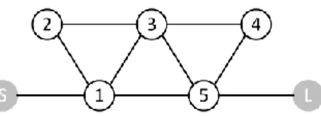
Fig. 2. Coupling topology of a five-pole filter with three TZs.
for RAT. In this work, a physics-based preconditioner for the start system is proposed.
It is very common in practice that an irregular coupling topology composed of a part with regular coupling topology and some additional weak irregular cross couplings. Physically, the filter response is dominated by the regular part whereas the intentionally introduced irregular cross couplings serve as “the icing on the cake”. Therefore, the coupling matrix in the regular topology that aligns with the physical solution can be first reconfigured deterministically to construct a preconditioner of the start system. It will be shown through numerical examples that such a preconditioner can very well serve as the start system which effectively leads to the correct solution through the homotopy continuation process. When unintentional irregular cross couplings have to be introduced due to stray couplings, the solution corresponding to the part with regular coupling topology can be obtained by ignoring the far away TZs, leading to a physical preconditioner.
In dealing with an irregular coupling topology with multiple irregular cross couplings, in order to avoid multiple solution problem, a bootstrapping approach can be taken, by which the homotopy continuation process is applied multiple times with a progressive increase of irregular cross couplings. The details will be illustrated in the third example in the next section.
Note that this method is based on the hypothesis that the irregular coupling topology has a real solution for any lossless responses that comply with the shortest path rule [16]. If the irregular cross coupling is poorly located, there is a conceptual possibility that the topology has no physical solution. Nevertheless, an appropriate topology can eventually be obtained by trial-and-error since the failure of convergence of the proposed method indicates the bad choice of topology.
III. EXAMPLES AND CONVERGENCE OF SOLUTION
The proposed method is a general scheme not only for circuit model extraction problems but also for direct synthesis problems of bandpass filters with irregular topologies. The first illustrative example will be a synthesis problem of a 5-pole filter with an intentional irregular cross coupling, through which every detail of establishing a homotopy and the continuation process will be given. The second example is a practical 10-pole filter in a regular topology yet with an extra parasitic cross coupling, with which the accuracy of the method is demonstrated. The last example demonstrates how the proposed method is used in a RAT process of a 10-pole filter with more than one irregular couplings, in which the bootstrapping approach is applied.
The synthesis of a five-pole filter that generates 3 TZs in the topology depicted in Fig. 2 is considered. Two of the three TZs are placed at −1.6j and 2.4j in the normalized lowpass frequency domain, which can be easily realized by two CTs. It’s convenient to add a cross coupling between resonators 1 and 5 to create the third TZ at −8j to enhance the rejection in the far lower rejection band. For such a coupling topology there is no known rotation recipe for reconfiguration.
With the given TZs and specified 20 dB return loss level, the coupling matrix in the folded canonical form can be easily obtained and is denoted as MC. The first step to reconfigure MC
to the coupling matrix, say M0, in the desired topology is to
establish a polynomial equation system. Basically, the orthogonal transformation matrix Q can be set as a blockwise diagonal matrix diag (1, Qx, 1) with Qx being an N × N block matrix whose elements are unknown [7]. However, the set of the unknowns can usually be reduced to a less-redundant one by reducing the dimension of Qx such that Q = diag (I, Qx, I) in a trial-and-error way with symbolic calculation. In this example, the orthogonal transformation matrix Q can be set in the form of 1 2 3 4 5 6 7 8 9 1 0 0 0 0 0 0 0 1 0 0 0 0 0 0 0 0 0 0 0 0 0 0 0 0 0 0 0 0 0 0 1 0 0 0 0 0 0 0 1 x x x x x x x x x Q (12)
where the unknown vector is x = [x1, x2, …, x9]. Comparing QTM
CQ against the desired coupling topology, the homotopy
function H is formulated according to (2) as
3 3 4 1 3 5 3 4 12 3 7 5 1 6 6 4 6 7 6 7 7 4 9 12 1 9 8 7 9 13 1 9 7 1 2 4 5 7 8 1 3 4 6 7 9 2 3 5 6 8 9 2 2 2 1 4 7 2 2 2 2 5 8 2 2 2 3 6 9 0 0 0 0 0 0 1 0 1 0 1 0 a x a x x a x x a x x a x x a x x a x x a x x a x x x x x x x x x a x x a x a x x x x x x x H x x x x x x x x x x x x x x (13) with a = t m1 + (1 - t) m0 and m = [Ms,1, M1,1, M1,2, M2,2, M2,3, M3,3, M3,4, M4,4, M4,5, M5,5, M5,L, M2,4, M2,5, M1,5]. Subsequently,
the Jacobian matrices with respect to x and t can be found according to (4) and (5).
Assume the TZs 2.4j and −1.6j are assigned to CT (1-2-3) and CT (3-4-5), respectively. Then a physics-based approximation for M1 is chosen to be the coupling matrix in the
coupling topology without cross coupling M1,5, which can be
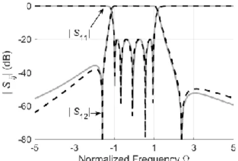
Fig. 3. Response of the start system M1 (solid lines) and the target system
M0 (dashed lines) of the 5-pole filter.
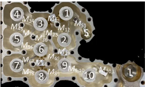
Fig. 4. A clipped photo of the coaxial combline filter (for example B) in a mult-filter module for 5G applications.
Fig. 5. Topology of the ten-pole filter in Fig. 4 with one CT, two CQs, and a parasitic coupling represented in the dashed line.
1 0 1.0076 0 0 0 0 0 1.0076 0.0105 0.8186 0.2407 0 0 0 0 0.8186 0.3641 0.5986 0 0 0 0 0.2407 0.5986 0.0288 0.5411 0.3899 0 0 0 0 0.5411 0.5466 0.7590 0 0 0 0 0.3899 0.7590 0.0105 1.0076 0 0 0 0 0 1.0076 0 M
By transforming M1 to the folded form by a deterministic
process as 1 0 1.0076 0 0 0 0 0 1.0076 0.0105 0.8533 0 0 0 0 0 0.8533 0.0134 0.6004 0.1257 0.1100 0 0 0 0.6004 0.2132 0.6834 0 0 0 0 0.1257 0.6834 0.0461 0.8462 0 0 0 0.1100 0 0.8462 0.0105 1.0076 0 0 0 0 0 1.0076 0 C M
one can find the preconditioner Q for the start system, or
1 0.9594 0.2821 0 0.2530 0.8606 0.4421 0.1247 0.4241 0.8907
T
x
with parameterm1 composed by coupling coefficients in MC1.
Note that this is a degenerate system since it satisfies the polynomial equation system without cross coupling M1,5. The
filter response of M1 is shown in Fig. 3 in solid lines. The
coupling matrix MC0 for the system with cross coupling M1,5 in
folded form can be easily found by the traditional synthesis method as 0 0 1.0079 0 0 0 0 0 1.0079 0.0139 0.8539 0 0 0.0118 0 0 0.8539 0.0159 0.5959 0.1798 0.0961 0 0 0 0.5959 0.2956 0.6627 0 0 0 0 0.1798 0.6627 0.0566 0.8484 0 0 0.0118 0.0961 0 0.8484 0.0139 1.0079 0 0 0 0 0 1.0079 0 C M
and consequently, the parameter m0,which represents the target
system to solve.
With the homotopy function and the preconditioner x1 for the
start system, the solution for the target system m0 can be found
by the coefficient-parameter homotopy continuation method as
0 0.9726 0.2325 0 0.2047 0.8563 0.4741 0.1102 0.4611 0.8805
T
x
with which the synthesized coupling matrix M0 is found as
0 0 1.0079 0 0 0 0 0 1.0076 0.0139 0.8305 0.1985 0 0.0118 0 0 0.8305 0.3074 0.6134 0 0 0 0 0.1985 0.6134 0.0453 0.5262 0.4136 0 0 0 0 0.5262 0.5759 0.7470 0 0 0.0118 0 0.4136 0.7470 0.0139 1.0079 0 0 0 0 0 1.0079 0 M
whose filter response is shown in Fig. 3 in dashed lines. As expected, higher rejection in the lower rejection band is obtained. By perturbing M2,2 and M4,4 in M0 separately, it is
confirmed that TZs corresponding to CT (1-2-3) and CT (3-4-5) are the same as those initially assigned, validating that M0 is the
correct solution.
It is interesting to look at the preconditioner from multiple solution point of view. By using a tool like Dedale-HF [8] one can compute all solutions associated to the irregular topology in Fig. 2. It is found that the total number (not counting the classical sign changes), which is the reduced order of the
topology [7], of solutions in this example is 2. When the third transmission zero at -8j is progressively sent to infinity, the two solutions converge to the two solutions corresponding to the two possible assignments of TZs to the two triplets. This explanation justifies the correspondence between the physics-based preconditioner in a regular coupling topology and the final solution in an irregular coupling topology. In other words, provided that the third TZ is sufficiently far away from the passband, the knowledge of the regular part of the coupling matrix can be used as a preconditioner to uniquely determine the final coupling matrix via the continuation process. B. A 10-Pole Filter in Regular Topology with a Parasitic TZ
This example intends to demonstrate the effectiveness of the method in extracting the coupling matrix from the measured filter response. A coaxial combline filter in a multi-filter module that consists of 16 similar filters for a 5G base station product is shown in Fig. 4, the coupling topology of which shown in Fig. 5 contains one CT and two CQs in its physical realization. A parasitic coupling that is supposedly caused by the stray coupling between resonator 7 and the load, or M7, L, is
also presented in Fig. 5 in a dashed line. This parasitic coupling is chosen based on the shortest path rule [16] to accommodate
COUPLING MATRIX MC0 OF EXAMPLE B MS1 M12 M23 M34 M45 M56 1.0406 -0.0029j 0.7662 -0.0005j 0.6148 +0.0002j 0.5440 -0.0004j 0.3990 0.5681 -0.0004j M67 M78 M89 M9,10 M10,L M57 0.1916 +0.0005j 0.5050 -0.0008j 0.7218 +0.0001j 0.8559 -0.0003j 1.0426 -0.0018j 0.0566 +0.0008j M47 M48 M38 M39 M29 -0.5232 0.1237 +0.0008j 0.0844 -0.0312 -0.0003j -0.0009 +0.0001j MSS M11 M22 M33 M44 M55 -0.0016 -0.0142j 0.4309 -0.0134j -0.5044 -0.0073j -0.2215 -0.0069j -0.4212 -0.0075j -0.1097 -0.0073j M66 M77 M88 M99 M10,10 MLL 0.6160 -0.0082j 0.1665 -0.0061j -0.0512 -0.0068j 0.0358 -0.0074j 0.0152 -0.0196j 0.0043 -0.0218j TABLE III
COUPLING MATRIX M0 OF EXAMPLE B
MS1 M12 M14 M23 M24 M34 1.0406 -0.0029j 0.6601 -0.0009j 0.3889 +0.0005j 0.1533 +0.0002j 0.4080 -0.0007j 0.2240 M45 M46 M56 M67 M78 M79 0.5381 +0.0002j -0.1633 +0.0005j 0.4533 -0.0001j 0.5410 -0.0006j 0.2607 -0.0015j -0.4610 +0.0024j M7,10 M7L M89 M9,10 M10,L 0.3834 +0.0027j 0.0170 -0.0011j 0.1785 -0.0016j 0.7751 -0.0024j 1.0425 -0.0018j MSS M11 M22 M33 M44 M55 -0.0016 -0.0142j 0.4309 -0.0134j -1.0311 -0.0082j -0.3959 -0.0069j -0.3722 -0.0069j 0.1547 -0.0083j M66 M77 M88 M99 M10,10 MLL -0.0757 -0.0081j -0.2720 -0.0104j 0.9430 -0.0066j 0.5717 -0.0028j 0.0028 -0.0189j 0.0043 -0.0218j
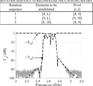
ROTATION SEQUENCE TO RECONFIGURE THE COUPLING MATRIX Rotation sequence Elements to be annihilated Pivot [i, j] 1 [8, L] [8, 9] 2 [9, L] [9, 10] 3 [8, 10] [8, 9]
Fig. 6. Measured response (solid line) and the recovered response (dashed line) corresponding to M0 without the imaginary parts of inter-resonator
couplings.
the parasitic TZ mathematically. The center frequency of the filter f0 = 2.591 GHz and the bandwidth BW = 194 MHz.
In this example, the polynomials for the filtering function are identified from the measured S-parameters using MVF with an extra TZ. With the polynomials, MC0 in the folded form can be
easily obtained and is listed in Table II, with which the required polynomial homotopy system can be built according to (1).
It can be easily found by perturbation that the desired TZ at -1.865 j is realized by CT (4-5-6); TZ pair at (1.136j, +1.237j) are controlled by CQ (1-2-3-4); and TZ pair at (-1.108j, -1.261j) are controlled by CQ (7-8-9-10). The coupling matrix M1 in
coupling topology without M7, L can be easily synthesized with
20 dB return loss in the specified passband. The solution x1 for
the start system can be obtained by transforming M1 to MC1,
which is in canonical form according to (10). Note that such a start system is a degenerate system since M1 is not exactly in
the desired coupling topology. However, the degenerate system can be found efficiently and can serve as a very good preconditioner.
The coupling matrix MC0 in canonical form is used as the
parameters for the target system in the desired topology. By following the procedure given in Table I and using the preconditioner as the start system, the target system M0 in the
coupling topology of Fig. 5 can be obtained aslisted in Table III, in which the imaginary part of the self-coupling terms represents the loss. Due to numerical errors in MVF caused by measurement noise and non-physical locations of spurious couplings to a certain extent, a very small amount of imaginary parts may occur in off-diagonal terms. Such small imaginary parts can be omitted without visibly affecting the response. As presented in Fig. 6, the filter response obtained by the reconfigured M0 with the imaginary parts of inter-resonator
couplings neglected matches the measured response very well. In fact, a direct annihilating rotation sequence can be found for this special irregular coupling topology. After the conventional reconfiguration process for obtaining CQ (1-2-3-4) and CT (4-5-6), the final coupling matrix can be reconfigured by 3 more sequentially rotations, as listed in Table IV, for annihilating M8,L, M9,L, and M8,10, resulting in exactly the same
coupling matrix as M0 obtained by the homotopy continuation
method. This fact further verifies the proposed preconditioner and the numerical continuation process.
Actually, the existence of coupling M7,L changes the CQ
closest to the load port to a quintet in arrow form, which is also a canonical block with a unique solution. Therefore, the degenerate system M1 will evolve to the unique solution if the
assignment of TZs to each cascaded block in M1 is the same as
that of M0. In fact, there is a one-to-one mapping in solutions
between the irregular topology and any other topologies with which the missing cross coupling down the minimum path causes one TZ to vanish consequently. For RAT applications, this feature means that if a regular part of the coupling topology can be clearly identified the coupling matrix for the irregular topology will converge to the unique solution with the preconditioner.
The parasitic coupling M7,L is artificially introduced to the
circuit to accommodate the unintentional TZ. It’s observed that the coupling value is relatively small and stable during the tuning process. A new golden template matrix is subsequently
Fig. 7. A clipped photo of the coaxial combline filter (for example C) in a multi-filter module for 5G applications.
Fig. 8. Topology of a ten-pole filter in Fig. 7 with an irregular cross coupling and a parasitic coupling represented in the dashed line.
Fig. 9. Response of the preconditioner (solid lines) corresponding to M1 and
the synthesized golden template (dashed lines) corresponding to M0 of
example C.
TABLE V
COUPLING MATRIX M0 FOR THE GOLDEN TEMPLATE MATRIX OF EXAMPLE C
S 1 2 3 4 5 6 7 8 9 10 L S 0 0.9809 0 0 0 0 0 0 0 0 0 0 1 0.9809 0 0.7999 -0.0937 0 0 0 0 0 0 0 0 2 0 0.7999 0.1344 0.5723 0 0 0 0 0 -0.0034 0 0 3 0 -0.0937 0.5723 -0.0179 0.2317 0.4392 0.2075 0 0 0 0 0 4 0 0 0 0.2317 -0.9201 0.1449 0 0 0 0 0 0 5 0 0 0 0.4392 0.1449 -0.3598 0.4843 0 0 0 0 0 6 0 0 0 0.2075 0 0.4843 -0.018 0.2376 -0.4298 0.217 0 0 7 0 0 0 0 0 0 0.2376 0.9064 0.1669 0 0 0 8 0 0 0 0 0 0 -0.4298 0.1669 0.3512 0.5355 0 0 9 0 0 -0.0034 0 0 0 0.217 0 0.5355 0 0.8053 0 10 0 0 0 0 0 0 0 0 0 0.8053 0 0.9809 L 0 0 0 0 0 0 0 0 0 0 0.9809 0
generated by incorporating the parasitic TZ. Then, the tuning process can be properly guided with the updated target coupling matrix.
C. A 10-Pole Filter with both Intentional and Unintentional Irregular Couplings
Another 10-pole filter is studied in this example, whose physical layout is shown in Fig. 7. This example will illustrate
that the coefficient-parameter homotopy continuation can be efficiently applied to model extraction of a high order filter which is with both intentional and unintentional irregular couplings.
As illustrated in Fig. 8, the coupling topology consists of an intentional irregular cross coupling M2,9 on top of the regular
one CT and two CQs topology, as well as a parasitic coupling M2,10, which needs to be introduced to accommodate a parasitic
TZ. Coupling M2,9 is introduced conveniently to create an extra
TZ to further suppress the rejection since resonators 2 and 9 are physically adjacent.
The extraction process will take two steps in a bootstrapping manner:
Step 1: a golden template coupling matrix that corresponds to the physical layout without considering the parasitic coupling M2,10, is synthesized using the proposed preconditioner and the
continuation method. Assigning a TZ at -1.816j to CT(1-2-3), a pair of TZs (1.128j, 1.253j) to CQ(3-4-5-6), and a pair of TZs (-1.134j, -1.385j) to CQ(6-7-8-9), the preconditioner M1 for
synthesizing the template can be obtained based on the regular part of the filter layout without M2,9, and M2,10 of course. The
coupling matrix MC0 in folded form for the system with the
additional TZ at about 3.5j due to cross coupling M2,9 can be
easily found by the traditional synthesis method. The synthesized response is equal-ripple in the passband. Similar to example A in this Section, the template coupling matrix M0
corresponding to the physical layout can be obtained using the coefficient-parameter homotopy continuation, which is listed in Table V. The responses of the golden template matrix M0 (in
dashed lines) is compared to that of the preconditioner of M1 (in
solid lines) in Fig. 9. It is observed that with M2,9 introduced,
the suppression in the higher rejection band is increased. Step 2: To accommodate the parasitic coupling M2,10, which
is identified from the parasitic TZ in the measured response of the real filter, the golden template matrix M0 is used as the
preconditioner for reconfiguring the final coupling matrix from the measured data. Obviously, the final coupling matrix involves M2,9 and M2,10. Since the additional TZ introduced by
M2,10 on top of those of the preconditioner is far away from the
passband, applying the homotopy continuation process will lead to a unique solution. The bootstrapping approach can be applied to other reconfiguration problems, in which more than one irregular couplings exist.
(a)
(b)
(c)
(d)
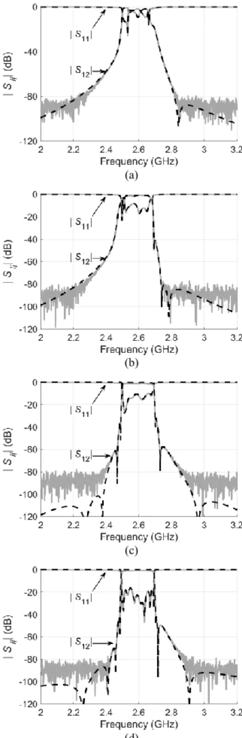
Fig. 10. Measured data in solid lines and responses by MVF in dashed lines of four tuning stages.
Step 2 can be applied to different tuning stages of a RAT process. Responses of reconfigured coupling matrices and the measured data of four typical tuning stages of the filter are superimposed in Figs. 10(a) - 10(d), showing excellent pertinence of the extracted coupling matrix in each stage. Note that the golden template matrix needs to be constantly updated by taking into account the parasitic coupling in the tuning process.
It is this proposed reconfiguration method that enables a progressively automatic tuning process in a deterministic fashion. The reconfigured coupling matrices in the four tuning stages are listed in Table VI. The elapsed time for reconfiguration of each tuning stage using the proposed method
with tens of iterations is about 0.75 seconds on average by a MATLAB [17] code on a PC computer.
IV. CONCLUSION
In this paper, an effective and efficient numerical approach for coupling matrix reconfiguration is proposed by introducing a legitimate and physics-based preconditioner in the parameter-coefficient continuation process. The preconditioner can greatly facilitate the continuation process to most of the practical filter problems, which involve irregular coupling topologies. By introducing the preconditioner, which can be easily obtained using classical filter synthesis theory, for the start system, the continuation process will lead to the unique solution corresponding to the given physical realization. The proposed approach is particularly useful not only for robot automatic tuning (RAT) but also for synthesizing advanced bandpass filters with irregular couplings, which are introduced either intentionally or unintentionally. The effectiveness and efficiency of the proposed approach have been validated and demonstrated through three practical examples, including a synthesis example, an extraction example, and a RAT of a 10-pole filter with 7 TZs. It is amazingly seen that the preconditioner can serve as a start system of the continuation
REAL PARTS OF COUPLING MATRICES OF THE FOUR TUNING STAGES IN FIGS.10(A)-(D)
Stage 1 Stage 2 Stage 3 Stage 4
MSS -0.0009 -0.0014 -0.0012 -0.0014 M11 -0.0259 -0.0219 0.0017 0.0171 M22 -0.0341 0.2967 0.2768 0.3683 M33 0.1567 0.1242 -0.0526 -0.0420 M44 -0.6493 -0.8493 -0.9499 -0.9607 M55 0.1318 -0.2775 -0.4011 -0.4142 M66 -0.2617 0.0865 -0.0210 -0.0134 M77 0.5715 0.8695 0.9461 0.9337 M88 0.3370 0.6802 0.4027 0.3700 M99 0.0136 0.0120 0.0135 0.0108 M10,10 0.0492 0.0547 0.0044 0.0204 MLL 0.0025 0.0071 -0.0074 0.0132 MS1 1.0594 1.0592 1.0589 1.0586 M12 0.7882 0.8326 0.8431 0.8430 M23 0.5091 0.5034 0.5410 0.5740 M34 0.2235 0.2187 0.2149 0.2165 M45 0.1680 0.1654 0.1652 0.1265 M56 0.3889 0.4249 0.4253 0.4854 M67 0.1913 0.1833 0.1953 0.2387 M78 0.1760 0.1802 0.1693 0.1677 M89 0.5581 0.5708 0.5538 0.5537 M9,10 0.8971 0.8967 0.8980 0.8564 M10,L 1.0069 1.0068 1.0047 1.0167 M13 -0.2369 -0.2362 -0.2043 -0.2209 M35 0.4497 0.4525 0.4559 0.4523 M36 0.1859 0.1958 0.1833 0.2304 M68 -0.4780 -0.4787 -0.4708 -0.4533 M69 0.2580 0.2431 0.2717 0.2330 M29 -0.0116 -0.0107 -0.0027 -0.0035 M2,10 -0.0007 -0.0007 0.0009 0.0009
process very robustly. It is believed that the approach can play an important role in future RAT of advanced microwave bandpass filters.
REFERENCES
[1] R. J. Cameron, “General coupling matrix synthesis methods for Chebyshev filtering functions,” IEEE Trans. Microw. Theory Tech., vol. 47, no. 4, pp. 433–442, Apr. 1999.
[2] H. Hu and K.-L. Wu, “A generalized coupling matrix extraction technique for bandpass filters with uneven-Qs,” IEEE Trans. Microw.
Theory Techn., vol. 62, no. 2, pp. 244–251, Feb. 2014.
[3] P. Zhao and K.-L. Wu, “Model-based vector-fitting method for circuit model extraction of coupled-resonator diplexers,” IEEE Trans. Microw.
Theory Techn., vol. 64, no. 6, pp. 1787–1797, Jun. 2016.
[4] R. J. Cameron, C. M. Kudsia, and R. Mansour, Microwave Filters for
Communication Systems: Fundamentals Design and Applications, 2nd ed. Hoboken, NJ, USA: Wiley, 2018.
[5] S. Tamiazzo and G. Macchiarella,“An analytical technique for the synthesis of cascaded N-tuplets cross-coupled resonators microwave filters using matrix rotations,” IEEE Trans. Microw. Theory Tech., vol. 53, no. 5, pp. 1693–1698, May 2005.
[6] B. S. Senior, I. C. Hunter, V. Postoyalko, R. Parry, "Optimum network topologies for high power microwave filters", 6th High Freq.
Postgraduate Student Colloq., 2001, pp. 53-58.
[7] R. J. Cameron, J. -C. Faugere, F. Rouillier, and F. Seyfert, “An exhaustive approach to the coupling matrix synthesis problem application to the design of high degree asymmetric filters,” Int. J. RF, Microw.
Computer-Aided Eng., vol. 17, no. 1, pp. 4–12, Jan. 2007.
[8] F. Seyfert, Dedale-HF. INRIA, Sophia-Antipolis, France, 2006. [Online]. Available: www-sop.inria.fr/apics/Dedale/.
[9] G. Macchiarella, “A powerful tool for the synthesis of prototype filters with arbitrary topology,” in IEEE MTT-S Int. Microw. Symp. Dig., July 2003, vol. 3, pp. 1467–1470.
[10] W. Atia, K. Zaki, and A. Atia, “Synthesis of general topology multiple coupled resonator filters by optimization,” in IEEE MTT-S Int. Microw.
Symp. Dig., Jun. 1998, vol. 2, pp. 821–824.
[11] S. Amari, “Synthesis of cross-coupled resonator filters using an analytical gradient-based optimization technique,” IEEE Trans. Microw. Theory
Techn., vol. 48, no. 9, pp. 1559–1564, Sep. 2000.
[12] M. Uhm, S. Nam, and J. Kim, “Synthesis of resonator filters with arbitrary topology using hybrid method,” IEEE Trans. Microw. Theory Techn., vol.55, no.10, pp. 2157–2167, Oct. 2007.
[13] S. Pflüger, C. Waldschmidt and V. Ziegler, “Coupling matrix extraction and reconfiguration using a generalized isospectral flow method,” IEEE
Trans. Microw. Theory Techn., vol. 64, no. 1, pp. 148–157, Jan. 2016.
[14] A. J, Sommese and , “Coefficient-parameter polynomial continuation,”
Appl. Math. Comput., vol. 29, pp. 123-160, Jan. 1989.
[15] A. J. Sommese and C. W. Wampler, The Numerical Solution of Systems of
Polynomials Arising in Engineering and Science, Singapore: World
Scientific. 2005.
[16] S. Amari, "On the maximum number of finite transmission zeros of coupled resonator filters with a given topology," in IEEE Microw. Guided
Wave Lett., vol. 9, no. 9, pp. 354-356, Sep. 1999.
[17] MATLAB, (R2019a), The Mathworks, Natick, Massachusetts, USA.
Yan Zhang (S’18) received the B.S.
degree in electronic engineering fromthe University of Electronic Science and Technology of China, Chengdu, China, in 2017. She is currently pursuing the Ph.D. degree at the Chinese University of Hong Kong, Shatin, Hong Kong. Her current research interests include synthesis and tuning of filters with dispersive couplings and filters with irregular topologies.
Ms. Zhang is a recipient of Hong Kong Ph.D. Fellowship.
Ke-Li Wu (M’90–SM’96–F’11) received
the B.S. and M.Eng. degrees from the Nanjing University of Science and Technology, Nanjing, China, in 1982 and 1985, respectively, and the Ph.D. degree from Laval University, Quebec, QC, Canada, in 1989. From 1989 to 1993, he was a Research Engineer with McMaster University, Canada. He joined COM DEV (now Honeywell Aerospace), Cambridge, ON Canada in 1993, where he was a Principal Member of Technical Staff. Since 1999, he has been with The Chinese University of Hong Kong, Hong Kong, where he is currently a Professor and the Director of the Radiofrequency Radiation Research Laboratory. His current research interests include EM-based circuit domain modeling of high-speed interconnections, robot automatic tuning of microwave filters, decoupling techniques of MIMO antennas, and IoT technologies. Prof. Wu is a member of the IEEE MTT-8 Subcommittee. He was a recipient of the 1998 COM DEV Achievement Award and the Asia-Pacific Microwave Conference Prize twice in 2008 and 2012, respectively. He was an Associate Editor of the IEEE Transactions on MTT from 2006 to 2009.
Fabien Seyfert graduated from the
“Ecole superieure des Mines” (Engineering School) in St Etienne (France) in 1993 and received his Ph.D. in mathematics in 1998. From 1998 to 2001 he joined Siemens (Munich, Germany) as a researcher specialized in discrete and continuous optimization methods. Since 2002 he occupies a full research position at INRIA (french agency for computer science and control, Nice, France). His research interest focuses on the conception of effective mathematical procedures and associated software for problems from signal processing including computer aided techniques for the design and tuning of microwave devices. In particular, he is the author of the software toolboxes Dedale-HF and Presto-HF.