HAL Id: hal-02419360
https://hal.archives-ouvertes.fr/hal-02419360
Submitted on 19 Dec 2019HAL is a multi-disciplinary open access
archive for the deposit and dissemination of sci-entific research documents, whether they are pub-lished or not. The documents may come from teaching and research institutions in France or abroad, or from public or private research centers.
L’archive ouverte pluridisciplinaire HAL, est destinée au dépôt et à la diffusion de documents scientifiques de niveau recherche, publiés ou non, émanant des établissements d’enseignement et de recherche français ou étrangers, des laboratoires publics ou privés.
Proposal for a protocol using an infrared
microbolometer camera and wavelet analysis to study
foot thermoregulation
Vincent Serantoni, Franck Jourdan, Hervé Louche, Ariane Sultan
To cite this version:
Vincent Serantoni, Franck Jourdan, Hervé Louche, Ariane Sultan. Proposal for a protocol using an infrared microbolometer camera and wavelet analysis to study foot thermoregulation. Quantitative InfraRed Thermography Journal, Taylor and Francis, In press, �10.1080/17686733.2019.1697847�. �hal-02419360�
1
Proposal for a protocol using an infrared microbolometer camera
and wavelet analysis to study foot thermoregulation
Vincent Serantoni(1), Franck Jourdan(1), Hervé Louche(1) and Ariane Sultan(2)
• Vincent Serantoni, Laboratoire de Mécanique et Génie Civil (LMGC), Université de Montpellier, CNRS, cc 048, place E. Bataillon, 34095 Montpellier Cedex, France, 04 67 14 96 34, [email protected]
• Franck Jourdan, Laboratoire de Mécanique et Génie Civil (LMGC), Université de Montpellier, CNRS, cc 048, place E. Bataillon, 34095 Montpellier Cedex, France, 04 67 14 96 34, [email protected]
• Corresponding author : Hervé Louche, Laboratoire de Mécanique et Génie Civil (LMGC), Université de Montpellier, CNRS, cc 048, place E. Bataillon, 34095 Montpellier Cedex, France, 04 67 14 96 34, [email protected] • Ariane Sultan, Equipe Nutrition Diabète, CHU Lapeyronie, 371, Av. Doyen G.
Giraud, 34295, Montpellier, Cedex 5, France, [email protected]
The research was conducted under the two affiliations (1) and (2)
Abstract
Here we propose a protocol to: (i) generate skin temperature (SkT) oscillations on glabrous tissues (plantar foot) in healthy subjects under controlled clinical environment conditions; (ii) measure quantitative temperature fields with an inexpensive microbolometer
2
(MB) infrared camera in a clinical environment; and (iii) quantify the characteristics of skin temperature (SkT) oscillations through spectral analysis.
We paid particular attention to the metrology of thermal measurements, with a special bench, including four homemade black body reference areas. We propose a live calibration procedure using this setup while correcting the thermal drift. After all of these correction steps, the experimental thermal resolution (𝑁𝐸𝑇𝐷𝑒𝑥𝑝) for the temporal variation in each
pixel was about 25 𝑚𝐾. Finally, a movement removal procedure was also applied to the
thermal images to avoid foot spatial movement over the 10 min observation period.
Thermoregulation was stimulated by a 6-min walking exercise test on six volunteers and was then studied using three kinds of scalar indicators evaluated before and after exercise per thermal image pixel.
We demonstrated that the 6-min walk exercise increased the thermoregulation activity beneath the plantar foot sole. Moreover, unlike manually placed local thermal probes, the indicator fields proposed in this paper allow the operator to select the exact thermoregulation activation locations and analyse the spatial distribution patterns at these locations.
Keywords: Wavelet analysis; skin temperature; thermoregulation; microbolometer infrared camera; thermal drift correction; motion correction
1. Introduction
Humans are well known to be homoeothermic and able to maintain a steady body temperature of about 37°C. Healthy people’s body temperature can range from 36.2 to 37.2°C according to a circadian rhythm[1]. This temperature remains relatively stable via many complex mechanisms and pathways, governed by thermoregulation. In extreme environmental conditions, the human body must rapidly cope with the problem of heat dissipation and heat generation to prevent any damage. The body temperature is basically kept stable by
3
with the environment through the skin. A clear link has long been established between SkBF and skin temperature (SkT). Comparisons between SkBF and SkT by different tests such as occlusion or cold stress have highlighted the efficacy of thermography for non-invasive measurement of SkBF[2]–[4]. Variations in SkBF, and thus in SkT, have been linked to specific thermoregulatory mechanisms. For example, Kastrup[5] demonstrated that oscillations with a frequency of around 0.04 Hz were linked to pure neurogenic activity. Finally, five frequency bands were identified (0.008-0.02 Hz, 0.02-0.05 Hz, 0.05-0.15 Hz, 0.15-0.4 Hz, and 0.4-2.0 Hz), respectively corresponding to endothelial, neurogenic, myogenic, respiratory, and cardiac origins [6]–[9]. The endothelial range corresponds to rhythmic regulation of vessel resistance initiated by metabolic substances released by endothelial cells. The neurogenic range corresponds to rythmic regulation of vessel size resulting from neurogenic activity. The myogenic range is attributed to the continuous response of smooth muscle cells to intravascular pressure changes. Finally, respiratory and cardiac ranges are linked to lung and heart activity.
Thermal oscillations induced by thermoregulation at the skin surface are dependent on many factors. As noted by Kenny et al.[10] in their review, reaching a specific mean body temperature threshold is one of the main conditions for thermoregulation activation. This threshold can be modified by aging or some pathologies such as diabetes mellitus. In healthy subjects, SkT thermoregulation oscillations can be impacted by this threshold and by other factors (environmental conditions, physical activity, disease, drug administration, etc.) able to modify body temperature. For example, administration of the vasodilatator acetylcholine (ACh) enhanced the oscillation amplitude at a frequency of 0.01 Hz [11]. Meanwhile, Parshakov[12] showed a decrease in thermoregulation amplitude in the neurogenic and endothelial frequency range in subjects with diabetic foot disease compared to a healthy group.
4
Various strategies such as drug administration[11], [13], occlusive reactions[14], [15], local cold stress[16], local heat stress[8], [12] and laser stimulation[17] have been proposed to activate and study thermoregulation mechanisms, and thus monitor SkT oscillations. The principle was to stimulate the skin near the location of probes used to measure SkT.
Nevertheless, as revealed by Jung[18] or Podtaev[9], local probes were used in many of these studies, which had two main disadvantages. The first one was the limitation to a small skin surface while the second was the marked variability in the results, depending highly on the probe location. Otherwise, infrared cameras offer the opportunity of monitoring physiological processes in real time and with high spatial resolution[19]. As human vessel structures differ between people, the use of a camera enables operators to specifically select the area of interest. Moreover, thermal images offer the opportunity to detect perforator vessels and highlight the large variability of spatial temperature distribution, even within a small area[20], [21]. These results led to the conclusion that probe registrations highly depend on the vessel network underlying the skin area in contact with the local thermal probe.
To our knowledge, few studies have focused on spectral analysis of thermoregulation activity on the basis of infrared images. Sagaidachnyi[22] used a thermal camera to
reconstruct and map thermal blood flow signals, but the application was not on
thermoregulatory quantification. Moreover, few articles concern spectral analysis of SkT thermoregulation oscillations, following a dedicated test to activate thermoregulatory
mechanism. Once these observations are obtained, it would be of interest to define a protocol for spectral thermal analysis of human thermoregulatory activity. The objective of the present study was to develop a protocol for studying thermoregulation disorders linked to some pathologies. An application to diabetic foot conditions will be the topic of a forthcoming paper.
5
Here we propose a protocol able to: (i) generate SkT oscillations in glabrous tissues (plantar foot), in healthy subjects, under controlled clinical environment conditions; (ii) measure quantitative temperature fields with an inexpensive infrared camera in a clinical environment; and (iii) quantify SkT oscillation characteristics through spectral analysis.
2. Materials and methods Experimental Protocol
One specific objective of the present study was to develop a thermal measurement protocol compatible with clinical environmental conditions for future applications to subjects with diabetic foot disease. It was therefore crucial to create a mobile, hygienic and easy to use procedure.
Because of the clinical environment and the scope of this study (quantify SkT oscillations), the thermal camera must satisfy all the following points: a small size (easy to carry and to place in a hospital room), high resolution (i.e. 640x480 px), thermal resolution below 50 mK, minimal frame rate of 5 Hz (necessary for future signal filtering) and no internal mechanical shutter. Moreover, it was crucial to have access to the raw digital values in order to perform all the corrections needed.
Considering all these criteria, an inexpensive microbolometer (MB) camera was thus chosen (Device-ALab, SmartIR640) and the entire following procedure was achieved contactless. Moreover, as indicated in the introduction, endothelial SkT oscillations associated with the thermoregulatory system are minor (often under 0.1°C), and very localised. So a high-sensitivity and -resolution thermal camera was therefore needed, and a homemade post-processing algorithm to treat each MB camera thermal image was formulated. The whole 3-step procedure is illustrated in Figure 1 and described in the next Metrology section.
6
As mentioned in the introduction, many thermoregulation activation protocols already exist, but many of them use local and contact activation systems. Without any external (through skin) or internal (exercises, etc.) stimulus, SkT is subject to various factors and can react differently. For example, as shown in the Figure 2, the temperature beneath the big toe of a volunteer (male, 49 years old) showed strong thermoregulation oscillations or a completely stable signal without any variations. This monitoring was carried out on different days, at different times during the day and under various room temperature conditions (𝑇!""#).
Oscillation activation was thus essential for thermoregulation quantification. For
thermoregulation activation, SkT was an important factor, but the body temperature seemed to be paramount. Thermoregulation was not activated if the body temperature was below a specific threshold[10]. Different protocols were tested in our laboratory to trigger
Figure 1: Experimental 3-step protocol to measure plantar foot temperature variations First and last image
(before and after correction)
Step1: removing fix pattern noise and
thermal drift effect from the raw signal
Step 2: time averaging and live
calibration for noise smoothing and thermal results.
Step 3: movement removal procedure
from the area of interest
Example of image correction (before and after step 1)
7
thermoregulation oscillations under the whole plantar foot sole. We tested different conditions: a warm plate beneath the feet, feet in warm water with direct or contralateral observations, cold spray beneath the feet and even use of a heating lamp. None of them were able to activate thermoregulation if the foot SkT was initially too low. Weakness of these tests was to increase only SkT without changing the body temperature. Exercise was the easiest way to raise the latter temperature. A new loading test, involving a 6-min walking exercise, gave good results in inducing thermoregulation oscillations. This is a well-known test exercise for assessing global responses of all systems involved during exercise. It implicates
pulmonary and cardiovascular systems, systemic circulation, peripheral circulation, blood circulation, neuromuscular units and muscle metabolism[23].
Finally, we propose the following experimental protocol. Subjects were monitored at least 2 h after breakfast or lunch. Once they arrived in the room, they were placed barefoot in a semi-Fowler’s position in a room at 25°C controlled temperature. The MB camera was placed in front of the foot sole (Figure 3). After 10 min of acclimation, the plantar foot sole temperature was recorded for 10 min to establish a baseline and they were asked to perform the 6-min walk test. Subjects’ heart rate was recorded before and after the exercise. It was assumed that
Figure 2: Temperature variations beneath the big toe of the same person (male) at different days under different room temperature conditions.
8
thermoregulation activation would occur during exercise or in the hyperaemia phase (post-exercise). Finally, the subjects were then recorded for a further 10 min, just after the exercise period. For computational simplicity, volunteers were asked to avoid any foot movement during all recording.
In each case, foot SkT oscillations were under interest. Wavelet analysis was used within a defined spectral range to quantify these variations.
Metrology
Quantitative thermoregulation studies require accurate tools. The MB camera chosen for the project had substantial drift according on its inner temperature, as well as relatively high noise. Moreover, the observed objects (feet) were moving slightly. In the following sections, we explain the procedure used to correct these artefacts and enhance the thermal image accuracy.
Box for neutral background during registration
Electrical resistance with PT100 probes
Infrared MB Camera Probe’s data recording for
live calibration
9
Step1: Non-uniformity correction and thermal drift correction
Some solutions have been proposed in the literature to manage and overcome fix pattern noise[24] and thermal drift effects of MB cameras.
Thermal images are always corrected via non-uniformity correction (NUC) to remove fixed pattern noise:
𝑈!"∗ 𝜙 = 𝐺
!!𝑈!" 𝜙 + 𝑂!" (1)
where 𝑈!" 𝜙 is the raw response measured by the detector (i,j), receiving a thermal flux; 𝜙. 𝑈!"∗ 𝜙 is the response after the NUC correction; 𝐺
!" and 𝑂!" are gain and offset correction
coefficients for each detector (i,j). These two coefficients are computed by: 𝐺!" =
𝑈 𝜙! − 𝑈(𝜙!)
𝑈!" 𝜙! − 𝑈!" 𝜙!
(2) 𝑂!" = 𝑈 𝜙! − 𝐺!"𝑈!" 𝜙! (3) where 𝑈!" 𝜙! and 𝑈!" 𝜙! are responses of a single detector (i,j) receiving radiation flux 𝜙! and 𝜙! coming from a black body at temperature 𝑇! and 𝑇! (with 𝑇! > 𝑇!). The terms 𝑈(𝜙!)
and 𝑈 𝜙! are mean values of all detectors. This correction is specific to each camera and effective only under a specific configuration (integration time and lens) and focal plane array temperature (FPAt).
When the latter changes, the detector electrical properties also change along with the output signal. The cooled kind of thermal camera is not very subject to this effect because a
dedicated part of the camera maintains the FPAt relatively stable over time. However, the MB camera FPAt constantly changes with the environmental conditions and due to self-heating. The output is thus strongly dependant on the FPAt, making accurate calibration impossible with a classical NUC. Figure 4b illustrates this point by showing the response (digital level - 𝑈!"∗) of three random detectors as a function of the FPAt. Recording was done after placing a
10
front of it, and recording detector variations over 1 h right after turning on the camera. Figure 4a shows the first frame of the recording. Substantial variation between detectors is clearly visible. As noted in Figure 4b, NUC was carried out with 𝑇!"#_!"# ≈ 42.7 °C, when all digital levels reached the same value. The detector signal responses vs FPAt showed a highly non-linear variation pattern. We observed a marked drop in the signal at low FPAt followed by a second more linear phase. After different tests, the marked drop was found to occur regardless of the initial FPAt. In each case, the second phase was observed around 15 min after turning on the camera. Therefore, it was assumed that this drop was probably the result of thermal inertia of the camera and all of its electronic components. In the presented case (Figure 4b), a FPAt deviation of 1°C from the initial value (𝑇!"#_!"#) led to a variation in the digital level from 42051 ± 37 (mean ± std) to 42301 ± 101. This variation changed the
thermal response by about 0.7 °C and drastically boosted the spatial noise.
Different methods have been proposed to correct the thermal drift. Nugent[25] corrected thermal drift by adding a linear part in the gain and offset definition, depending on the FPAt. Then, other studies such as Krupinski[26] and Budzier[27], corrected this drift effect with a dependence on the FPAt of only the offset, respectively with a linear or a polynomial relation. They assumed that the gain was not very affected by the FPAt and that an offset correction was enough. Our hypothesis in the present study was that, after the thermal inertia period, a linear correction of each detector could accurately correct the signal with regard to the drift effect. Based on Krupinski’s study, here we propose the following FPAt-dependent drift correction:
𝑈!" 𝜙 = 𝑈!"∗ 𝜙 + 𝐷𝐶𝐶
!"∙ 𝛿𝑇 (4)
where 𝑈!" 𝜙 is the output signal after NUC and drift correction; 𝑈!"∗ 𝜙 is the digital level
only after NUC correction, given by equation (1); 𝐷𝐶𝐶!" is the drift compensation coefficient of the detector (i,j) and 𝛿𝑇 = 𝑇!"# 𝑡 − 𝑇!"#_!"# is the FPAt deviation from its value after
11
NUC. An example of thermal drift correction is presented in the upper frame of the Erreur !
Source du renvoi introuvable..
Step 2: Time averaging and live calibration
The previous step enabled a stable response of all detectors regardless of the ambient temperature and FPAt. A calibration step is now mandatory to convert the digital level to temperature. A quantitative value, 𝑁𝐸𝑇𝐷!"#, was used to quantify the efficiency of the entire processing chain (NUC, thermal drift, time averaging and calibration). Indeed, the most common way to evaluate the smallest thermal variation that the detectors could detect was to use the noise equivalent temperature difference (NETD) defined by[28]:
𝑁𝐸𝑇𝐷 = 𝜎
𝑠𝑒𝑛𝑠𝑖𝑡𝑖𝑣𝑖𝑡𝑦 (5)
where 𝜎 is the mean temporal standard deviation of all detector digital levels, and sensitivity is the digital level to black body temperature change ratio. (in DL/°C). However, this
technique assumed a linearization of the calibration law around a chosen temperature. As discussed by Redjimi[29], an experimental NETD may be defined (different from the
Figure 4: a) Example of a digital level image of a black body set at a constant temperature (30°C); b) Digital level signal 𝑈!"∗, at points 1, 2 and 3 indicated in the left figure as a function of the FPAt.
𝑇𝐹𝑃𝐴_𝑁𝑈𝐶 represents the FPAt following NUC.
12
previous classic NETD) by taking the mean temporal standard deviation 𝜎 of all detectors after the calibration process. This 𝑁𝐸𝑇𝐷!"# will be used hereafter.
The most common calibration procedure involves finding coefficients of a polynomial function linking the digital level and temperature as:
𝑇!" = 𝑎!𝑈!"! + 𝑎
!!!𝑈!"!!!+ ⋯ + 𝑎!𝑈!" + 𝑎! (5)
where 𝑇!" is the thermal response of detector (i,j), 𝑎! represents the coefficients of the polynomial function and 𝑈!" is the digital level response of the detector (i,j), as described in eq. 4. For thermal images, it is generally accepted to use a 2nd or 3rd order polynomial function[30]. All coefficients are identified once in the laboratory, with a black body
evaluated at different temperatures. This technique is called fix calibration. Coefficients are constant and depend on a specific configuration (integration time and lens). As shown in Figure 5b, evaluation of the experimental NETD with the fix calibration technique led to 𝑁𝐸𝑇𝐷!"# ≈ 100 𝑚𝐾. This noise level was too high to study weak temperature variations due
to thermoregulation.
Figure 5: a) Thermal signal variations of a single detector recording a black body set at 30°C. Horizontal continuous and dotted lines are, respectively, the mean value and standard deviation; b) evaluation of the experimental NETD (standard deviation) from the data in the left figure.
13
We thus propose a better calibration based on live observations. On each image recorded by the camera, four different electrical resistances were also observed and acted as local black bodies. At steady state, these resistances (supply current: 1A) were at different constant temperatures (from ambient to about 35°C). Four PT100 probes (TE Connectivity, NB-PTCO-155, see close-up of Figure 3) were placed on these resistances, and the temperature was recorded at 1 Hz, synchronized with thermal acquisition. These resistances must be large enough in order to occupy, at least and for each, an area of 3x3 px in the field of view. Such an area is necessary to reduce the digital levels noise measured at the resistance surface. For each image, all coefficients of Eq.5 were computed (see Figure 1, step 2). With this technique, the experimental NETD decreased to 80 𝑚𝐾. This calibration is called live calibration
hereafter.
This thermal resolution was reduced to 40 𝑚𝐾 via time averaging (on five images). Then a last spatial averaging (Gaussian filter with standard deviation of 2 pixels) reduced the noise to a final 𝑁𝐸𝑇𝐷!"# = 25 𝑚𝐾. Step-by-step signal distribution variations are visible in Figure 6.
14
Step 3: Movement removal
During real thermal monitoring of plantar foot soles in a hospital, it was impossible to avoid all movements of both feet in the zone of interest (ZOI) over the 10 min recording period. A final post-processing step involved developing a tool able to remove movements from a selected ZOI. Such movement removal correction has widely been implemented in vision systems but few examples are available for thermal images [31].
The proposed tool required at least three input points. With the motion knowledge of these points, it was possible to correct movements throughout the ZOI. Therefore, for point 𝐼 moving across a space, the relation of the current position 𝑀′(𝑥!, 𝑦!) and its initial one 𝑀(𝑋!, 𝑌!) was: 𝑀! 𝑥 !, 𝑦! = 𝑥! = 𝑋! + 𝑢!(𝑋!, 𝑌!) 𝑦! = 𝑌! + 𝑢!(𝑋!, 𝑌!) (6) where 𝑢! and 𝑢! are the displacement components, in a Cartesian coordinate system (Figure 7). In order to identify the latter displacement parameters, a zero mean normalized cross-correlation (ZNCC) was used. This criterion is known to be insensitive to deformed image
Figure 6: Temperature variation response of a single random pixel recording a black body set at 30°C, a) histogram of thermal variations for the two kinds of calibration; b) histogram of thermal variations revealing the effect of spatiotemporal averaging. The respective experimental NETDs were 100 mK, 80 mK, 40 mK and 25 mK.
15
offset changes, and to be highly reliable[32]. A linear expression of 𝑢 was chosen to remove not only translation, but also rotation and distortion:
𝑢 𝑋!, 𝑌! = 𝑢𝑢! = 𝑎!+ 𝑎!𝑋! + 𝑎!𝑌!
! = 𝑏!+ 𝑏!𝑋!+ 𝑏!𝑌!
(7) where 𝑎! and 𝑏! (𝑘 = 0,1,2) are parameters identified through the following cost function
𝐹(𝑎!, 𝑏!):
𝐹 𝑎!, 𝑏! = [(𝑥!− (𝑋!+ !
𝑎!+ 𝑎!𝑋!+ 𝑎!𝑌!))!+ (𝑦!− (𝑌!+ 𝑏!+ 𝑏!𝑋!+ 𝑏!𝑌!))!] (8)
Because of the expression of 𝑢, a minimum of three different points were needed. After identification, it was possible to inverse equation (6) and remove all movements from each image compared to the first one. Only morphological information was used in this method. No external patterns (black paint or patches on the skin) were required. With this solution, it was possible to monitor each physiological part of the ZOI throughout the acquisition time without interacting physically with the subject. Hereafter thermal images will be plotted on the initial image of the recording. 𝑇!" = 𝑇!" 𝑡 = 𝑇(𝑋!, 𝑌!, 𝑡) is the notation for the temporal signal measured by the IR camera in pixels (i,j).
The signal recorded with the MB camera and processed through each step (1 to 3) was
accurate enough for quantitative physiological thermal investigation. The next part focuses on the tools used for spectral analysis of the latter signal.
16
Data processing
Wavelet processing tool
In the present study we aimed to quantify the thermoregulation activity. In many previous studies, wavelet analysis was preferred to classical Fourier analysis, which led to insufficient time resolution for nonstationary physiological signals[8], [33], [34]. However, a windowed Fourier transform was possible and could be used to achieve a good time-frequency analysis, but selection of a proper window size for good time and frequency resolution was impossible when there were complex signals, such as SkBF[7]. Therefore, despite the greater
computational complexity compared to Fourier transform, the continuous wavelet transform was preferred.
A so-called mother wavelet with a specific shape was used in the wavelet analysis. For physiological signals, the Morlet wavelet, i.e. a combined complex sinus and Gaussian function, is often chosen. The wavelet transform is defined as:
Figure 7 : Correlation illustration showing, for three points, the initial position M, the final position after displacement M’ and the displacement vector (blue) 𝑥⃗ 𝑦⃗
17
where 𝑊 𝑓, 𝑡 is the wavelet coefficient for different frequency 𝑓 and time 𝑡; 𝜓!,! 𝑢 is the
mother wavelet; 𝑇!" is the temporal signal in pixels (i,j); and [𝑡!, 𝑡!] is the time domain. This tool enables a good time-frequency resolution regardless of the signal as long as the edge effect (cone of influence) and Heisenberg's uncertainty principle are taken into account[35]. To maximally avoid edge effects, the most commonly used technique is to extend the signal by mirroring the latter at the start and end of the signal[36]. We used an odd mirroring technique in the present study.
To quantify the wavelet coefficient amplitude within a specific frequency range and time interval, the average amplitude was calculated using the following expression:
where 𝑊 is the mean amplitude of the wavelet coefficient in the range [𝑓!, 𝑓!], across time [𝑡!, 𝑡!].
Band-pass filtering
As mentioned in the introduction, frequencies of interest were in the interval [0.008 – 2 Hz]. Hence other frequencies need to be filtered, especially lower ones assigned to slow thermal motion, to ensure proper time-frequency analysis. A band-pass filter was thus designed and applied to each thermal signal, corresponding to the temperature recorded by each detector. The latter could be tuned for specific band-passes in the [0.008 – 2 Hz] range.
𝑊 𝑓, 𝑡 = 𝜓!,! 𝑢 𝑇!" 𝑢 𝑑𝑢 !! !! (9) 𝑊 = 1 𝑡!− 𝑡! 1 𝑓! − 𝑓! !! !! 𝑊 𝑓, 𝑡 𝑑𝑓𝑑𝑡 !! !! (10)
18
Finally, the evaluation of a signal recorded simultaneously by our MB camera and a cooled one revealed that spectral analysis was possible only in the endothelial and neurogenic range. This was done via phase coherence evaluation of both signals[16], [37].
It is important to note that, using a thermal camera with a good sensitivity, some correction steps may become unnecessary, but the test with the phase coherence evaluation is still mandatory. This test will indicate the frequency range where it is truly possible to distinguish the physiological signal from the electronic noise during the whole acquisition. If the result is good enough without a specific step, then this one is not mandatory anymore.
Analysis
Once each recording had passed through all the correction steps, the results were analysed using Matlab®. The developed processing tools allowed the operator to manually select a ZOI on the foot soles in order to extract different information, such as mean wavelet amplitude, standard deviation and mean temperature. The ZOI included the five metatarsal heads and the big toe. For each pixel (i,j) inside this ZOI, standard deviation (𝑠𝑡𝑑!") and maximal temperature variation (∆𝑇!" = max!∈ !!!" !"# (𝑇!" 𝑡 ) − min!∈ !!!" !"# (𝑇!" 𝑡 )) of the temporal temperature raw signals 𝑇!"(𝑡) were calculated. These scalar temporal indicators were then noted 𝑠𝑡𝑑!"!"#$, 𝑠𝑡𝑑
!"
!"#$%, ∆𝑇
!"!"#$ and ∆𝑇!"!"#$% when calculated on the temporal
temperature signal, filtered respectively in the endothelial and neurogenic frequency ranges. The mean wavelet amplitude indicator defined by Eq. 10 was calculated only in these two frequency ranges. They are denoted 𝑊!"!"#$ and 𝑊
!"!"#$%. All indicators computed in each
pixel (i,j) were mapped onto the whole ZOI in order to get indicator fields, denoted (𝒔𝒕𝒅, ∆𝑻 and 𝑾). An example of the field 𝑾𝒆𝒏𝒅𝒐 is given in Figure 8 for one subject. The spatial
distribution of this indicator was not uniform. This non-uniformity, enhancing the perforator vessel network, was observed for all other indicators. The point where the maximum of an indicator was observed (as shown by an arrow in Figure 8) was selected and considered as
19
being the most active point located in (𝑖!, 𝑗!) pixel position. The next section presents indicator values for each subject before and after exercise.
The effect of the 6-min walking exercise was finally studied using a non-parametric Kruskal-Wallis statistical test (𝛼 = 0.05).
Figure 8: mean wavelet amplitude indicator field (𝑾!𝒆𝒏𝒅𝒐 – in color), superimposed on a thermal image(in gray). 𝑖! 𝑗! Me an w av el et v al ue ( 10 ! ! °C )
20
3. Results
Six healthy volunteers were recruited (average age: 51.3 ± 5.3; two women, four men; body mass index (BMI): 70.7± 5.4) to assess the feasibility of the protocol. All volunteers were non-smokers and had no history of neurologic or ischemic disease.
Baseline vs post-exercise
The active point maximising any indicator was generally located on the same position on the foot sole. Temporal variations in the active point during the 10 min recording period
measured before and after exercise were respectively plotted in Figure 9 left and right. No distinction between the side of the limb (left or right foot) was done at this time in the presented results.
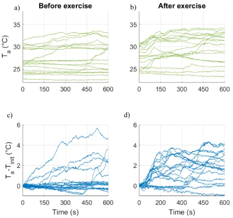
Figure 9: Temporal responses for all subjects of temperature at the active point (𝑖!, 𝑗!) before
exercise (a) and after (b). Thermal variation at the same point from the initial temperature before exercise (c) and after (d).
c) d)
21
The temperature responses before and after exercise differed. Scattering was greater before exercise than after. The temporal signals shown in Figure 9a and Figure 9b, with a low mean absolute temperature, were less active compare to those with a higher mean absolute
temperature. A thermal variation signal (𝑇!− 𝑇!"!#) was then computed, where 𝑇! =
𝑇(𝑋!!, 𝑌!!, 𝑡) is the temperature of the active point located in (𝑋!!, 𝑌!!) at current time 𝑡, and 𝑇!"!# is the initial temperature 𝑇(𝑋!!, 𝑌!!, 0) at this point. These signals, calculated for all
subjects (Figure 9c and d), showed that for some subjects no temperature variation was observed before exercise compared to post-exercise where almost all subjects exhibited temperature variations. These post-exercise variations oscillated between -1 and 4°C, instead of -1 to 5.5 °C before exercise.
Previous studies generally evaluated the foot mean temperature after 10-15 min with the subject remaining in a resting position[38], [39]. By averaging the temperature during the 9th min of recording before and after the exercise, a mean increase of 1.28 ± 0.74 °C was obtained for each volunteer.
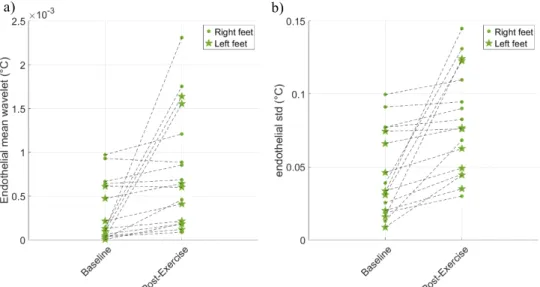
Variation patterns of all indicators, calculated in the active point (𝑋!!, 𝑌!!), were used to study the effect of exercise on thermoregulation activity. An example of the mean wavelet value in the endothelial range (𝑊!!"#$!!! ) and of the standard deviation in the same frequency range
(𝑠𝑡𝑑!!"#$!!! ) is illustrated in Figure 10. Indicators were computed for all subjects (left and right
foot) before and after exercise. These values increased after exercise, revealing a positive effect of the latter on thermoregulation activation.
The p-value of all the indicators chosen to study the effect of exercise are reported in Table 1. An increase in thermal activity was observed for all indicators (𝑝 < 0.011). Even if, in some cases, an oscillatory component already existed before exercise, the latter increased their amplitude during the following 10 min. The greatest effect was measured with the 𝑊!!"#$%!!! indicator.
22
Localization of the event
After mapping the wavelet results (𝑾), the active area was well contrasted from the rest of the ZOI and easy to detect. To characterize the localization of the active area, 𝑾𝒆𝒏𝒅𝒐 values were
studied in spatial directions. As shown in Figure 11a, two directions were chosen, one with a high drop (1) and the other with a slower drop (2). The results are plotted in Figure 11b. In direction (1), a 50% decrease was observed after 2.9 ± 0.51 𝑚𝑚 , whereas in direction (2) a similar drop was obtained after 5.8 ± 2.2 𝑚𝑚.
𝑠𝑡𝑑!!!! 𝑠𝑡𝑑!!"#$!!! 𝑠𝑡𝑑 !!!! !"#$% ∆𝑇 !!!! ∆𝑇!!!! !"#$ ∆𝑇 !!!! !"#$% 𝑊 !!!! !"#$ 𝑊 !!!! !"#$% p-value 0.0062 0.0045 0.0032 0.0049 0.0062 0.011 0.0056 0.00050 Table 1: Statistical results of the effect of the 6-min walk test carried out with a Kruskal-Wallis non-parametric test (α=0.05). a) b) Figure 10: Indicator variations for a healthy volunteer’s signal, filtered within the endothelial range. a) mean wavelet value 𝑊!!!!! !"#$, b) standard deviation 𝑠𝑡𝑑 !!!! !"#$. Dotted lines indicate, for each subject, variations in the indicator after exercise.
23
1 2
a) b)
Figure 11: a) 𝑾!!!𝒆𝒏𝒅𝒐field indicator plotted on the foot sole and selection of two directions of interest (1) and (2).
24
4. Discussion
As indicated by Kenny[10], the body temperature is a key factor for thermoregulation studies, as confirmed by our observations presented in Figure 2 and Figure 9a. A body temperature threshold must be reached to trig thermoregulation activity. Controlling or changing the body temperature in clinical environmental conditions and in pathologic (diabetic) patients is not easy. As noted in the introduction, some stimuli have been already proposed in the literature. Here we used an exercise test to raise the body temperature.
Our new protocol, involving a 6-min walk exercise, was assessed in this study. The findings of this study, carried out using an MB thermal camera and wavelet analysis, indicated that the 6-min walking exercise was able to activate thermoregulation on the whole plantar foot sole. Since our bench was unable to detect any temperature variations beyond 0.05 Hz, the study was limited to only endothelial and neurogenic frequency ranges. The latter was the most affected by the exercise (p<0.001), but all other indicators revealed an effect of the test.
Many previous studies focused on diabetic feet using thermal imaging revealed
marked activity beneath the big toe[40], [41], while in some of these studies only probes were used to compare SkBF and SkT. These probes were manually placed beneath the big toe. Mapping the results obtained on the foot sole enables precise localization of the active area. The results confirmed that for all subjects activation occurred under the big toe, and
sometimes under first or second metatarsal head (see Figure 11a). These areas of interest were placed so as to match with vascular network, especially with perforator vessels[42], [43] coming from the plantar metatarsal artery. However, as already indicated by Braverman[44] or Liu[21], our study revealed solid evidence of the necessity of the thermal imaging
technology, compared to the local technique. The exact location of the active area always depended on the subject. Moreover, it was found that a small gap of less than 5 𝑚𝑚 could change the value by up to 50%.
25
Study limitations were the weak activation achieved in different cases and the low number of subjects. This latter point will be improved in further studies in which more subjects will be involved, including diabetic patients. Finally, further studies are needed to precisely quantify the effect of the 6-min walking exercise on thermoregulation activation. Body temperature monitoring would help to accurately determine the activation threshold.
5. Conclusion
In this study we proposed a protocol to study thermoregulation oscillations. This protocol was able to: (i) generate SkT oscillations on glabrous tissues (plantar foot), in healthy subjects, in controlled clinical environment conditions; (ii) measure quantitative temperature fields with an inexpensive MB infrared camera in clinical environmental conditions; and (iii) quantify the characteristics of SkT oscillations through spectral analysis. One of the main constraints was to apply this protocol in a clinical environment where the setup cost was substantial.
Particular attention was paid to the thermal measurement metrology. A special bench, including four homemade black body reference areas, was designed and validated. Thanks to these reference areas, live calibration was carried out and the thermal drift was corrected. After all of these correction steps, the experimental thermal resolution (𝑁𝐸𝑇𝐷!"#) for
temporal variations per pixel was about 25 𝑚𝐾. Finally, a movement removal procedure was also applied to the thermal images to avoid foot spatial movement during the 10 min
observation period. Six healthy volunteers were chosen. Thermoregulation was stimulated by a 6-min walking exercise test and then studied using three kind of scalar indicators evaluated before and after exercise. The knowledge generated by these indicators, evaluated per pixel of the ZOI selected on the foot sole, allowed us to construct indicator fields that were plotted on the ZOI. Substantial localisation was observed in such fields, indicating areas concerned by
26
thermoregulation activity. Indicator values at the most active point were analysed for both feet in the six subjects.
The findings of this analysis demonstrated that thermoregulation activity on plantar foot sole was increased by the 6-min walk exercise. Moreover, unlike manually placed local thermal probes, the indicator fields that we used allow us to select the exact thermoregulation activation location, and to analyse the spatial distribution patterns of these locations.
Application of this protocol to patients with diabetic feet will be presented in a forthcoming paper.
6. Acknowledgment
This study was carried out thanks to the support of the LabEx NUMEV project (n° ANR-10-LABX-20) funded by the Investissements d’Avenir program managed by the French National Research Agency (ANR).
7. References
[1] K. Kräuchi, “How is the circadian rhythm of core body temperature regulated?,” Clin.
Auton. Res., vol. 12, pp. 147–149, 2002.
[2] J. E. Francis, “Thermography as a Means of Blood Perfusion Measurement,” J.
Biomech. Eng., vol. 101, p. 246, Apr. 2010.
[3] A. Lena Nilsson, “Blood Flow, Temperature, and Heat Loss of Skin Exposed to Local
Radiative and Convective Cooling,” J. Invest. Dermatol., vol. 88, pp. 586–593, 1987.
[4] S. B Wilson and V. Spence, “Dynamic thermographic imaging method for quantifying
dermal perfusion: potential and limitations,” Med. Biol. Eng. Comput., vol. 27, pp. 496–501, 1989.
[5] J. Kastrup, J. Bülow, and N. A Lassen, “Vasomotion in human skin before and after
local heating recorded with laser Doppler flowmetry. A method for induction of vasomotion,” Int. J. Microcirc. Clin. Exp., vol. 8, pp. 205–215, 1989.
[6] M. Bracic and A. Stefanovska, “Wavelet-based Analysis of Human Blood-flow
Dynamics,” Bull. Math. Biol., vol. 60, pp. 919–935, 1998.
27
peripheral blood circulation measured by laser Doppler technique,” IEEE Trans.
Biomed. Eng., vol. 46, pp. 1230–1239, 1999.
[8] M. Jo Geyer, Y.-K. Jan, D. Brienza, and M. L Boninger, “Using wavelet analysis to
characterize the thermoregulatory mechanisms of sacral skin blood flow,” J. Rehabil.
Res. Dev., vol. 41, pp. 797–806, 2004.
[9] S. Podtaev, M. Morozov, and P. Frick, “Wavelet-based Correlations of Skin
Temperature and Blood Flow Oscillations,” Cardiovasc. Eng., vol. 8, pp. 185–189, 2008.
[10] G. P. Kenny, R. Sigal, and R. McGinn, “Body temperature regulation in diabetes,”
Temperature, vol. 3, p. 0, 2016.
[11] H. Kvernmo, A. Stefanovska, K. Kirkebøen, and K. Kvernebo, “Oscillations in the Human Cutaneous Blood Perfusion Signal Modified by Endothelium-Dependent and Endothelium-Independent Vasodilators,” Microvasc. Res., vol. 57, pp. 298–309, 1999. [12] A. Parshakov, N. Zubareva, S. Podtaev, and P. Frick, “Local Heating Test for
Detection of Microcirculation Abnormalities in Patients with Diabetes-Related Foot Complications,” Adv. Skin Wound Care, vol. 30, pp. 158–166, 2017.
[13] P. Kvandal, S. Landsverk, A. Bernjak, A. Stefanovska, H. Kvernmo, and K. Kirkebøen, “Low-frequency oscillations of the laser Doppler perfusion signal in human skin,”
Microvasc. Res., vol. 72, pp. 120–127, 2006.
[14] A. Humeau-Heurtier, J. Louis Saumet, and J. Pierre L’Huillier, “Use of Wavelets to Accurately Determine Parameters of Laser Doppler Reactive Hyperemia,” Microvasc.
Res., vol. 60, pp. 141–148, 2000.
[15] A. Bagno and R. Martini, “Wavelet analysis of the Laser Doppler signal to assess skin perfusion,” 2015.
[16] A. Bandrivskyy, A. Bernjak, P. McClintock, and A. Stefanovska, “Wavelet Phase Coherence Analysis: Application to Skin Temperature and Blood Flow,” Cardiovasc.
Eng., vol. 4, pp. 89–93, 2004.
[17] S. Podtaev, A. Dumler, N. Muravyov, M. Myasnikov, and K. Tsiberkin, “Laser-induced skin temperature oscillations,” in Proceedings of SPIE - The International
Society for Optical Engineering, 2010, vol. 7376.
[18] F. Jung et al., “Laser Doppler flux measurement for the assessment of cutaneous microcirculatio--critical remarks,” Clin. Hemorheol. Microcirc., vol. 55, 2013.
[19] A. Merla et al., “Infrared functional imaging applied to Raynaud’s phenomenon,” Eng.
Med. Biol. Mag. IEEE, vol. 21, pp. 73–79, Apr. 2002.
[20] T. Binzoni, T. Leung, D. T Delpy, M. A. Fauci, and D. Rüfenacht, “Mapping human skeletal muscle perforator vessels using a quantum well infrared photodetector (QWIP) might explain the variability of LAIRS and LDF measurements,” Phys. Med. Biol., vol. 49, pp. N165-73, Apr. 2004.
[21] W.-M. Liu et al., “Reconstruction of Thermographic Signals to Map Perforator Vessels in Humans.,” Quant. Infrared Thermogr. J., vol. 9, no. 2, pp. 123–133, Jan. 2012. [22] A. Sagaidachnyi, A. Fomin, D. Usanov, and A. Skripal, “Thermography-based blood
28
Physiol. Meas., vol. 38, pp. 272–288, 2017.
[23] A. Thoracic Society, “Guidelines for the six-minute walk test,” Am. J. Respir. Crit.
Care Med., vol. 166, pp. 111–117, 2002.
[24] M. Schulz and L. Caldwell, “Nonuniformity correction and correctability of infrared focal plane arrays,” Infrared Phys. Technol., vol. 36, no. 4, pp. 763–777, 1995.
[25] P. W. Nugent, J. A. Shaw, and N. J. Pust, “Correcting for focal-plane-array temperature dependence in microbolometer infrared cameras lacking thermal stabilization,” Opt.
Eng., vol. 52, no. 6, pp. 1–8, 2013.
[26] M. Krupiński, G. Bieszczad, T. Sosnowski, H. Madura, and S. Gogler, “Non-Uniformity Correction in Microbolometer Array with Temperature Influence Compensation,” Metrol. Meas. Syst., vol. 21, 2014.
[27] H. Budzier and G. Gerlach, “Calibration of uncooled thermal infrared cameras,” J.
Sensors Sens. Syst., vol. 4, pp. 187–197, 2015.
[28] O. Riou, S. Berrebi, and P. Bremond, “Nonuniformity correction and thermal drift compensation of thermal infrared camera,” Proc. SPIE - Int. Soc. Opt. Eng., vol. 5405, 2004.
[29] A. Redjimi, D. Knezevic, K. Savic, N. Jovanovic, M. Simovic, and D. Vasiljevic, “Noise Equivalent Temperature Difference model for thermal imagers: calculation and analysis,” Sci. Tech. Rev., 2014.
[30] V. Honorat, S. Moreau, J. M. Muracciole, B. Wattrisse, and A. Chrysochoos, “Calorimetric analysis of polymer behaviour using a pixel calibration of an IRFPA camera,” Quant. InfraRed Thermogr. J., vol. 2, no. 2, pp. 153–172, 2005.
[31] M. Strakowska, R. Strąkowski, B. Wiecek, and M. Strzelecki, “Cross-correlation based movement correction method for biomedical dynamic infrared imaging,” 2012.
[32] B. Pan, H. Xie, and Z. Wang, “Equivalence of digital image correlation criteria for pattern matching,” Appl. Opt., vol. 49, pp. 5501–5509, 2010.
[33] A. Parshakov, N. Zubareva, S. Podtaev, and P. Frick, “Detection of Endothelial Dysfunction Using Skin Temperature Oscillations Analysis During Local Heating in Patients With Peripheral Arterial Disease,” Microcirculation, vol. 23, pp. 406–415, 2016.
[34] S. Podtaev, R. Stepanov, S. E, and E. Loran, “Wavelet-analysis of skin temperature oscillations during local heating for revealing endothelial dysfunction,” Microvasc.
Res., vol. 97C, pp. 109–114, 2014.
[35] C. Torrence and G. P. Compo, “A Practical Guide to Wavelet Analysis,” Bull. Am.
Meteorol. Soc., vol. 79, 1997.
[36] I. Simonovski and M. Boltezar, “The norms and variances of the Gabor, Morlet and general harmonic wavelet functions,” J. Sound Vib. - J SOUND VIB, vol. 264, pp. 545– 557, 2003.
[37] I. Mizeva, “Phase coherence of 0.1 Hz microvascular tone oscillations during the local heating,” IOP Conf. Ser. Mater. Sci. Eng., vol. 208, p. 12027, 2017.
29
“Infrared Dermal Thermometry for the High-Risk Diabetic Foot,” Phys. Ther., vol. 77, no. 2, pp. 169–175, Feb. 1997.
[39] N. Papanas, K. Papatheodorou, D. Papazoglou, C. Monastiriotis, and E. Maltezos, “Foot temperature in type 2 diabetic patients with or without peripheral neuropathy.,”
Exp. Clin. Endocrinol. Diabetes, vol. 117, no. 1, pp. 44–47, Jan. 2009.
[40] Y. Fujiwara, T. Inukai, Y. Aso, and Y. Takemura, “Thermographic measurement of skin temperature recovery time of extremities in patients with type 2 diabetes mellitus.,” Exp. Clin. Endocrinol. Diabetes, vol. 108, no. 7, pp. 463–469, 2000. [41] H. Zotter, R. Kerbl, S. Gallistl, H. Nitsche, and M. Borkenstein, “Rewarming index of
the lower leg assessed by infrared thermography in adolescents with Type I diabetes mellitus,” J. Pediatr. Endocrinol. Metab., vol. 16, no. 9, pp. 1257–1262, 2003. [42] J. M. Johnson, C. T. Minson, and D. L. Kellogg, “Cutaneous Vasodilator and
Vasoconstrictor Mechanisms in Temperature Regulation,” in Comprehensive
Physiology, American Cancer Society, 2014, pp. 33–89.
[43] C. Attinger, P. Cooper, and P. Blume, “Vascular anatomy of the foot and ankle,” Oper.
Tech. Plast. Reconstr. Surg., vol. 4, pp. 183–198, 1997.
[44] I. M. Braverman, “The Cutaneous Microcirculation,” J. Investig. Dermatology Symp.