Acoustic modelling of near borehole anolmalies via the generalised radon transform

(1)

Acoustic Modelling of Near Borehole Anomalies

via the Generalised Radon Transform

by

Richard Sven Patterson

B.S., University of California, Riverside (1986)

(Physics)

Submitted to the Department of Earth, Atmospheric, and Planetary

Sciences

in partial fulfillment of the requirements for the degree of

Master of Science

at the

MASSACHUSETTS INSTITUTE OF TECHNOLOGY

May 1992

©

Massachusetts Institute of Technology 1992

All rights reserved

Signature of Author ... ... ...

Department of Earth, Atmospheric, and Planetary Sciences

% May 8th, 1992

C ertified by ...-..

....

. .. .. ...

. . .. .. . .. .

M. Nafi Toks6z

Professor of Geophysics

Thesis Advisor

Accepted by ...

Thomas H. Jordan

Chairman

(2)

To my mother Shirley Merle,

who instilled in me the importance of a higher education regardless of my final objectives.

(3)

Acoustic Modelling of Near Borehole Anomalies via the

Generalised Radon Transform

by

Richard Sven Patterson

Submitted to the Department of Earth, Atmospheric, and Planetary Sciences on May 8th, 1992, in partial fulfillment of the

requirements for the degree of Master of Science

Abstract

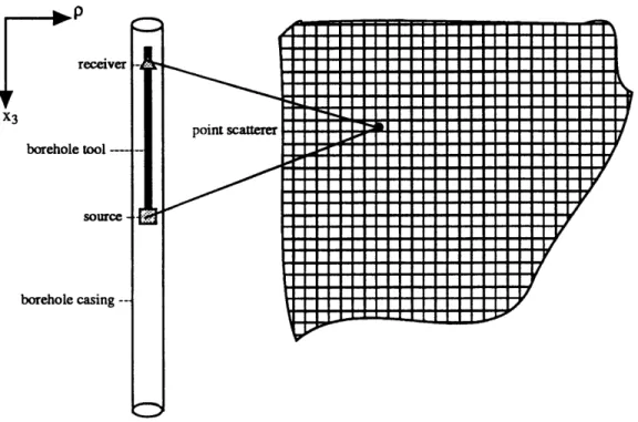
Data from well logging experiments are abundant in the oil exploration industry. This data is normally used to estimate borehole formation parameters. This thesis presents a theory and ensuing algorithm that will enable the exploration seismologist to image anomalies very near to the borehole (up to thirty wavelengths away from the borehole) using this data.

In this thesis we develop from first principles an analytical solution of the scat-tering wave equation in a 3D acoustic medium. The emerging inversion formula is analogous to a Generalised Radon Transform of the velocity structure of the medium over surfaces of constant travel time. If we assume that the scatterers are a com-posite of localised isolated perturbations of a constant velocity background medium, our inversion formula can be simplified to be analogous to a Radon transform of the velocity structure of the medium of interest. An inverse Radon transform is readily available and we apply this to obtain a simple expression for the scattering potential (a measure of the velocity perturbations) of the medium. We address the special data acquisition configuration of the Full Waveform Acoustic Logging (FWAL) tool and convert the inverse scattering equations into a form directly applicable to data collected by this seismic tool.

An algorithm based on our theory is applied to six synthetic 2D models. We ignore the effects of the borehole and any fluids they contain. For real data a re-scaling of the magnitude of the scattered data will have to be applied for our inversion technique to give satisfactory results. We address 2D models in this thesis, since data is cheaper to generate from these than their 3D counterparts. We argue that the very acoustic nature of our acquisition tool prohibits us from discerning the direction around the borehole from which the scattering occurs, and therefore any real 3D medium will appear to the FWAL tool as an infinite number of 2D slices along an axis of symmetry. Five of the six models analysed provide favourable results, which demonstrate

(4)

the feasibility of our algorithm in reconstructing point scatterers in very complex formations, dipping layers and beds, pinched-out layers often prevalent in fault zones, fractured regions and metamorphosised rocks. Our algorithm did not satisfactorily image inclusions and regions with velocity gradients.

In future work, we will apply the algorithm to real data from well logging ex-periments. We also hope to extend the theory presented in this thesis to an elastic medium.

Thesis Advisor: M. Nafi Toksdz Title: Professor of Geophysics

(5)

Acknowledgements

I would first like to thank Shawn Biehler, my undergraduate advisor at U.C.R, for encouraging me to go beyond a first degree and for his many words of praise that years later have kept me believing in myself even when I am at my lowest ebb.

I would also like to thank my present advisor, Nafi Toks5z, who has exhibited pa-tience even beyond Job, giving me second chances on too many occasions to mention.

My thanks also go out to the support staff at EAPS/ERL, especially Anita Killian,

Naida Buckingham and Liz Henderson. Thanks a million Liz for the editing for the final version.

My gratitude goes out to the people at ERL, especially Rick Gibson, Jeff Meredith,

Ningya Cheng, Ted Charrette and Bob Cicerone who have been there to answer my numerous questions, and to Sadi Kuleli who kept me "company" many a long night. To Steve Pride, a late but welcomed addition who has made several useful suggestions. Thanks also to Richard Coates for some guidance along the way. A separate note of thanks must go out to Joe Matarese who, more than anyone else, has always been there to help me and teach me aspects of geophysics, computers and beyond.

I am also grateful for a summer internship at ARCO where the work for this thesis commenced, especially to Ken Tubman and Robert Withers who suggested the topic for me to research.

To Wafik Beydoun who has so many times taken the time to share his vast theo-retical knowledge with me, when so many others were steering me towards the more practical aspects of geophysics; I would like to say thank you.

To my many friends who have made my stay away from. home more pleasant; in particular Roger Ally and Trevor Williams who gave vital support at many crucial times. I would like to say thank you.

To my family who have always been there for me, my heartfelt thanks go out to them. Especially to Daddy P.J., who rescued me from the well of despair too may times to mention.

(6)

To Lorraine who continually believes in me and has shown so much concern, making my problems her own; and for preventing me from making what probably would have been two of the biggest mistakes of my life, I would like to say thank you. To the Superior Being, whatever we may call him, for always looking out for me. I owe him everything.

(7)

List of Figures

2-1 A small section of the matrix of cells which make up the imaging re-gion as processed by this algorithm is shown along with the assumed borehole position. . . . .

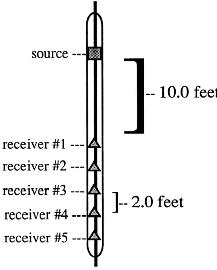
2-2 A scatterer located very close to the borehole and midway between the first and last source processed will view the source as having moved from -M to +M, with M being a very large number, during the course of the experiment. . . . . 3-1 This well logging tool has a source at the top of the tool and five evenly

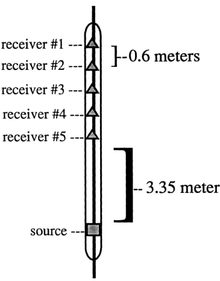
spaced receivers. . . . . 3-2 This well logging tool has a source at the bottom of the tool and five

3-3 3-4 3-5 3-6 3-7 3-8 3-9 3-10 3-11 3-12

evenly spaced receivers. . . . .

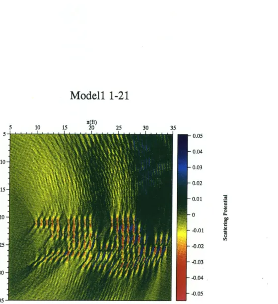
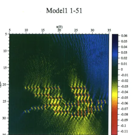
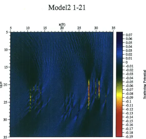
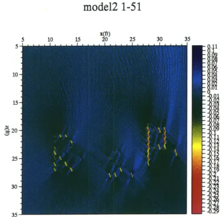
M odel 1 . . . . M odel 2 . . . . . M odel 3 . . . . Model4 ... Model5 ... M odel 6 . . . . Image of Model 1 using the first 21 sources. Image of Model 1 using all 51 sources. . . . Image of Model 2 using the first 21 sources. Image of Model 2 using all 51 sources. . . .

. . . . 60 . . . .. . 61 . . . .. . 62 . . . . 63 . . . .. . 64 . . . .. . 65 . . . . 66 . . . . 67 . . . . 68 . . . . 69 . . . . 70

(11)

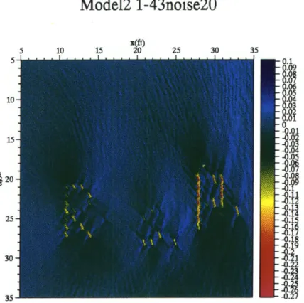
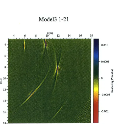
3-13 Image of Model 2 using the first 43 sources. Twenty percent of white noise has been added to the data before the imaging was performed. 71 3-14 Image of Model 3 using the first 21 sources. The scattering potential

has been rescaled to 0.01 of its true value. . . . . 72 3-15 Image of Model 3 using the first 51 sources. The scattering potential

has been rescaled to 0.01 of its true value. . . . . 73 3-16 Image of Model 3 using all 71 sources. The scattering potential has

been rescaled to 0.01 of its true value. . . . . 74 3-17 Image of Model 4 using the first 21 sources. The scattering potential

been rescaled to 0.01 of its true value. . . . . 77 3-20 Image of Model 5 using the first 51 sources. The scattering potential

has been rescaled to 0.01 of its true value. . . . . 78 3-21 Image of Model 5 using the first 51 sources. In this image we have

cho-sen an imaging region much closer to the borehole than in the two other images from this Model. The scattering potential has been rescaled to 0.01 of its true value. . . . . 79 3-22 Image of Model 5 using the first 71 sources. The scattering potential

(12)

3-25 Image of Model 6 using the first 51 sources. We have chosen an imaging region much further from the borehole than the previous two figures. The scattering potential has been rescaled to 0.01 of its true value. . 83 3-26 Image of Model 6 using all 71 sources. We have chosen an imaging

region much further from the borehole than that in the first two figures from this Model. The scattering potential has been rescaled to 0.01 of its true value. . . . . 84 3-27 Image of Model 6 using all 71 sources. We have chosen an imaging

region much closer to the borehole than that in the first two figures from this model. The scattering potential has been rescaled to 0.01 of its true value. . . . . 85 B-1 The contour -y is used to calculate, from residue theory, the Green's

function for a 3D acoustic medium. . . . . 103 D-1 The relevant angles for a scatterer located above both source and

re-ceiver. . . . . 119 D-2 The relevant angles for a scatterer located between source and receiver. 120 D-3 The relevant angles for a scatterer located below both source and

(13)

Chapter 1 Introduction

1.1 Motivation for the Thesis Topic

Seismic imaging around a borehole is becoming an important application of the Full Waveform Acoustic Logging experiments (Hornby, 1989). The topic of this thesis was first suggested during an internship at ARCO Oil and Gas Company in the summer of 1990. ARCO was in the process of collecting data from a well site in Kuparuk, Alaska, where siderite deposits were suspected near the borehole. There was inter-est in imaging the possible distribution of the mineral. Researchers at ARCO had become interested in the work of Hornby (1989), in which he imaged near-borehole anomalies with an imaging technique that made use of an analytical inversion scheme previously used by Beylkin (Beylkin, 1985; Miller et al., 1987). It was ARCO's desire to have an imaging algorithm that could be used for data collected from their Full Waveform Acoustic Logging (FWAL) tool. The very analytical means of inverting for the medium parameters, motivated me because I strongly believe in a very theoret-ical approach to problem solving in order to minimise computer number crunching. The applications of the Radon transform were studied intensely and the problem was pursued in conjunction with the work of Beylkin. I hope that this thesis, in which the analytical inversion is derived for a very simple medium, provides the basic

(14)

foun-dation for using the Radon transform to solve inverse scattering problems. With this understanding the transform can be used to develop inversion schemes in mediums of greater complexity.

1.2 Objectives of the Thesis

We investigate the scattering problem in a simple constant velocity 3D acoustic medium in which attenuation, multiple scattering, and mode conversions have been ignored. We use a simulation of the borehole well logging tool and ignore the effects of the borehole and any fluids it may contain. Since by the nature of our experiment we cannot discern azimuthal directions around the borehole, we assume that we have azimuthal symmetry. For this medium we developed, almost from first principles, the building blocks for understanding the forward and inverse scattering problem. We also obtain a closed-form expression for the velocity structure of the medium which was easily coded into a computer algorithm.

The closed-form expression for the velocity structure is due mainly to the fact that the Green's function in the medium, governed by the wave equation, is a delta function which reduces the forward problem to be a surface integral over surfaces of constant travel time. The analogy is then made between the forward scattering problem and the Generalised Radon transform of Gel'fand (Gel'fand et al., 1969). With a few approximations based on the assumption of localised isolated scatterers, the forward problem is reduced to a Radon transform. The inverse Radon transform, which gives us the velocity structure of the medium, can be readily obtained. This expression for the velocity structure is then manipulated into a form which makes it

more suitable for the source-receiver configuration of the borehole tool.

The Born single scattering approximation is used to linearise the forward problem. With this linearisation, we use the principle of superposition in assuming that our data is a composite of many experiments from different media, each comprised of an

(15)

isolated scatterer. This isolated scatterer approximation allows the surface of constant travel times to be linearised locally. It is used to convert the resulting expressions of the forward problem similar to the Generalised Radon transform, into a Classical Radon transform.

Our objectives are to develop a better understanding of the use of the Radon transform pair and its application in the forward/inverse scattering problems of seis-mology, so as to form a foundation for pursuing more complex media.

1.3 Outline of the Thesis

This thesis is organised so that it can be easily understood by the reader who has little knowledge of the scattering problem in seismology. Chapter 1 provides a broad overview of the construction of the thesis. Chapter 2 gives detailed theoretical de-velopment of the scattering problem in a 3D constant velocity acoustic medium in a seismological context. First, the forward problem is examined and then solved by means of the first order Born approximation, which assumes that either the velocities of the scatterers are very close to the constant background medium or that the size of the scatterers are very small compared to the dominant wavelength of the experiment. The data used in this thesis is from a synthetically simulated sonic well logging tool which typically uses sources that have a central frequency of around 6-10 kHz. This allows us to examine very small scale heterogeneities. Assuming the perturbations are indeed small in magnitude, and only single scattering occurs, we can approximate the scatterers by a composite of localised inhomogeneities, which allows us to locally lin-earise our surfaces of constant travel times, the so-called isochronic surfaces. We then relate the forward scattering problem to the forward Radon transform of the veloc-ity structure over planes that are characterised by the linearisation of the isochronic surfaces. The inversion for the medium velocity is then derived in analogy to the inverse Radon transform. A Jacobian derived explicitly in Appendix D for the case

(16)

of a constant offset in-line source-receiver configuration, is used to transform the ex-pression of the velocity function of the medium in terms of the experimental variables s and r, source and receiver position, respectively. We explain how this inversion expression was coded into an imaging algorithm, which is used to do inversions on synthetic data from six models.

Chapter 3 describes the models used to generate synthetic data to which we apply our algorithm. The methods for generating the synthetic data are described briefly, and the results of the imaging algorithm discussed.

Chapter 4 contains conclusions that may be drawn from the results on the syn-thetic data.

Appendix A briefly discusses the Born Approximation frequently used in scatter-ing problems found in this thesis and elsewhere. The motivation, assumptions and limitations of the Born Approximation are discussed as an overview.

Appendix B develops the Green's function for a 3D constant velocity medium governed by the acoustic wave equation, commonly known as the Helmholtz equation. The derivation follows from Fourier techniques and Cauchy residue theory for complex functions. As the Green's function is used in this thesis and many other papers of seismology without an actual derivation, we found it necessary to include this appendix so that this thesis can be a "building block" in the analysis of scattering theory in seismology.

In Appendix C, the Radon transform in 3D is developed and its connection to the Fourier transform is established. The inverse transform is derived in a logical way from the extensive knowledge of Fourier transforms. This appendix briefly outlines the difference between the Generalised Radon transform of Gel'fand and the Clas-sical Radon transform of Radon. However, the emphasis is on the ClasClas-sical Radon transform as a closed form expression of its inverse is readily obtained.

Appendix D develops the Jacobian that allows us to transform a surface integral over a unit sphere found in the Classical Radon transform to an integration over

(17)

sources for the case of the well logging borehole tool. This Jacobian can be equally applied to in-line constant-offset surface seismic experiments. We then derive the Jacobian for the case of a zero-offset in-line experiment.

(18)

Chapter 2 Theory and Computer

Implementation

2.1 Introduction

Much of the work in exploration seismology is directed toward the inversion of the data recorded to obtain the size, shape, location and other parameters of the structures in the medium that the energy traverses as it travels from source to receiver (Aki, 1973; Miller et al., 1987; Beydoun and Mendes, 1989; Hornby, 1989). This thesis continues the work of Beylkin (Beylkin, 1984; Beylkin, 1985; Miller et al., 1987) in the use of an analytically derived inversion scheme based on the Generalised Radon transform. We address the special case of data collected from a constant-offset, in-line source-receiver configuration as commonly used in Full Waveform Acoustic Logging (FWAL). The theory and ensuing algorithm is primarily for the scattered data from localised inhomogeneities in the medium, which can be considered as velocity perturbations of the constant background. These scattered data arrives after the direct arrivals on our seismograms. As some of the reconstructed models show, the algorithm can also be used on data caused by reflections from dipping beds and interfaces in the medium. In this chapter we derive the equations that govern both the forward and

(19)

inverse scattering problem in a very simple acoustic, homogeneous, non-attenuating constant background velocity medium. We hope these explicit solutions to both the forward and inverse problem, provide the necessary theoretical formulations so that scattering problems for a more complex medium can be done as a logical extension of this thesis.

As stated earlier, we will test primarily the ensuing algorithm on data synthetically created for the FWAL tool; we ignore the effects of the borehole and any fluid it may contain in our theoretical derivations. In real data the presence of the borehole and fluid will cause the generation of the Stoneley (Tube) wave and pseudo-Rayleigh wave discussed by other authors (Cheng and Toks5z, 1981; Meredith, 1990). These guided waves governed by characteristic dispersion relations must be removed from any real data before the ensuing algorithm is used to process that data. In this thesis the algorithm derived from the theory is used on synthetic data. However, if we process real data, we would have to assume that the medium only propagates the longitudinal P wave, which we shall treat as the acoustic wave; S waves will be treated as noise. The existence of a cylindrical borehole will result in amplitude modifications in the Primary (P) wave, but a scaling factor can be applied to the amplitude of the scattered P wave as measured by the receivers on the borehole tool to account for this modification (Schoenberg, 1986; Meredith, 1990).

In the forward scattering problem, we first assume that the particle velocity of the medium that is excited by the propagation of energy in it is very small. This is done so that terms that are of the order of square of this velocity are negligible and will be ignored. This allows us to linearise the equations of motion in terms of the so-called material derivatives of the particle velocity. We then apply the first order Born approximation discussed in Appendix A to linearise this forward problem. The Born approximation is valid if: (1) either the size of the scatterer is small compared to the dominant wavelength of the propagating energy admitting the case of a large velocity contrast; or (2) the velocity of the scatterer is a small perturbation from

(20)

the background velocity of the medium, allowing the size of the scatterer to be arbi-trarily large. An inversion method is derived in in section 2.3. We assume that the medium consists of a composite of localised isolated scatterers that are velocity per-turbations of the constant background medium. This assumption allows us to image large anomalies, which are small velocity perturbations of the background medium,

by viewing these anomalies as composites of much smaller scatterers.

2.2 The Forward Problem

2.2.1 Wave Equation in an Acoustic Medium

We begin by deriving the necessary wave equations from the equations of motion in an acoustic medium. Let us assume the medium is a fluid which obeys the following hydrodynamical equations, in which we shall ignore the effects of gravity (Chernov,

1960; Spiegel, 1968; Mase, 1970):

S+ V - (py ) = 0, (2.1) where p is the density of the fluid and v is the particle velocity. Equation 2.1 is the continuity equation which states that mass is conserved in the fluid.

dvp - p

+

dP

(2.2)

dt

dx

Equation 2.2 is the equation of motion and it simply asserts that linear momentum is conserved. In this equation, we represent the component of the body forces in the x; direction by

fi

,and, the stress (or pressure) tensor by Pi,. We further assume that the fluid is inviscid and that there are no body forces acting on this fluid. For the case of an inviscid fluid, the pressure tensor takes on the special form of Pig = -P

ogg.

Replacing this into equation 2.2 we obtain:

dv

(21)

Assuming that the process of wave propagation in the fluid is an adiabatic process, we attain:

dP

d p

--- = c2 - _(2.4)

dt- dt'

where c is the velocity of the medium. Equations 2.2 - 2.4 use the so-called material derivative i, sometimes called the convective derivative. It is obtained from the_dt' Lagrangian description of the fluid, the description obtained by an observer who is traveling with the specific particle under study. It is easy to show that we can relate the Lagrangian and Eucledian

(-!)

time derivate by:

dO8

dt --

+

v; _(2.5)

dt =t

sometimes v - V is called the convection term. Making use of equation 2.5 in equa-tion 2.2, we attain:

A-V +

M

V

-VP.

If we assume that the particle velocity

|

v is of order e, where c is a small number, so that v - V v - v2

0(E

2

_),

_{and will be negligible, we can approximate}

the equation of motion by:

p-= = -V P. (2.6)

Equation 2.6 is sometimes called the linearised equation of motion. If we make use of equation 2.5 in equation 2.4,

OP

20

p

of+v

VP=c

[LP + - p]. (2.7)

In the previous equation, v -V P = -p y - a after making use of equation 2.6. This term - v 2

0(2),

which is negligible and will be ignored. We therefore obtain:

oi

2 aP

+ _ _(2.8)

t = t -V1

If we differentiate equation 2.1 with respect to time and use equation 2.6 and equa-tion 2.1, we attain:

(22)

The second term on the left-hand side of the previous equation is negligible as V7

(py) v ~ v2 _-(c2). _{We obtain:}

-

V

2

_{P = 0.}

_(2.9)

If we rewrite equation 2.8, and differentiate with respect to time:

82p I [ 2p _gy _gP_,i

- 2 - - -2c2V -

V-at2

-C2

a

t

~~

- -

at'

Using equations 2.6 and 2.1 to show that the third term on the right-hand side of the previous equation ~v . V2pX v2 0(62) and will be ignored. We obtain:

82p 1 a2p 2 p

F12 1_2 1a2

+c

-Vp1.

(2.10)

If we use equation 2.9 in the previous equation and use the fact that p = Vp : P

1 02_P

V2_{p _}_-_c

2-

+

V P - V 1np =0. (2.11)

C2 alt2

In seismology we normally represent P as u, the particle motion. We introduce the bulk modulus, c, of the material which relates the pressure P to the cubical dilatation,

i = pc2. We relate the change of the bulk modulus to the change in material density

and velocity by:

dr = 2cp dc + c2_{d p.}

Assuming that rc is a constant, we arrive at dp = -2dc . Making use of these in

equation 2.11:

V2_{u -} _{V U - V C = 0.}

(2.12)

C2

glt2

c-Equation 2.12 is the linearised equation of motion in an inhomogeneous inviscid fluid. For a homogeneous medium, p and c are constants, which implies M c = V Inp = 0.

We then obtain the linearise equation of motion for a homogeneous inviscid fluid.

V2u - -= 0. _(2.13)

(23)

If we define the Fourier transform pairs:

fi (w) =

L

_{eit u(t) dt,}

u(t) = 2.- etw* _{u(w) dw,}

and take the Fourier transform of equation 2.13, we obtain the Helmholtz equation: V2 _{u + -u} _{= 0.}

(2.14)

2.2.2 The Forward Scattering Problem in a 3D Constant

Velocity Background Acoustic Medium

Let us now turn our attention towards the solution of the forward scattering problem in a 3D acoustic medium. We assume, consistent with the Born approximation which we will invoke later in our derivation, that we have a medium that is overwhelmingly a constant velocity medium. In this constant velocity medium, there exists inho-mogeneities that have velocities differing from the background medium. We assume that these inhomogeneities are such that when the medium is taken as a whole, the average velocity of the medium does not differ significantly from that of the con-stant background medium. If these anomalies are either very small in size but have a significantly large velocity contrast with that of the background medium, or, that these anomalies are in some scale large but have very small velocity contrast with the constant background encompassing medium, the average velocity of the medium will not vary significantly from the constant velocity background medium. Keeping either of these assumptions in mind, we therefore assume that we can use the homogeneous acoustic equation of the previous section, since the variations of velocity with position are very small quantities in some averaging sense. We begin by using equation 2.14 and explicitly include the dependency on position. Let us also place a point source (delta function) in the medium to initiate the propagation of the acoustic waves.

V2_{u(2, s ) +}

L2 u(Xs) = b(X - S ), (2.15)

(24)

where 6(x - _{s) represents a point source placed at source position s. We define a}

scattering potential, f(x), which is zero in the background medium, by:

2

f~x )a 0 -1,

c2(x2)

where co represents the constant velocity of the background medium. Further defining k2r we can rewrite equation 2.15 as:

V2U(X,I) + k2U(x ,a) + k 2f(xj)u(X, s) = 6(X - s_). (2.16)

We assume that the particle displacement, u, can be rewritten as a combination of two wavefields:

1. An incident field, n'", initiated by the point source 6(x - s).

2. A scattered field, usc, which we shall show is the result of a single interaction between the incident field and the scattering potential, f, if we invoke the first order Born approximation.

This follows from the assumption that the perturbations to the constant background medium velocity are indeed small, so that the scattering potential

f(x)

does not vary significantly from zero and will be considered as a first order perturbation to the medium parameters. We will assume therefore, that the resulting wavefield in the perturbed medium is primarily composed of the incident field, u ", and any other wavefields present can be represented by a linear perturbation from the dominant solution of the unperturbed medium. Hence, u = un + CUeC, where the incident field

satisfies: V2uin + k2_uin₌ _6(x _- _{s_).} _{We will henceforth omit c. Using these in}

equation 2.16 we obtain:

V2_{usc(Xs) + k}2_usc(x,a)₌_-k 2_{f(X)u(x, s).} _(2.17)

Since we assumed by the perturbation scheme that

f(x)

and us are both small first order terms, their product will produce a second order term that is negligible

(25)

to first order. In general, we can solve equation 2.17 by iteration assuming that we

can rewrite the scatterered field as: uS" = c

+

uc + - + u" and iteratively solve for each order of the scattered field, as shown in Appendix A. However, here we shall only invoke the use of the first order Born approximation to solve the forward scattering equation 2.17, which linearises the relation between the scattered field and the velocity perturbations in the medium. We therefore obtain the linearised forward scattering equation:

V2_usc(

_x,s)

₊

_k2_uc(x,I)_{~ -k} 2_f() _{(X, ).} _(2.18)

We see that the scattered wavefield is caused by the interaction between the scattering potential,

f(x),

which is only non-zero for locations where inhomogeneities occur, and the incident field, ut_{'. Since the incident field u satisfies the wave equation with a}

delta forcing function, as discussed in Appendix B, it is just the Green's function for the Helmholtz equation. Hence:

eikl -- sI

47r

Ix

-

Is

We solve the forward scattering field by using the Green's function defined by: V2_{G(x,r) + k}2_G(x,I)

= 6(x -r).

If, as described in Appendix B, we take the scalar product of equation 2.18 and the

Green's function; we find the solution for the first order scattered field, after invoking the principle of reciprocity, since the Green's function is symmetrical with respect to its two variables of position, as:

u(r,,O)= -2 d3Xf(X) ikl(2.19).

Using the Fourier transform pair previously defined the scattered field in the (x , t)

domain can be represented as:

uSC(r,.s, t) = uSC(r, s , w) eit dw,

27r -o 23

(26)

which gives, after re-using the definition for k2, and defining

e

= -s + -r - t: u2(1)

J)

d~x do w2 eiwe. (2.20) 27r(167r2)c v(x_)

Ix

-s

I Ix

- r I Noting that: * 2 f e d o = -f dod L 2 ewue,

*

f

d

-

=

6(O),

and

ed = -dt ,

we obtain the solution of the first order scattered wavefield in a 3D acoustic medium with velocity perturbations which do not violate the Born approximation as:

u"c(r , sIt) = 1r2 JV2 I dax 6"( +

Ix

-

I

- t), (2.21)

167rc v(x_) |i - s |I -- I Co CO

where we denote the second derivative of the delta function with respect to time as

Equation 2.21 can be interpreted in the following manner: The scattered field, as measured at receiver r from an interaction between the incident field initiated by a point source at s and a velocity perturbation located at x is given as a second derivative with respect to time of an integration of the scattering potential over surfaces characterised by t = _CO-d+ _CO0-. The integration kernel also contains terms that are the reciprocal of the distances from source to scattering point and receiver to scattering point. Comparing this with equation C.1 in Appendix C, we observe that the scattered field is in fact the twice-differentiated (with respect to time) generalised Radon transform of the scattering potential,

f.

It is the delta function nature of the Green's function for this particular medium, which transforms an integration over all space to be a surface integral. For these surfaces, t = -d + 14-1 represents a family of ellipsoids where r and s are the foci, and the variable of time, t, specifies a particular ellipsoid in the family of ellip-soidal surfaces. It is also of interest to note that ( 1 _), the geometric,)( spreading factors, play the role of the weighting function in the transform.

(27)

Because of the analogy of equation 2.21 to the generalised Radon transform we have the theoretical basis because of our knowledge of the Radon transform pair to find an analytical closed-form solution to invert the scattered data to obtain the scattering potential,

f(_x),

which forms as a velocity map or image of the medium.

2.3 The Inverse Problem

2.3.1 The Inversion Equation for a General Source-Receiver

Configuration

Since we have linearised the forward problem, we can use the theory of superposi-tion to envision the data as a composite of many experiments from several mediums all comprised of a single, isolated scatterer. We therefore seek the inverse of equa-tion 2.21 by assuming that the anomalies are localised isolated scatterers so that the weighting functions can be approximated by constants of the variable of integration. These assumptions will also allow us to linearise the ellipsoidal surfaces and locally replace them by planes. The approximations to the weighting function and surfaces of integration, allow us to change the generalised Radon transform of the previous section to be analogous to the classical Radon transform. The known classical Radon inverse transform, derived in Appendix C, will be used to invert the scattered field for the scattering potential

f(x).

Let us first restate the classical Radon transform pair as shown in Appendix C:

f( , p)= daxS(p- x)f(x)

f(xO)=- d 2 a (,p2 - XO) = I d2 Id 3X"[ -~L (Xo - ) f (X).

87r2

I

ap

2

-

87r2

We define:

(28)

and

Co Co

so that we may rewrite equation 2.21 as:

u"(r,x, ) = 22 dax A(r, x,s_)

f(2)

6"(t -r(j, x, a)), (2.22)

16r4 _{cv(x )}

since the delta function is an even function of its argument.

We note from the Radon transform pairs and equation 2.22 that we can invert for

f(x)

if we do so for each scattering point, xo, separately. Since the forward problem solution of equation 2.22 is a linear equation, we consider the data set as a superposition of many experiments in media, each made up of an isolated scatterer, and we shall seek to invert for each single scatterer medium separately. We now assume that the localised isolated scatterer is indeed small in size, so that we can represent x as x = xo + y, where x o represents the center of the isolated scatterer and y is a position vector that represents points within the small scatterer. We note that since xo is constant, d3_x ₌_d3_{y. We can therefore express equation 2.22 as:}

u" (rs, t) 6 y y A(r,xo + y,a) f(xo +y)6"(t -r(r,xo +y,a)).

(2.23) Because we assumed a localised scatterer, f(xo + y)

#

0, only for very small

|

y 1, we therefore assume that A(r,xo + y

,

a) is constant about xo, and that we can expand the travel time surface r about x o. Performing a Taylor's expansion of r:

r(r,Xo +

,.)=

r(r,xo, a)+ [ZxT(r,2,a)]x=xo -y -

--Defining ro = r (r, ,0, s ), we obtain:

U" (r s, t) :::::: A(r, xo a) _167r~c d y f (Xo + y)"(- (,ro + SEr r( , _x, a) |XK y )

(2.24) Let us now find Vxr(r,x, s).

x_ -sl + lx-rl

(29)

After carrying out the necessary differentiation, we arrive at:

1x r-(r, _X, S_ ) =

S(X1-31)+

(xi-'')] ₊ -[(x2-32) + (X2-r2)] + [(X3~33) + (X3--r]

co C-11 + 8-11 1 a-21 C-11 kX-21

Ls-il-Taking the dot product of the previous equation with itself, rearranging and collecting terms, we obtain:

|Kx

r(r,

x,g

) 12=

(2.25)

72 sIx _2E rl[(xi - s1)(x1 - ri) + (X2 - s2)(x2 - r2) + (X3 - S3)(X3 - r3)] + 2]

If we define the angle between the ray from the receiver to scatterer and the ray from source to scatterer as -y defined in Figures D-1 - D-3 on pages 118 - 120, we find:

(_ -s) -(x -. K) =Ix - I

Ix

- r

I

cos y. Using cos -y = 2 cos2 a - 1 where a =- /2, we obtain:

2 cos a (2.26)

Co

From its definition, surfaces of constant traveltime characterised by r, - x -a s | x -1r1

'r(r, x, s) CO co + coC

represent ellipsoidal surfaces. If we define a unit vector (r, 2o,.

)

to be perpendicular

to these surfaces of constant traveltime, and therefore parallel to V x -r(ro, ),

2 cos a

C-Using this result in equation 2.24, and evaluating it at t = ro, we attain:

1 2 cos a

uSC(r, s ,ro) = _{167r co}2 2dy

_{|_}

I

_{||_}

I _{_}

X

_-11 d3 _- f(Xo +y)6"(- - y). (2.27)

- CO

--If we now restore x = _x + y and make use of

61(-ax) -6"(x) " a 13'

(30)

we can rewrite equation 2.27 as:

-Usc(j:, g , t = -0) 16

|

xo - s

|x

o - r_ 1 cosa3 a _3 1 _,,)61(

c0 8ir2

-(2.28)

Comparing this with the inverse Radon transform defined earlier in this section,

f(xo) = - 1

f

d2 fdaX6"(.( - o))

f(2),

we find the solution of the inverse scattering problem:

/

2)=Jdu (r ,t ro) 16

_Ixo

_-

_IIxo

_{-. r}

_I

_cos3_a

fx _. _(2.29)

Where we have previously defined ro as:

TO-=4 -1

+

0-1 .

CO CO

The surface integral in equation 2.29 is an integration over a unit sphere specified by

S |=

1.

We shall now find a more convenient form for the surface element d2 _{. From its}

definition ( is a unit vector perpendicular to the surfaces of constant travel time. Hence:

= zxr

Using the previous results for .r and MXr|, and noting that since,

cos 2a =- ~ - = 2 cos2 a -1

I X - s_ || - r I

= 2(-s)- (x -. r 2

2 cos a =

+21.

We obtain an expression for (:

1 x-s x -ri

_ = _--_ - + - (2.30)

2+ 2*~ ~2 x 7 1 -s. s_| X -r|1

With this explicit expression of ( in terms of our experimental variables s and r we should be able to express the surface integration of equation 2.29 in terms of variables more convenient for the experimental source-receiver configuration.

(31)

2.3.2 The Inversion Equation for an In-line Constant-Offset

Source-Receiver Configuration

We now express the surface element, d2(, of equation 2.29 into a more appropriate form for the particular experimental configuration of an in-line constant-offset source-receiver. This configuration is used in surface seismic and FWAL data acquisition in which there are N receivers, fixed a constant distance from the source, per shot fired. The acquisition tool is then moved a small distance along a straight line and the source fired again. This process is continued for M shots. Because the sources specified by s and the receiver positions specified by i stay along one line throughout the experiment, we can define an axis along this line so that source and receiver positions can be specified by one variable and not three as generally needed to specify a vector in 3D. We address the case of the FWAL tool and define the x3 axis to be the

axis the tool lies along throughout the experiment. We define x₃ to be a vertically increasing variable as we move into the earth's interior. For the case of a surface seismic experiment we can simply rotate the x3 axis so that it lies along the earth's

surface. For this particular geometry, because s and r lie along one axis and are separated by a constant-offset or spacing determined by the manufacturers of the tool, the vectors ds and dr must necessarily be linearly dependent. And if we try to alter our surface element to be an integration over source and receiver positions via the transformation:

- xs

Or

we would find that the Jacobian of the transformation,

|

x

|,

would be

identi-cally zero. Since only s is a variable of our configuration it will be useful to have the new integral to be an integration over source positions. Since there are N receivers per source location it is convenient to index r r", u", c and ( by a subscript, n, which signifies the receiver number for a given source position. We will then apply a simple averaging scheme over receivers to find the scattering potential, f(xo). Since

(32)

is a unit vector and the integration is one over a unit sphere, it is convenient to express ( and d2_{d as:}

n= (sin O, cos On, sin 0, sin 0, cos 4),

and

d2 n= sin

O

, dO, d$,.

The angles,On and

4n,

are the usual angles ascribed in a spherical coordinate system. We can the rewrite equation 2.29 as:

16 N 20CS

f(Ko) = N d2 n c(r t, = ) I - s - r coss a,, (2.31)

where:

o

Ixo

- a xo -1:I

rn+

Co Co

In Appendix D, we derive the surface element d2 n in terms of ds and do. The result

is: -1_ [A Br] d2 ,I + '" ds d4n, (2.32) (2 cos -y_7,/2)3 _ixo_- _I xo - rn 1| where:

An = [cos /,.O cos a, sin -In - cos

#,

cos ,. - cos2 3, cos Y - cos2 a,[2 cos -,/2]2 Bn = [cos #, COS arn sin -7 , - cos 0, COS #rn - cos2 O,. cos 7n- cos2

a,.[2 cos 72/2]2

and we have replaced an by its definition as

rn7/

2. However, as was discussed in Appendix D, the angle, 0, is defined in such a way that the integration over source positions, s, would be

f-

ds, which is not the standard. We therefore take the negative of this surface element. Placing this result in equation 2.31, we obtain:

_2 N 2,r o

f(xo) =

E

1 d4, r ds [Asn | Xo -In I +B.n I -xo - s |U" (I., -, i).

(2.33) The nature of the experiment dictates that we cannot discern between scatterers that are azimuthally located around the borehole. Hence, we will assume that we

(33)

have azimuthal symmetry and the integrand of equation 2.33 is independent of

#

'. Therefore, the integration over

4

just gives a factor of 21r. In the case of surface seismic, the integration over

4

would be of the form

fo

d0, which would give a factor of r. The results that we will derive from henceforth need to be divided by a factor of two if we wish to apply the results to a surface seismic experiment.

Because of the nature of the source-receiver configuration it will also be advanta-geous to use cylindrical coordinates, as the equations will only be dependent on two variables, p and X3. If we use p = (xi + x2, we can express the results in cylindrical

coordinates. For compactness we define:

Dn = An I x - r

I

+Bn 4o - s

,

(2.34)

Where we repeat for easy reference the definitions of An and Bn:

A, [cos 3,., cos as sin - - cos cos rn - cos2 P, cos - cos2 [2 cos

Bn = [cos

#,

cos an sin 7,n - C fcos - s 2 O COS7n- ,COS cos2 arn[2 cos -//2]2 In cylindrical coordinates we have:

|1X0 - rn J|= [p2 + (x' - rn )2p I |2, _a 1 = [p2 + (XO - S)2]1 o [ps + (x0 - s)2I ₀ [ ps 3 + (x0 -2 r) cos/co _0- r COS x3 1 , {pg + (xg - rn) COS #,= 3 [p02 + (XI -S)211 p COS a,. =n [p2 + (xg - r)2]1 p cOSa ₈ = 2 _, [pN + (X3 -. 9)2]5

(34)

and

p2 ₊_(xO _- _{s) (zO}_- _r,)

[p2 + (xI - s)2]p + (x0 - )2]

where we have written x3 as 3.

cos-ys/2 = ,O

2 sin 7f = Vl - cos2 -n.

We therefore arrive at the inverse scattering equation valid for a 3D constant back-ground acoustic medium with azimuthal symmetry with velocity perturbations that are locally isolated as:

f(xo)= N ds NDnU" (r n, s , rn) (2.35)

_U -00 n=1

2.3.3 The Inversion Equation for a 2D Medium

In order to process synthetic data from a 2D medium as we will do in Chapter 3, we need to adapt equation 2.35. Comparing two scattering potentials, fi and f2, defined as:

fi(p,

4,

x3) = f1(p,x3),

f₂(p, 4, x₃) = f₂(p, X3) 6(0).

Thus, we see that fi is a 3D scattering potential with azimuthal symmetry, which is the type of scattering potential assumed previously, and f2 can be considered a 3D

scattering potential that is concentrated at a particular point defined by

4

= 0. We can therefore consider the synthetic 2D medium as having a 3D scattering potential that just happens to be concentrated at

do

= 0. If we desire these two scattering potentials to have the same effect on the forward and inverse scattering problems, we require fi(p,

4, x

3) = f2(p,

4,

X3) in some averaging sense. We can find a more useful

relation between these two scattering potentials by:

27r

(35)

d4 pf 2(p,X3)(O) = p f2(p, X3),

and obtain:

1

fi(p,

4,

X3) = _21r

f2(P,

X3)

Using this in equation 2.35, we obtain the inversion expression for the synthetic data case:

-87r 2 oo N

f(po,

X) = - ds E D u,'(.r, s, r0). (2.36)

Nco f-oo n__1

Equations 2.35 - 2.36 will be used to formulate a computer inversion algorithm which

we have implemented and will discuss in the next section.

2.4 Computer Implementation of the Imaging

Equa-tions

We have developed an algorithm based on equations 2.35 - 2.36 that processes data

collected from FWAL experiments or synthetic simulations of these experiments, and reconstructs the inhomogeneities in the medium in which the data was collected. The algorithm assumes that the data was pre-processed to remove all direct arrivals, Stoneley and pseudo-Rayleigh surface waves, all S wave arrivals and as much noise as possible from the data. The algorithm also assumes that we have deconvolved the source signature from the data. We implemented such an algorithm written in fortran 77 on a Vax 8800 machine and a DEC 3100 workstation.

The computer code assumes a vertical borehole to the left of the imaging region. Once we specify the topmost, leftmost point of the region of interest, the code sets up the desired imaging region. The imaging region is illustrated in Figure 2-1. The algorithm breaks up the desired imaging region into a maximum of 300 x 300 cells and assumes that a point scatterer is located at the center of each cell. We wrote the algorithm so that the user has a choice of point scatterers of sizes 0.1 or 0.05 units, where units can be either in feet or meters once we are consistent. One therefore

(36)

has a choice of maximum imaging regions of 30.0 x 30.0 or 15.0 x 15.0 square units depending on the choice of size for point scatterers. The algorithm then sets up source and receiver positions for the entire data set that is to be processed from the source-receiver spacing and successive source spacings of the experiment. With the user-specified background velocity, the algorithm then calculates via straight rays from source to scatterer to receiver, the travel times for each scattering point in the imaging region for each source-receiver pair, and reads from the data the appropriate amplitude for the given source, receiver and travel time. The necessary geometric scaling factors as defined by A,,, Bn and Dn of the previous section are then applied to the amplitudes read in from the data set. For each source position the summation over receivers are done, and the integration over source positions is accomplished by means of the Simpson rule. Since we use the Simpson rule we must process an odd number of sources, but the algorithm is set up so that it can process a part of, or the whole of, the data set as desired.

Since the solution of the inverse scattering problem as derived in equations 2.35 -2.36 is given in a closed form, the imaging algorithm is very simple in nature as was described in the previous paragraph. Typically on the Vax 8800, for a data set consisting of 51 sources with 5 receivers per source, the algorithm takes about 5 hours of cpu time. This lengthy cpu time for such simple calculations is due to the fact that the imaging has to be done for each scattering point for each source-receiver pair. For the maximum imaging region that can be processed by the computer code, this implies an inversion for 90, 000 scattering points. The algorithm does not require the results from the previous source position for each source processed except for the integration over source positions once we have processed the final source. Therefore an attempt will be made to parallelise the processing over source positions so that the imaging can be done on a parallel processing machine such as the nCUBE machine at the Earth Resources Laboratory at M.I.T which has 192 nodes. This should vastly reduce the cpu time needed for the imaging algorithm by a factor approximately equal

(37)

to the number of sources processed.

Scatterers located extremely close to the borehole cannot be imaged by this algo-rithm, since if x o a s or xo ~ r, the necessary scaling factor, Dn, will have terms dangerously large and cause numerical problems for the computer. We also note that because the limits of the necessary integration over source positions are from negative to positive infinity, and we will never have an experiment which traverses all of the X3

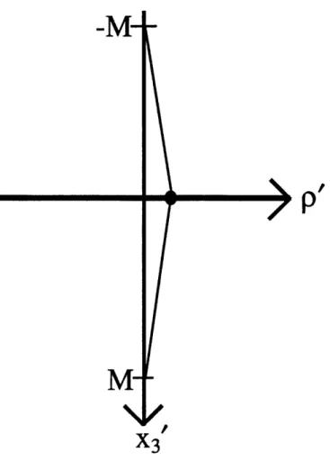
axis, we will not be able to exactly replicate the imaging equations when processing a data set. It is reasonable to assume, therefore, that scatterers located at (pO, x0), such that po is very small (i.e., points very close to the borehole), and x is midway between the first and last source processed, will be best imaged by the algorithm. Since, for these points, the first source may seem to be located at -M and the last source located at M where M is a large number. This is illustrated in Figure 2-2.

(38)

receiver

borehole tool

-source

-borehole casing

--point scatterer

Figure 2-1: A small section of the matrix of cells which make up the imaging region as processed by this algorithm is shown along with the assumed borehole position.

(39)

M-X

3

Figure 2-2: A scatterer located very close to the borehole and mid-way between the first and last source processed will view the source as having moved from -M to +M, with M being a very large num-ber, during the course of the experiment.

(40)

Chapter 3 Imaging Anomalies From

Synthetic Data

3.1 Introduction

We derived in detail a method for imaging anomalies in an otherwise homogeneous medium in Chapter 2. In section 2.3.3 we developed an inversion formula pertinent to data from a 2D medium. The equation thus developed (equation 2.36) is applicable to synthetic data generated on the computer by 2D generating algorithms.

This chapter discusses the results obtained when the algorithm based on equa-tions 2.35 - 2.36 is used to image scatterers from synthetic data for six models. All of the examples in this thesis are from a 2D medium only because codes for generating seismograms from a 2D medium are more readily available and cheaper (in terms of cpu time) than 3D seismograms. By the very acoustic nature of the receivers on the well logging tool, we cannot discern between differing directions around the borehole. Therefore, any real data acquired by such a tool can be considered as coming from a 3D medium made up of infinite, identical vertical 2D slices through a line of sym-metry (namely the borehole). Except for errors in magnitude of the data (some of which we tried to account for in section 2.3.3), the examples should be testimony to

(41)

inversions for 3D data, since we have assumed throughout weak scatterers allowing a single scattering theory to be valid.

We have not taken into account the borehole itself or any fluids contained therein. Meredith (1990) showed that the presence of a borehole and its fluid does not alter the radiation pattern of the Primary (P) wave; there is just a rescaling of the amplitude in the seismograms. The equations in Chapter 2 can be refined to take into account the necessary scaling factors, enabling the algorithm to be applicable to real data from a borehole logging tool.

The six examples chosen to be examined in this thesis represent a few of the anomalies that can be found around a borehole that may be of interest to the explo-ration seismologist.

* Model 1 is a simulation of point scatterers assembled in a somewhat complex

manner.

* Model 2 continues with the idea of point scatterers and assumes that there

are two types of localised scatterers of different velocities (10% and 20% of the background velocity). The aim is to test the algorithm for sensitivity to different magnitudes of localised perturbations. Both models 1 & 2 were com-posed of anomalies that were, in terms of size and velocity perturbations, ideal point scatterers. The algorithm used to generate seismograms from these two mediums was based on Ray-Born scattering, hence multiple scatterings were not present in the data being inverted by the algorithm. It is therefore not surprising that the best results came from these two models.

e Model 3 is composed of a very thin (0.8 of a wavelength) layer, dipping 450

with velocity very close (3%) to that of the background medium, as well as two square regions of differing velocities. These two square regions have sides parallel and perpendicular to the borehole, and it will be of interest to note how the algorithm images these two regions, as they may represent fracture zones

Acoustic modelling of near borehole anolmalies via the generalised radon transform

Acoustic Modelling of Near Borehole Anomalies

via the Generalised Radon Transform

by

Richard Sven Patterson

B.S., University of California, Riverside (1986)

(Physics)

Submitted to the Department of Earth, Atmospheric, and Planetary

Sciences

in partial fulfillment of the requirements for the degree of

Master of Science

at the

MASSACHUSETTS INSTITUTE OF TECHNOLOGY

May 1992

©

Massachusetts Institute of Technology 1992

All rights reserved

Department of Earth, Atmospheric, and Planetary Sciences

C ertified by ...-..

....

. .. .. ...

. . .. .. . .. .

M. Nafi Toks6z

Professor of Geophysics

Thesis Advisor

Thomas H. Jordan

Chairman

Acoustic Modelling of Near Borehole Anomalies via the

Generalised Radon Transform

by

Richard Sven Patterson

Abstract

Acknowledgements

Contents

List of Figures

Chapter 1

Introduction

1.1

Motivation for the Thesis Topic

1.2

Objectives of the Thesis

1.3

Outline of the Thesis

Chapter 2

Theory and Computer

Implementation

2.1

Introduction

2.2

The Forward Problem

2.2.1

Wave Equation in an Acoustic Medium

+

dt

dx

fi

ogg.

dv

dP

d p

(-!)

dO8

+

dt =t

A-V +

M

V

-VP.

|

|

0(E

),

OP

p

of+v

VP=c

0(2),

oi

V

P = 0.

_),

_{P = 0.}

_(2.9)

_x,s)

₊

_{|_}

_{||_}