Granular Ice/Structure Interactions in Flow Conditions

Publisher’s version / Version de l'éditeur:

PERD/CHC Report 5-116, 2004-03

READ THESE TERMS AND CONDITIONS CAREFULLY BEFORE USING THIS WEBSITE.

https://nrc-publications.canada.ca/eng/copyright

Vous avez des questions? Nous pouvons vous aider. Pour communiquer directement avec un auteur, consultez la

première page de la revue dans laquelle son article a été publié afin de trouver ses coordonnées. Si vous n’arrivez pas à les repérer, communiquez avec nous à [email protected].

Questions? Contact the NRC Publications Archive team at

[email protected]. If you wish to email the authors directly, please see the first page of the publication for their contact information.

Archives des publications du CNRC

For the publisher’s version, please access the DOI link below./ Pour consulter la version de l’éditeur, utilisez le lien DOI ci-dessous.

https://doi.org/10.4224/12340985

Access and use of this website and the material on it are subject to the Terms and Conditions set forth at

Granular Ice/Structure Interactions in Flow Conditions

Brown, T.; Tiwari, D.

https://publications-cnrc.canada.ca/fra/droits

L’accès à ce site Web et l’utilisation de son contenu sont assujettis aux conditions présentées dans le site LISEZ CES CONDITIONS ATTENTIVEMENT AVANT D’UTILISER CE SITE WEB.

NRC Publications Record / Notice d'Archives des publications de CNRC: https://nrc-publications.canada.ca/eng/view/object/?id=cc086606-6f41-413c-90f7-69541e48a1ce https://publications-cnrc.canada.ca/fra/voir/objet/?id=cc086606-6f41-413c-90f7-69541e48a1ce

Final Report

On

Granular Ice/Structure Interactions in Flow Conditions

To

National Research Council of Canada PERD Ice/Structure Interaction Program

PERD/CHC Report 5-116

By

T.G. Brown and D. N. Tiwari Department of Civil Engineering

The University of Calgary

I ntroduction

The report addresses one aspect of the issue of granular ice interactions with a fixed structure in a flow regime. The incentive for the work derived from observations obtained from rubble

interactions with the piers of Confederation Bridge. These observations, obtained from interactions with both ridges and rubble fields, indicated that there was little physical contact between the rubble and the pier shaft below the ice-breaking cone, and that there was evidence of significant

disintegration of the rubble feature in the wake of the pier. These suggest that the presence of a significant flow regime (the current can be as high as 1.2 m/sec at Confederation Bridge and 0.7 m/sec is attained on every tide) can influence the failure and subsequent clearing of ice rubble in ridges and rubble fields. As laboratory tests are not normally carried out in the presence of a current flow, it was proposed to carry out a set of such tests.

The report first provides a detailed literature survey of fluid flow past a fixed object and the motion of ice particles adjacent to a fixed object. The report then describes the experimental set-up, model used, and the sets of experiments that were conducted. The report then provides some analysis and discussion of the results.

The tests were conducted in the hydraulic laboratory at the University of Calgary using dye and ice blocks to observe the local currents and the potential interactions with the structure model. The laboratory is not a cold room and so all tests were conducted at room temperature. This provided some challenge in the tests using ice blocks, but there were insufficient observations with sufficient repetition to provide confidence in the qualitative analyses that resulted.

Two video cameras were used throughout the test series and an annotated video of the results is provided with this report.

D

DDooocccuuummmeeennntttMMMaaappp

T

TTeeexxxttt

1 Literature Study 1

1.1 Ice Rubble – Production, Properties, and Interaction 1

1.2 Fluid Flow and Hydrodynamics of Particle Motion 8

1.2.1 Fluid flow about a body in a flume and edge boundary 8

1.2.2 Scale issues 10

1.2.3 Particle movement in a fluid flow 11

1.2.4 Particle movement adjacent to a fixed body 11

1.2.5 Hydrodynamic forces 19

1.3 Inferences from the Literature Study 21

2 Experimental Set Up 25

2.1 Layout 25

2.2 Pier Model 26

2.3 Data Sampling and Acquisition 27

2.4 Experiment Series 29

3 Results and Analysis 31

3.1 Pressure Series 31

3.2 Streamline Series 34

3.3 Ridge Ice Series 39

4 Conclusions and Further Tests/Analyses 43

F

FFiiiggguuurrreeesss

1 Idealized Concepts for the Internal Structure of Ridges and Rubble Field

2

2 Schematic of GPF Model Failure Geometry 6

3 Deviation of Streamlines in Conical Obstruction 10

4 Pressure Distribution around a Uniform Cylinder 12

5 Paths of Particles in flow past a uniform cylinder 13

6 Schematic of geometric relations and forces acting on rotating ice slab 20 7 Tensile stresses around a void in external compression field 23

8 Schematic layout of experiment 25

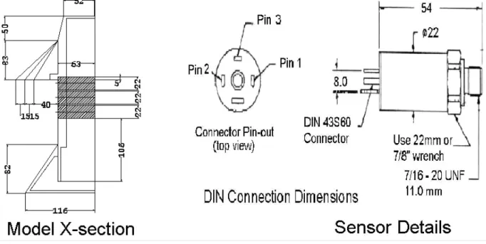
9 Different views on details of the model pier and location of sensors 26

10 Location and details of model and sensors 28

11 Schematic of data sampling points 30

12 Pressure Measurement at high turbulence and high velocity 31 13 Pressures at relatively laminar flow conditions and mild velocity 32 14 Pressures read by the top sensor, flow conditions as in figure (12) 33 15 Experiments with dye revealing the dominant streamlines along

traverse “A” on figure (11)

34 16 Location of zones of increased pressure and velocity due to the

interference of the CONE

35

17(a) Dye particles climbing up the slope of the cone 36

17(b) Dye particles resembling flow around a cylinder at deeper points 37 17(c) Dye particles flowing past underneath the umbrella from the front tip

of the cone

37

17(d) Dye particles in the front zone of the cone 38

18 Traces of pressure sensors during a ridge interaction

19(a) Images during weak ridge interaction 40

19(b) Images during weak ridge interaction 41

19(c) Images during dense ridge interaction

T

TTaaabbbllleeess_s

1 Experimental layout principal measurements 26

2 Model principal measurements 27

1. Literature Study

1.1 Ice Rubble – Production, Properties, and Interactions

An ice sheet deforms when it is acted upon by stresses originating from the interaction with an intercepting structure or another ice sheet. Depending on the sheet thickness and the pack ice pressure, the nature and extent of deformation ranges from crushing and rubbling to rafting and ridging. The rubble build up may also consolidate later to form ridges. So in overall, ridge formation may take place in the far-field and be carried to the structure by environmental forces or it might be formed right in front of the structure; in either case, the interacting ridges are capable of posing the highest level of critical loads to the structure [Croasdale et al, 1995]. Ice ridges with larger lengths, widths, and thicknesses tend to govern the design load, which is the lower of the two extreme cases of limiting driving force and limiting failure stress [Cammaert and Muggeridge [1988]. Hence, the structure and composition as well as the failure mode of the ridges in the special context of an intercepting conical structure merit an in-depth study.

Ice rubble is typically modeled as a Mohr-Coulomb material characterized by a friction angle and cohesion. Friction angle depends on the degree of packing and grain size distribution whereas the cohesion depends on bonding and sintering between the blocks – hence on the

environmental conditions like temperature and salinity etc. Ridges are formed when the broken rubble is held together by friction, buoyancy and gravity forces along with cohesion. Shear ridges, which are formed when adjacent floes move parallel to each other, consist of finely ground ice. Pressure ridges, which are formed when adjacent floes move towards each other, are composed of larger blocks of ice [Parmeter and Coon, 1973]. Since the strength is assumed to be dependent on the size and packing of blocks, it is imperative to look into the production,

consolidation, and failure and disintegration of ice blocks in an ice ridge in the vicinity of a conical structure.

Production and consolidation of rubble

Ice sheet interactions are often accompanied by build-up of rubble on the ice sheet and the cone. Izumiyama, Irani and Timco [1994] have typified the rubble generation process into four categories and suggested that the rubble build up can factor the load up by as much as three times when a sheet of ice (or consolidated layer) fails, predominantly in flexure, against a conical structure. Ice thickness and strength were considered to be the primary influencing factors for the amount and distribution of rubble field, which in turn, influences the load on the structure. It was reported that the smaller rubble particle sizes result in more accumulation in front of the structure and higher loads. Many authors have identified the dependence of rubble size on the parent ice thickness [Sanderson, 1988, Maattanen and Hoikanen, 1990, Mayne and Brown, 2000]. The size of the pieces of ice thus generated can be indexed, if not calculated, by the following equation given by Tatinclaux [1986] –

(01) L = [ _F h/ _w] 0.5

where _F and h are respectively the flexure strength and thickness of the ice sheet and _w is the specific gravity of water.

rubble blocks undergo consolidation at the waterline creating a remolded structure which can again interact with the intercepting structure. The ridge so formed has a distinct sail above the waterline, consolidated (refrozen) layer at the waterline and a keel under the waterline, as shown in the figure (1). The consolidated layer is more solid and competent than the rest of ridge. The keel is weakly fused and all parts of it may not be completely frozen but owing to its depth and extent it is thought to be the major component to contribute towards the load [Sanderson, 1988].

Figure 1 : Source [Croasdale et al, 1996] pp 1-5

Parmeter and Coon[1973] have studied the process of rafting and ridging and proposed an analytical model. They proposed that there exists a certain limiting thickness beyond which ice sheets tend to undergo ridging rather than rafting. Tucker and Govoni [1981] undertook extensive observations in the Prudhoe Bay area and deduced that there exists a strong

correlation between the height of sail, height of keel, area of sail, and the area of the keel to the thickness of the parent sheet. Their empirical equations, in SI units, are as –

(02) h_s = 3.69 √t h_k = 4.57 h_s0.89 A_k = 17.48 A_s0.82

where h_s and h_k are the heights of sail and keel respectively, t is the parent ice thickness and A_s and A_k are the cross-sectional areas of sail and keel respectively.

It is also consistent with the overall hydrostatic equilibrium requirement that the volume of sail should be about 1/10th _{of the volume of keel, so keel depths are about 4-5 times the height of} sail. In first-year ridges, the consolidated layer thickness is about 2 to 2.5 times the parent ice thickness.

Failure of ridge ice and the load on the conical structure

When ridged ice fails against a conical structure, the net load is a combination of the following failure contributions –

• Predominantly flexure failure, possibly accompanied by shear and crushing and, to a lesser extent, buckling, of the consolidated layer followed by clearing (translation, rotation) of the accumulated rubble field.

• Frictional forces encountered in pushing the consolidated layer up the slope (ride-up) in the presence or absence of rubble field.

• Failure of keel against the conical front.

• Sustained pressure exerted by either grounded keel or the trapped blocks resulting from the failure of keel under the water line.

In the failure of consolidated layers, it is acknowledged that for smaller thicknesses, the flexure failure load dominates while for the thicker layers the ride up and clearing forces dominate the highest load. Current models are based on the assumption of the layer being floating completely free in the water while it interacts with the cone. But it should be stressed that there is no clear understanding on how the consolidated layer fails atop the underwater rubble of keel, which might require higher forces to create bending failure, and how it differs from the idealization of a beam on an elastic foundation [Croasdale et al, 1995].

A large ambiguity exists on the understanding of the contribution of the underwater keel part, mainly owing to the momentum likely possessed by its large extent and depth, and the behavior of the rubble as it interacts with the structure. Most of the attempts to explain the failure of keel against the cone and the sustained pressure exerted by the engaged portion of keel in case of a conical front have rather tried to extrapolate and adapt the theories developed for a uniform cylindrical indenter. However, in case of floating keels, the presence of cone and a discontinuous boundary interface at the cone-cylinder junction induces 3-D flow patterns with stagnant and recirculation zones where neither the friction nor the cohesion between the blocks seem to be effectively mobilized to exert any significant lateral pressure to the structure. The same makes

up the major scope of the present study.

Ice rubble is strikingly similar to other coarse granular materials, which have been modeled as Mohr-Coulomb materials. A Mohr-Coulomb material is characterized by a friction angle and cohesion and its strength quantified as –

(03) = c + ’ tanφ

where is the shear strength, c is the cohesion, ’ is the effective normal pressure and φ is the friction angle.

So the same approach gives a good starting point to analyze the ice rubble as well. A failure scenario for a Mohr-Coulomb material comprises of increasingly mobilization of shear strength along a (or many) shear (failure) plane(s) until eventual thorough rupture. In ice rubble, cohesion may be attributed to the freeze bonding between the blocks and the shear friction may be attributed to the packing and distribution of blocks. However, ice rubble departs from Mohr-Coulomb material in three main aspects [Croasdale, 1996]. At the first place, the failure of ice rubble has been reported to be progressive, which implies that cohesion may govern only along an initial portion of the failure plane; unlike other Mohr-Coulomb materials, blocks must be de-bonded before friction can be mobilized. Secondly, at high confining stresses, individual blocks may undergo flexural or local crushing failure at the inter-block contacts. This might be

particularly enhanced at those regions which have been weakened by the continuous weathering of sea-water. Hence, the sizes of blocks produced after failure of rubble/ridge are not necessarily the same as those bonded after sheet-ice has undergone ridging or rubbling. A Mohr-Coulomb material is assumed to have incompressible and infinitely strong grains but ice “grains” are susceptible to breakage and failure, more as in concrete. Thirdly, the internal friction angle and cohesion have been found to be [Urroz-Aquire, 1991 and Sayed et. Al, 1992] dependent upon the normal stress level. Besides, tests of fresh-water ice, which implies that if the φ – c concept did hold proper then it should hold best in the case of freshwater ice manufactured optimistically in controlled labs, revealed that the angle of the failure surfaces and φ along with other rubble behaviors were not reproducible and depended heavily on the loading rate [Azarnejad and Brown, 2001]. Hence the suitability of equation (03) is doubtful.

Typically, most Mohr-Coulomb models of ridge failure calculate either a local passive failure load or a global plug load. A ridge is assumed to fail against a structure in two distinct stages

[Croasdale, 1996]. Initially, the rubble fails downwards generating a passive state of stress, then in the latter stage, a horizontal shear plane forms near the waterline (shear plug failure). The peak load is dependent on both of these stages.

Croasdale et al [1996] have compiled a comprehensive list of failure models of first year ridges and rubble fields. Basically, two approaches have then been improvised. One is the

Dolgopolov/shear plug method which combines the attributes of the Dolgopolov [1975] and shear plug approach and the other is the generalized passive failure (GPF) model, the latter continuously searches for the failure plane giving the minimum load. For model ice ridges and vertical structures, the improved algorithms were validated and the GPF model found to be slightly over-predictive. Several other models analyzing the local or global failure of rubble pile-ups or ridges have been proposed, all of which essentially share the commonality of assuming the ice rubble as a Mohr-Coulomb material [Lemee, 2002], [Nevel, 2001]. Furthermore, most of the models presume the failure planes and uniform mechanical properties which are far from reality.

• Dolgopolov/Shear Plug Method –

(04) 2 0.5 2 (1 )( 2 ) 3 2 e eff p DOl e p h K h P D ch K d γ = + +

where the material is assumed to be Mohr-Coulomb with φ and c being the Mohr-Coulomb friction and cohesion respectively. The coefficient of passive pressure, K_p is given as –

(05) 2

tan (45 )

2 p

K = +φ

The effective buoyant density, γ_eff is given as –

(06) γ_eff = (1-p) (ρ_w - ρ_i) g , p being the porosity

Then, the shear plug model results in an expression for the force on the structure as –

(07)

2

[ tan( ) ] [ tan( ) ] / cos( )

2

plug eff eff i

h

P = γ φ

∫

∫

∫

in which the vertical shear planes are assumed to deviate at an angle ω to the direction of motion.

For the analysis, the actual keel depth at each location, with appropriate surcharge, is used with the Dolgopolov model while an equivalent keel shape is determined for use with the plug model; the algorithm can accommodate triangular, rectangular, trapezoidal, and general three-plane keel bottoms. The minimum of the two loads is then selected as the ridge keel failure load for the structure at that position of the ridge and the position is altered in increments. The peak load is the Dolgopolov or the cross-over load, whichever comes first. The mechanical properties of the rubble as well as the failure plane geometry and the amount of surcharge have to be chosen before the analysis.

• The General Passive Failure (GPF) model –

Figure 2 : Source [Croasdale et al, 1996] pp 3-27

The angle β is the vertical inclination of the primary failure plane. The vertical walls of the failure wedge diverge at angle ω to the direction of ice movement. At a given penetration into the ridge, the model resolves all of the forces acting on the failure wedge to determine the horizontal force for a given β. Thus, at every penetration level, the model hunts for a critical β corresponding to the minimum load. The model is capable of taking into account non-vertical structure, wall friction, inertia and buildup of surcharge in front of the pier during penetration.

Croasdale et al [1996] also did a few series of model tests on conical structures for verification purposes. The penetration speed showed little effect on the load. It was also reported that a fair correlation exists between the depths of the keel to the net horizontal load experienced by the structure.

In order to get real-time full-scale data on failure of ice, two of the piers of the Confederation Bridge have been calibrated and instrumented, the traces of which are being continuously logged [Brown, 1997]. This real-time data, however, reveals some very contrasting results. Lemee [2002] did a regression analysis of 71 keel interaction events for relationship between keel depth and load and found that there exists no such relationship. By analysis of the data from the pressure panels embedded in the zones above and below the cone in the piers, he has also reported that there is no relevance of wetted depth of the cone to the net load nor is there any sustained pressure by the broken ice rubble as such under the cone. He admits, though, that the level of

load peaks in relation to the penetration of the thickest part of the ridge and drops down again during a single event. As supporting evidence, Lemee [2002] has pointed out the underwater video depicting sea life existing for more than a year, which should have been brushed off and impossible to have been grown, if the rubble did behave according to the existing theories. On the other hand, regarding the behavior of grounded rubble, Timco [1993] did a model study on the load transmissivity of grounded rubble. He noted that the frictional resistance gradually increased contrary to the assumption of fully-mobilized frictional resistance. Furthermore, he reports that the ratio of the lateral force transmitted to the structure to the total horizontal force decreased with the decreasing ratio of vertical force on the structure (berm of the Molikpaq structure) to the total horizontal force.

From these discussions and especially noting the following points –

• large disparity of model predictions to the real-time full-scale observations from the Confederation Bridge in the magnitude of load on a single event as well as comparability between two events identical in terms of Mohr-Coulomb approach

• lack of evidence supporting the dependence of peak loads to the keel depth and lack of a single evidence of existence of sustained pressure by the broken rubble

• departure of the ice rubble behavior from ideal Mohr-Coulomb nature in terms of non-concurrent mobilization of cohesion with internal friction, gradual build up and

mobilization of internal friction, dependence of internal friction on the normal stress level and rate of loading, and likelihood of trans-block crushing and bending failures as well as high stochastic nature of failure planes

• behavior of grounded rubble departing from that as predicted by a Mohr-Coulomb material

It can be deduced that the Mohr-Coulomb approach may not be the proper approach to explain the failure of keels and failure of ridge ice, at large. Furthermore, Lemee [2002] cites the work of Bruneau (1996) who obtained strength equations from a regression analysis of almost all the available test data –

(08) φ = 1.22 – 168b_t + 1.37 p c = 1624 b_t – 7

where b_t is the block thickness and p is the porosity.

Contrary to the popular belief that denser materials should produce higher friction, it shows that porosity increases the friction angle. Mainly because similar ridges (comparable keel depths and widths) failing under similar environmental conditions attribute appreciably varying peak loads, and the peak load itself is dependent on the geometry of interaction, the role of porosity, in particular, is further stressed. Confusion as to whether the continuous or peak shear have been reported could have been one factor but the fact that it comes from a regression analysis and that porosity influences the strength to such a large extent suggests that the Mohr-Coulomb approach might not be the best one.

However, in case of grounded rubble, it is likely to act as a Mohr-Coulomb material as the effect of water as a disengaging and suspending medium will be less prominent, and the friction will still be likely to be mobilized through the inter-block contact interfaces.

1.2 Fluid Flow and Hydrodynamics of Motion of Particles

The motion of a particle suspended in a fluid medium depends primarily on the flow regime and the shape and density of the particle. Moreover, if there is a bunch of particles, their motion is also governed by the nature and extent of the interaction between them. In the typical case of flow of ice rubble along a water stream, it is obvious that the pattern of flow is very complex. Several techniques exist that permit the modeling of such a phenomenon. Computational Fluid Dynamics (CFD) techniques based on finite element methods are being used with a fair degree of success. The methods involve first solving a general differential equation of motion of fluid dynamics in a region within known boundary conditions, for example the Navier-Stokes equation, which would give the velocity field in the boundary region of flow stream.

Consequently, the static ( = ρgH, H being the height of fluid column) and dynamic ( = 0.5 ρ V2, V being the velocity) fluid pressure are calculated, an integration of which over the particle submerged surface gives the force on the particle and hence its motion. In the case of the interaction of a chaos of particles of varied shapes and sizes, the topology of the particles should be known as the input and the same can be modeled as a system of “links” that is solved with appropriate mathematical models, say – dynamics of tree structures. The interactions between the particles can also be incorporated in such models. These models have been successfully used to model the discrete particle flow mechanics in different flow patterns, for instance, debris flow, ice jams etc. [Gresho and Sani, 2002], [Pironneau, 1989].

However, in the case of the interaction between drifting ice and a stationary structure, the main problem that arises is that neither the topology of the particles is exactly known nor is the

interaction between them. Unlike river jams where ice is predominantly flaky and originates from an identifiable crystal size to an identifiable frazil size, particles of every shape and size

imaginable can be produced in an ice-structure interaction. So these methods, at their best can only give an approximation to the actual behavior. Next, these methods are very much sensitive to the boundary conditions and thus the solution of a particular problem holds well only for that problem and deductions of generalized inferences are not generally supported. And the presence of 3D flow patterns, waves and turbulence in real offshore environments further complicates the solution.

Given the popularity for conical front structures in ice-infested waters and the complexity of the ice-structure interaction, it is imperative to examine the various facets of the production, traits, and trajectories of interacting ice particles by experimental means. However, the disparity of the flow regime between the experimental set-up and an actual offshore environment should be well understood before the experimental results are applied to the full-scale structure.

1.2.1 Fluid flow about a body in a flume and edge boundary

Several equations exist, empirical and semi-empirical, that model the gravity flow of fluid in a flume. Manning’s equation is a popular method but demands appreciable wisdom in the selection of the roughness coefficient. Similarly, other equations like the Chezy’s equation, also possess the same merit. The following derivation provides an equation that best describes qualitative

analysis of the flow and its regime and its differences with an offshore flow condition [Milne-Thompson, 1981].

If v is the constant velocity parallel to the walls and h is the depth of gravity flow in a rectangular channel with a flat bed of width b, application of Bernoulli’s equation at the surface gives; v2 + 2gh = constant

If the breadth of the channel varies slightly, there will be a small consequent change in v, and therefore by differentiation,

(09) v dv + g dh = 0

Again, from the continuity equation, vbh = constant, which gives,

(10) dv/v + db/b + dh/h = 0

Eliminating dv between (09) and (10) gives the following relation –

(11) 2 2 ( ) dh v h db =b gh v−

But c2 = gh where c is the speed of long waves in open water.

This reveals that the depth and breadth increase together, if and only if, v < c. Therefore, a free gravity flow for a given bed material and slope associates a unique combination of flow depth and velocity and to control one of them while keeping the other fixed requires the introduction of a control mechanism such as a gate. Furthermore, as a thumb-rule, the effect of boundary layer at the edges will be prevalent up to 1/3rd of the total width in a narrow rectangular channel. So, the middle third can be considered relatively free of edge boundary effects.

On the other hand, the flow around a conical structure is very complex, primarily because it is three-dimensional. Considering a potential flow on a plane parallel to the flow, the middle streamlines, which strike the cone before the edge ones do, tend to deviate, still parallel to the flow surface, around the periphery of the cone in a 2D- fashion similar to that of a flow around a uniform cylinder. However, there is a mismatch of the flow between the immediate upper and lower of such planes. This has an effect that the streamlines on the edges first glide up and traverse along the cone surface, in the plane of the elevation of the cone, then deviate radially outwards and eventually merge in the wake further downstream, as shown in figure (3).

Figure 3

Viscous flow in such a configuration is accompanied by eddies and recirculation zones in the front and side directions plus vortices in the wake. In the particular case of a cone being joined to the cylinder and the junction lying in the submerged region, there is a flow disruption at the interface that induces eddies and reverse flows with stagnant zones formed in the portion under the projected umbrella and down to a depth varying around the circumference and depending upon the flow velocity and the projection of the conical umbrella from the cylinder. Thus, besides the obvious governing parameters like the flow velocity V, Reynolds number R, Froude number F etc, the flow in such a case is also dependent upon the geometric parameters of the structure. It is then intuitive to attempt to investigate the flow pattern itself in terms of the variables d and D, besides the regular flow parameters, where d is the diameter of the cylinder and D is the diameter of the cone, as in figure (3).

1.2.2 Scale issues

Inertial, gravitational and viscous forces govern the forces that drive the motion of an object through an incompressible fluid. Froude number is the ratio of inertial to gravitational forces and Reynolds number is the ratio of inertial to viscous forces. In this case, equality of Reynolds and Froude number between the model and prototype ensure exact modeling, however, the

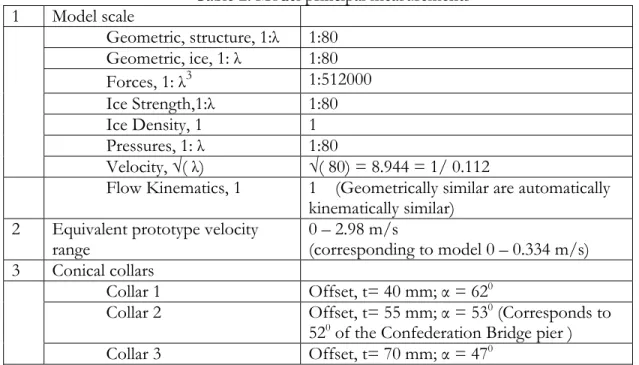
simultaneous equality of both the model and prototype Froude and Reynolds numbers is impossible if the same fluid medium is used [Street et al, 1996]. The usual technique, then, is to equalize one of the numbers and correct the so obtained results for the other number. Where surface waves are deemed to be the predominant excitation mechanism, Froude scaling is adopted [Lever et al, 1983]. As a pre-calculation, as the geometrically similar flows are automatically kinematically similar, then the dynamic similitude considering Froude similarity would require:

(12) ( )mod ( )

lg_n lg_n ptp

V ₌ V

It follows that for a scale of 1: λ = 1: 80, the model velocity should be 0.112 times the prototype velocity, maintaining which would serve no good for the study of ice breaking in ice-structure

interactions. However, such a scaling in velocity would serve good enough for the trajectory of the particles as both the buoyant and drag forces will scale in the proportion λ3.

Scale issues also depend on the size of the particle itself. It is well-known that, based on the size of the particle relative to the flow regime, if the size is too small, the particle behaves as a fluid particle, in which case particle flows due to fluid pressure. At intermediate sizes, the viscous forces tend to dominate, while if large enough to cause interference to the flow regime around it, the gravitational forces tend to dominate [Lever et al, 1983]. This relation has been elaborated on in the respective sections that follow.

1.2.3 Particle movement in a fluid flow

As previously stated, the flow of a particle in a moving fluid depends on the density, size and shape of the particle. Given that the particles will be at least suspended in stationary water in terms of their density, viscous forces tend to govern for relatively small sizes and gravity forces are significant when the size is large enough to cause interference with the flow. From

experiments with models of icebergs and bergy bits in flow conditions also involving surface waves, it has been reported in [Lever et al, 1983] that the wave-induced ice motion has its upper and lower limits, where viscous forces are negligible, definable in terms of the ratio of the particle size to the wave-length. In the case of particles with the ratio less than 0.077 (=1/13), the particles behave as fluid particles and their motion is essentially due to the pressure field associated with fluid accelerations (Froude-Krylov force). The relative motion between ice and fluid will be small resulting in small viscous forces. At ratios between 0.077 and 0.1, shape has an identifiable effect on the trajectory of the particle. At ratios larger than 0.077, wave diffraction and generation effects due to the body’s own motion are significant enough to affect the motion of the body.

1.2.4 Particle movement adjacent to fixed body

The interference caused by a fixed body has the effect of changing the pressure and velocity fields in the flow medium around it. A typical ice-structure interaction involves production of particles of every shape and size at the interacting front. For sake of simplicity, the particles can be supposed to have been “introduced” inside or vicinal to the zone of interference of flow by the structure. Smaller particles glide along the space velocity vector while larger particles interfere with the flow. For the particle in the vicinity of the recirculation zone, it has a net effect of outward deviation, the magnitude of which depends on the size of the particle. For the particle already within the recirculation zone, the net effect is that the speed is slowed down, sometimes even reversed [Vinogradov and Croasdale, 1987], and the path elongated – which again implies that the particle is repulsed from hitting the structure.

The solution for a typical case of interception of flow by a uniform cylinder in inviscid flow reveals that pressure changes significantly around it. Setting aside the eddy effects in the flow itself, as viscous forces have very little effect on small particles, the “ideal” solution holds well for “real” cases.

The hydrodynamic pressure, p, at a point of the cylinder intercepting an inviscid and incompressible fluid flow is given as –

(13) p – Π = ½ ρU 2 (1 – 4Sin 2 )

where Π and U are respectively the total pressure and speed at infinity (the speed at the normal points A and B is 2U ).

Figure 4 : Pressure Distribution around a Uniform Cylinder, Source [Milne-Thompson, 1981] pp 161

Taking the radius a to represent the pressure Π, and plotting the distribution in a polar diagram as in figure (4), we see that at points N1, N2, N3 and N4 at angles 30

0_{, 150}0_{, 270}0_{, and 330}0_{, the} pressure is Π. Along the arcs N4 LN1 and N3 MN2, the pressure exceeds Π , the excess being ½ ρU 2

while along the arcs N1 AN2 and N3 BN4, the pressure is less than Π, the maximum defect being (3/2)ρU 2

.

The solution for the trajectory of a particle approaching a cylinder shows that the particle takes up an orbital path and flows past after a series of orbits.

The radius of curvature R of a particle when the fluid is streaming past the cylinder is given as –

(14) 1/R = (4/a2) (y – ½ )

where is the streamline of the particle at Cartesian co-ordinate y with the center of the cylinder as the origin.

The drift of particle can be evaluated and expressed as elliptic integrals assuming the motion of cylinder in a stationary medium, which is hydrodynamically equivalent to streaming fluid past a cylinder [Milne-Thompson, 1981]. Such a path can then be plotted as shown in the figure (5).

Figure 5 : Paths of Particles in flow past a uniform cylinder, Source [Milne-Thompson, 1981] pp 243 & 245

With the origin of time as the moment of central passage of the cylinder, the numbers on the curve record the times at those points in a suitable unit. For instance, the number 2 means the position of the particle when the cylinder has moved 2 radii from the centre position. The dashed curved line on the left shows the initial positions when the cylinder is at -∞ and the dashed line on the right show the final positions when the cylinder has passed +∞.

However, when the size of the particle becomes more significant and the geometry of the structure less like that of a uniform cylinder, as it does in reality, a closed form solution for the particle also becomes less of a possibility. When the medium is viscous and surface waves are present, the solution becomes more complexity. Many attempts resorting to computational solutions have indeed been made but their shortcomings lie in the extent to which they represent reality. The following sections include some prominent cases of such attempts.

• Motion of particles around a fixed body: Isaacson’s numerical solutions

Isaacson [1987], [1988] carried out a very comprehensive analysis for the numerical solution of the motions of approaching ice masses near a structure in an offshore environment, taking into account the simultaneous hydrodynamic effects of the waves as well as the currents. His main argument has remained to be the profound effect of wave-drift forces and hence the possibility of typification of flow patterns via Froude numbering.

In [Isaacson, 1987], the ice mass is assumed to have two types of motions- (1) wave-induced oscillatory motion, which is treated by application of linear diffraction theory and (2) drift motion treated by a time-stepping procedure applied to drift equations of motion, which involve zero frequency (zero Froude number) added mass, drag forces, and wave drift forces. While considering the effects of interaction of waves and currents in the presence of ice mass and structure – the calculation of oscillatory motion of the ice mass at any particular

location along the trajectory is based on the quasi-steady assumption that the ice mass has a fixed equilibrium position at that instant, which is justified as the time scales of oscillatory and drift motions are generally very different.

Three distinct flow regimes are outlined based on D_i/L – the ratio of size of ice mass, D_i to the wave-length, L. For D_i/L < 0.2, wave diffraction from the ice mass becomes negligible and the ice mass behaves essentially as a fluid particle following the orbital motion of the fluid itself although oscillatory motions may be increased by resonance in heave, pitch and roll. For 0.2 < D_i/L < 2, the wave diffraction and radiation by the ice mass and also the wave diffraction by the structure are significant. For D_i/L > 2, oscillatory motions of the ice mass become negligible.

o Oscillatory motions –

To solve for the oscillatory motions of the ice mass, the flow is taken to be irrotational so that it may be described by a velocity potential φ that satisfies the Laplace equation within the fluid region. The ice mass oscillates with six degrees of freedom corresponding to surge, sway, heave, roll, pitch and yaw. Each mode of motion is harmonic and can be expressed in the form _k exp(–i t) where t is time and _k is the complex amplitude of each component motion. The flow potential is made up of components associated with the forces due to each of the six oscillatory motions, incident wave and scattered waves, the latter two being

proportional to the incident wave height.

(15)

}

∑

where H is the incident wave-height, (k = 1 to 6) corresponds to the six oscillatory motions, φ₀ is the known incident wave potential and φ₇ is the scattered wave potential. The unknown flow potentials, φ₁ to φ_7, which are generally complex, are solved by a discretization procedure as –

(16) ( ) 1 ( ) ( , ) 1,....7 4 k k S x f G x dS k φ ζ ζ π =

_∫

where f_k( ) is a source strength distribution function, is a point on the surface S – the submerged equilibrium ice mass surface over which the integration is performed, and G(x, ) is a known Green’s function for the general point x due to a source of unit strength located at .

Once the source strengths have been evaluated, flow potential is known, an integration of which gives the wave drift force and other hydrodynamic parameters. Then the wave-induced excitation force F_j’, added mass µ_ij, and the radiation damping coefficient λ_ij are given as –

(17) F_j’= –ρ 2 ∫_Si (φ₀ + φ₇) n_j dS µ_ij= –ρ Re{ ∫_Si φ_k n_j dS} λij= –ρ Im{ ∫Si φk nj dS}

where n_j is the unit outward normal to the submerged equilibrium surface S_i of the ice mass.

The equations of motion for the oscillatory motions of the ice mass then may be written as – (18) ( ) ' ' 6 1 2 ] ) ( ) ( [ jk k j v jk jk jk jk k F c i m + − + + = −

∑

where m_jk are the mass matrix components, c_jk are the hydrostatic stiffness matrix components, λjk(v) are empirical viscous damping coefficients, and k

’

= 2 k/H are response amplitude operators that are obtained from these equations.

The response amplitude operators describe the ice mass responses for the incident waves. o Drift Motions –

The ice mass has three degrees of freedom corresponding to drift in surge, sway and yaw. For simplicity, yaw is ignored. When the ice mass diameter to the structure diameter ratio D_i/D_s is sufficiently small, the ice mass is considered to be located in the non-uniform current field produced by the structure, otherwise the current field is uniform. So depending on D_i/D_s, the trajectory is calculated on a uniform current field for large ratios and on a non-uniform field for small ratios. The velocity potential φ is composed of incident current flow φ_c, and the linearly added disturbance potential φ_d in case of non-uniform current field. φ_c is known a priori and following the same logic as before, φ_d is calculated by representation as due to a distribution of point sources around the submerged structure surface as in

equation (16), a differentiation of which yields the velocity components in the directions of the degrees of freedom (dof).

The forces acting are mainly the wave drift and the current drag forces. The wave drift force F_i(w) is obtained from the diffraction calculation as before. The drag force F_i(d) is given as

(19) F_i(d) = ½ ρ A C_d u_i(r) |u(r)| i = 1, 2

where u_i(r) is the current velocity vector relative to the ice mass in the ith dof, C_d is the drag coefficient and A is the projected submerged area of the ice mass onto the plane perpendicular to u(r)

.

Then the equations of motion can be written and solved by time-stepping procedures as –

(20) (m + µ_i) = F_i(d) + F_i(w) i = 1,2

where µ₁ and µ₂ are the added mass components in the respective dofs. The co-ordinate system is moving as quasi-steady equilibrium is assumed to hold at each instant.

The system of equations was numerically solved and the effect of wave drift force on the trajectory studied [Isaacson, 1988]. It was deduced that the wave drift force is important in establishing the ice mass trajectory as it counteracts the current drag at zero drift acceleration and the ice mass travels faster than the ambient current. Similarly, the drift trajectory might be asymmetric owing to the influence of the drift forces acting at an angle to the current direction. The proximity of the ice mass to the structure (usually in the range of 0.1 times the diameter of the structure) manifests the interference of the structure to the local motion of the ice mass.

In a later study for the influence of wave drift force on ice mass motions, Isaacson [1988] contends that as the ice mass size increases, the wave drift forces are actually more important than any other force in the determination of trajectory of the ice mass near a structure in an offshore environment.

The wave drift forces may be calculated by rigorous solution of the wave diffraction theory as in the earlier section. However, as a simple aggregation, the wave drift force F_W may also be conveniently expressed as,

(21) F_W = ½ ρ g C_WDH2

where C_W is the coefficient of wave drift force, D is a characteristic horizontal dimension and H is the wave height.

For a free floating ice mass in a steady, uniform current, the velocity after time t is given as,

(22) U(t) = U_C ( 1 – 1 / [ 1 + U_C t /D ] where U_C is the free stream velocity.

In calm waters, the velocity of ice mass gradually attains the free stream velocity but the presence of waves has the effect of raising the asymptotic equilibrium velocity. Similarly, the presence of a structure distorts the current field so that the drift force depends on the relative position from the structure. It has been seen that the coefficient of wave drift force, C_W varies cyclically with distance from the structure. From dimensional analysis and

experiments, C_W is evaluated for a combination of parameters as:

(23) C_W = f ( D/L , h/D, h/d )

where L is the wave length, h is the ice mass draft, and d is the water depth. Drag forces may be evaluated as –

(24) F_d = ½ ρ h C_D D U_r 2

where C_D is the coefficient of drag and U_r the relative velocity between the ice mass and the dragging medium like current, wind etc.

Then a representative drift equation of motion can be written as:

(25) = A cos(kx) + B (U_C – U) |U_C – U|

where A and B are the parameters describing the relative magnitude of the wave drift and drag forces respectively, and k is the wave number.

Solution of this equation gives U and it has been found for sufficiently large values of A/B that U might be negative. It reveals that if the wave drift forces are sufficiently large then negative drift of the ice mass will occur.

Hence, it has been pointed out that the wave drift forces play a significant role in

determining the trajectory of the ice mass and in some cases lead to rather sharp changes in the trajectory as deviation away from the structure as well as even negative drift of the ice mass.

Nevertheless, the flow of broken ice pieces does not always involve a single piece, in fact many pieces are involved which interact not only with the hydraulics of the regime but also with themselves. An investigation, then, into aggregating the flow characteristics in more familiar parameters, if successful, would be highly desirable. An experimental examination on frazil flocs and particles shows some interesting results as follows.

• Experiments on frazil flocs by Park and Gerard

Park and Gerard [1984] experimentally investigated the formation of freeze-up in rivers for the hydraulic characteristics of disc-like frazil flocs as they form throughout the flow, flocculate, and when turbulence is not too high, gradually rise to the surface to eventually form frazil pans. The rise velocity of the flocs is identified as a key parameter and its dependence upon several hydraulic parameters was one of the desired outcomes. Rise velocity itself is dependent on the drag coefficient. The drag coefficient was found to be dependent on Corey’s, or ‘flatness’ shape factor {= L_min/ √( L_max × L_med) where L_max, L_med, L_min are the three orthogonal dimensions of the floc} but unaffected by the floc porosity and floc bulk density. The drag coefficient was found to be significantly larger than that for an equivalent sphere which is attributed to the surface roughness although there existed little dependence to the floc Reynolds number, which is also a measure of the surface roughness. The problem of disc-like particles in the flow interference of a structure including mutual interaction has been also modeled numerically. The following vessel-interaction and ice jam model is one such but involves only the interactions on the free water surface.

• Vinogradov’s vessel-interaction and ice jam models

Vinogradov [1986] has presented a simulation model of vessel-ice floes interaction in the plane of the water surface. To take into account the variability of the floe geometry and mutual interaction, three different level objects are designated – the floe being the simplest one characterized by random geometry of the contour and mass, a cluster of floes being the intermediate one characterized by number of floes and the contact coordinates, and the combination of isolated floes and clusters being the highest one. The act of ship-ice collision constitutes an event which results in either a ship-floe system or ship remaining as an isolated object. A next collision may result in a two floes-ship system or one floe-ship system and an isolated ship system and so on. The motion of ship with attached object and motion of floes are assumed to be independent in the time interval ∆t.

The ship is assumed to have six degrees of freedom. The floe objects are modeled as “trees” which also have six degrees of freedom. The separated equations of motion are solved – the ship system and the tree dynamics of floes for each time interval, and new states are updated. Altogether, this presents a viable methodology to bring into account the effects of the

interaction of ice particles as a system per se as well as with an external system of structure or ship.

A separate model by Vinogradov [1992] deals with the motion of broken ice in simulation of situations such as river ice jamming. The model is also based on a discrete system approach

and involves time-stepping solution of equations of motion of “tree” structures. The

topology (location vectors) of each floe was described by a tree which was used to generate a set of simultaneous algebraic and differential equations of motion. It has been identified that the amount of coupling between the regime of water flow and ice motion may vary

depending on the densities of the ice floes on the water surface. Also the trajectory of the ice particles depends primarily on the drag and lift forces which are dependent on the topology and geometry of the particles themselves and the relative water velocity, which can be solved for in this model.

The following numerical model solves the problem of an ice mass approaching a cylindrical structure, but without accounting for diffraction and interference effects due to the cylinder and the ice mass itself. The flow is assumed to be laminar and the translational and rotational

motions of the ice mass along the deviating streamlines in 2D are formulated. • Vinogradov-Croasdale ice mass - cylinder model

Vinogradov and Croasdale [1987] acknowledged that the magnitude of impact force a drifting ice floe can exert on a stationary structure and even the clearance of the ice-rubble around a structure can be affected to a great extent by the hydrodynamic forces prevalent at the interaction face. In some combination of flow parameters and the geometry of the ice floe, the floe can deviate sufficiently far from the structure thereby avoiding any kind of collision.

A model is presented to solve numerically the kinematics of a discrete ice mass for

hydrodynamic effects. The trajectory of the floe is a balance between the inertial, drag, and viscous forces in the potential flow field affected by the structure, the vertical cylinder. A floe experiences the drag resistance due to the deviation of its trajectory from the flow streamline, the rate of the deviation (the relative velocity) being proportional to the magnitude of inertial forces. However, the mass also corresponds to a smaller rate of angular acceleration.

The floe is assumed to be comprised of a number of disks. The overall drag force and moment can be computed by integrating the dynamic pressure over the surface S,

characterizing a plane coordinate on the projected area normal to the direction of motion, and the equations of motion can be written in the form –

(26)

∑

( && & &

(27)

∑

( ψ&& & &

subjected to the initial conditions at t = 0; U₀ = U_∞; | ₀| = V_~ ; = 0 ; = 0 q_j = 0.5 ρ C_Dj A.

where m, I are the floe mass and moment of inertia respectively, m_a, I_a are the added mass and added inertia, U₀ is the position vector of the center of mass of the floe from the center of the cylinder, is the angle of rotation about the center of the mass, V_j is the streamline velocity vector associated with the center of the jth disk, U_j

is the velocity vector of the jth disk, R_jo is the position vector of the center of the jth disk in the local system of coordinates; V_~ is the velocity of the current or wind far away from the structure, C_Dj is the drag coefficient of the jth disk and A is the area of the jth disk.

For the case of a cylinder, the velocity of streamline is given as,

(28) V_j = ( 1- R2/U_j2)

And the velocity _j as,

(29) _j = ₀ + × R_jo.

where R is the radius of the cylinder, U₀ is the velocity vector of the center of mass in the global system of coordinates, and is the vector of angular velocity. Time-stepping solution of the above equation of motion yields the trajectory of the ice mass.

Solutions for different sized masses were obtained. It was observed that the rotation of the floe increases with the increase in the mass. Also, the larger the mass, the straighter the trajectory it traverses. It can be summarized that the hydrodynamic forces can significantly affect the trajectory but the effects being more profound for smaller ice masses. This approach, although 2D, also seems to be applicable to model the clearing of ice in the interaction front.

1.2.5 Hydrodynamic forces

Frederking [1979] has given expressions for the hydrodynamic force on an ice block interacting with the structure.

The hydrodynamic force F_h on a rotating slab at a sloping interaction front is given by –

(30) 2 ( ) 2 2 d b h w C l F = ρ A φ& φ = – Sin–1 _{{Sin (1- V t / l} b )

where C_d is the coefficient of drag, A is the cross-sectional area swept by the rotating ice slab, V is the rotational velocity, t is the time increment unit, and is the rotational velocity of the block of length l_b .

Figure 6 : Schematic of geometric relations and forces acting on rotating ice slab, Source [Frederking, 1979]

1.3 Inferences From the Literature Study

A study of the literature reveals that because of its striking similarity to geotechnical materials such as coarse granular materials, several efforts have been made to apply geotechnical principles in the case of ice ridges. Furthermore, the effect of water-borne hydrodynamic forces has been rarely taken into account in such models. This presents with a vague option of whether to treat the ridge as a rigid body or a conglomerated φ – c material. Regarding the φ – c notion, there exist some significant discrepancies between the two materials. Especially in case of conical structures, the departure of ice rubble from a typical Mohr-Coulomb grain distribution and the disparity of the “load” theories become clearly evident. Real-time monitoring of the

Confederation Bridge has also provided sufficient evidence to undeify the φ – c approach. Progressive nature of failure, viz., de-cohesion followed by “shear mobilization”, trans-granular breakage, and dependence of cohesion and internal friction angle upon normal stress and loading rate as well as an inverse dependence on porosity imply that the following suggestion deserves due attention –

• The portion of the keel that remains submerged may not be behaving as a Mohr-Coulomb coarse granular material but rather the individual particles become suspended in the water and randomly detached from each-other (or randomly connected but incapable of transmitting a net load in the direction lateral to the structure), especially due to the buoyancy effects, which clears away from the structure as soon as it gets a favorable current of least resistance. This essentially means that, at least in the special context of a conical structure collared to a cylindrical base structure as in the

Confederation Bridge piers, the submerged portion of the ridge mass lacks enough frontal contact to exert a sustained pressure and once broken, the particles become disengaged and suspended in water, with a net effect of mobilized friction equal to naught, analogous to a quicksand condition. Instead, the mechanics of interaction between the particles will be more like that of mutually impacting particles in a debris flow.

Regarding the kinematics of ice particles under different flow conditions, varying views have been proposed. Especially in the case of an offshore environment, the effects of wave-drift forces, hence the free-stream velocities have been identified [Isaacson, 1987, 1988], [Lever et al, 1983]. Experimental as well as numerical studies have been conducted to support the same. Furthermore, several models have been proposed to model the kinematics of ice particles in different kinds of idealized flow conditions. However, most of the models deal with kinematics of a single block of ice. Even the models taking into account a system of particles make such simplifying assumptions that barely represent reality. However, there is a general agreement that there exists a threshold particle size (the diameter or a characteristic shape index) determined by the flow regime and the density of the particle, below which the particle behaves essentially as a fluid particle and above which there is a coupling effect as the particle itself interferes with the flow.

Another factor affecting the flow regime is the interference of the structure. Three-dimensional flow always exists around a conical structure. In the case when the cone just “hangs” collared to a cylinder, the flow pattern is even more complex as shown in figure (3). There is an obvious dependence of flow regime on the geometrical parameters like the wetted depth of the cone and

the diameters of the cone and the cylinder. Moreover, the kinematics of the flowing particle also depends on these geometric parameters. Where the wave-drift and buoyant forces dominate, the kinematics depend on the diameter of the cone/cylinder (D), diameter of the particle (d), draft of the particle (h), and the height of the wave (H) besides the flow velocity (U_r) [drift force D, H2 and current drag D, h, U_r2 and U_r generally R2/V2_flow for a cylindrical interference, R being the radius of the cylinder]. In case of rotational motion and the behavior of a system of particles, the distance of the (system of) particle’s center of gravity (cg.) from the interfering structure also governs to some extent as this decides the level of interference caused by the structure and the deviation likely to be taken up by the (system of) particles. In case of flaky particles, the shape index and Reynolds number influence the velocity.

Based on these discussions, it can be concluded that the motion of particles is affected by so many parameters that an experimental investigation for the kinematics against each particular variable would be quite revealing but only in terms of some limited qualitative aspects. Although, all such hydrodynamic effects can be aggregated as agents of change in angular momentum, as in equation (30), a representative measurement of the rotational velocity will again be a matter of crude and uncertain approximation. Therefore, for sake of amenity and comprehensibility, efforts to investigate experimentally, obviously accompanied by analytical studies, the kinematic behavior should be more directed at identifying non-dimensional homogeneous groups such as Froude number, Reynolds number, shape index, d/D etc and study the relationships in terms of the same.

The dependence of the peak load to the loading conditions and geometric configurations, the variation of peak load even under otherwise “identical” loading conditions and irrelevance of keel depth to the magnitude of the net load experienced, plus the strong dependence of peak load on the porosity, suggest that a fracture mechanics approach may be more appealing than a Mohr-Coulomb local or global failure scheme.

The role of cracks have traditionally been accounted for by taking a reduced effective section (area, moment of inertia etc) but the development of fracture mechanics has now led to successful explanation of various failure mechanisms on the basis of propagation of the crack itself.

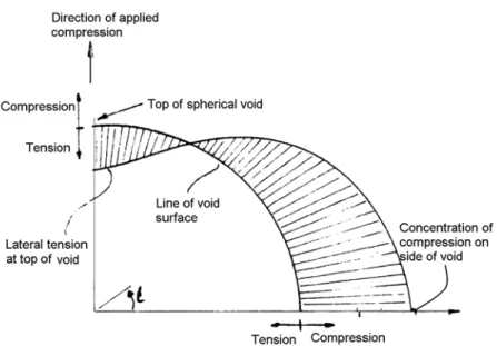
Figure 7 : Tensile stresses around a void in external compression field

Looking from a different perspective, of stress around a void as shown in the figure (7), it can be seen that the porosity of the ice- hence the size of the pre-existing flaw, governs the load exerted on the structure. As the compressive stress “flows” around a void, regions of tensile stresses are produced in the lateral direction which might be sufficient to propagate the pre-existing flaw (of the size of the diameter of the void). When sufficient cracks

coalesce, a final failure would occur. Furthermore, it is not always observed that the ice body fails along the direction of the indenter (like an axe through wood, by the way the edge of the cone also lacks enough frontal contact area) as is evident from the observation of “plug” failures. However, ice can fail along or normal to or at any direction to the direction of indenter. This also supports the dependence of the failure of ridge-keels on the shape and size of pores.

A proper recognition of the range of porosity can give a better insight into the range of the size of pre-existing flaws, which in turn, govern the total load experienced by the structure. If the ridge is homogeneous enough, then this type of model would predict that the load will rise until the first breakage of the ridge, in tandem with the level of penetration, and then reduce. The uncertainty in the duration of interaction events can also be explained by the fracture mechanics approach as the continuation and seizure of propagation of cracks will be governed largely by the environmental driving forces and the loading configuration encountered at the interacting front. No matter whether the ridge thus first fails locally or globally, the smallest flaw in the largest piece so formed afterwards will again most likely govern the next peak in the load history. This also explains the stochastic variations in the loading history of the ridge-ice interaction events. Furthermore, non-simultaneous failures will also induce more randomness into the process. So on and so forth, when the piece size reaches a situation when it can be swept or cleared away from the structure, then it surely will. Such a size will be decided by the flow regime (flow conditions and structure geometry) and the confinement provided by the ice-cover. Smaller particles will act more like fluid particles whilst larger particles will interfere with the flow regime as well.

This implies that the existing Mohr-Coulomb passive pressure or shear failure theories or plug theories need reconsideration, at least in the special case of conical structure like the piers of the Confederation Bridge.

2. Experimental Setup

The experiments are set up in the hydraulics facilities of the Department of Civil Engineering at the University of Calgary. A regulated discharge is passed through a gate-controlled flume in which the instrumented model of the Confederation Bridge pier is mounted. Tests were

conducted for three different series. In one series, the change in pressure field around the piers, as an effect of the conical collar, was determined. The next series consisted of introduction of color dyes and small ice pieces to track the significant currents and streamlines of the flow around the pier. Subsequently, ridges of ice rubble were pushed against the model. The flow discharge, depth, velocity, and pressure at various points on the model were continuously logged along with the video image of the interaction taken from various angles.

2.1 Layout

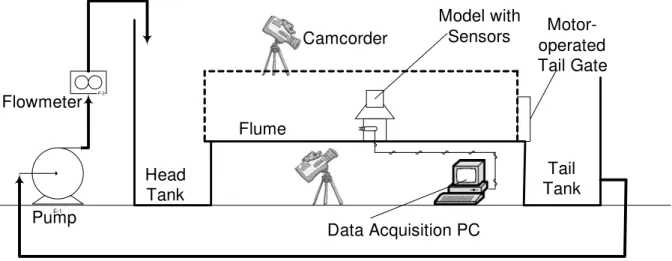
A rectangular flume has been constructed on an elevated platform. Except for a perspex glass replacement for a square window opening to mount the models and facilitate video imaging from underneath, the bottom of the flume is otherwise made of glass laminated over wooden support boards. The sides of the flume are made of perspex glass. A pump discharges the flow into the flume. A schematic diagram is given as figure (8).

E-1 P-1 I-1 P-2 Pump Flowmeter Head Tank

Camcorder _operated Motor-Tail Gate Tail Tank Flume Model with Sensors Data Acquisition PC

Figure 8 : Schematic layout of experiment

The width of the flume has to be so chosen that the edge boundary effects are insignificant. To hold the same, a conservative estimate is to make the middle 1/3rd wide enough to

accommodate the model and accessories. Also, as discussed in the literature study section, a given discharge corresponds to a unique velocity and flow depth in such a channel section, if allowed for free gravity flow. In such a configuration, a change of velocity would be associated with a simultaneous change of flow depth and thus the model has to be moved up or down correspondingly to maintain the wetted depth of the cone. But, if a control mechanism is

introduced, for example a gate at the end of the flume, then the velocity can be altered while still maintaining the desired flow depth. By applying the same technique, a motor-operated tail-gate has been installed at the end of the flume with a variability of its height in the range 0 < h< 0.3

meters. However, this essentially limits the useful flow depth to 0.3 meters while the flow depth cannot be lowered than 0.24 meters for the appreciable submergence of the conical part of the model. So, taking the maximum discharge to be 85 lps. and a minimum flow depth requirement of 0.24 meters, the maximum model velocity would thus be 0.334 m/s. The principal layout measurements are tabulated as follows.

Table 1: Experimental layout principal measurements 1 Flume

Length 6.00 meters

Width 1.06 meters clear flow-bed width

Height 0.65 meters from flow-bed

2 Bed perspex glass window 0.6 × 0.6 sq. meters 3 Tail Gate height

maneuverability

0 < h< 0.3 meters

4 Discharge 0 – 85 liters per second (lps).

5 Model Velocity 0 – 0.334 m/s

2.2 Pier Model

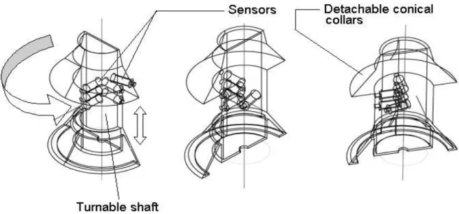
An aluminum model of the pier #31 of the Confederation Bridge has been constructed. As the prototype, it consists of a cylindrical shaft atop a conical base. The conical base is fixed at the bottom to the perspex piece of the flume. The cylindrical shaft consists of slots which can be equipped with pressure sensors or plugged off with ¼ ” MNPT pipe-plugs as required. The shaft is connected to the conical base with an O-ring connection to make the attachment

waterproof. The shaft can be fully rotated in the horizontal plane as well as moved up and down. This enables the measurement of the pressures at different peripheral locations by rotating the shaft and moving it vertically. In order to simulate the prototype, conical collars can be attached to the top portion of the shaft, as shown in figure (9).