Characteristics of Depreciation in Commercial and
Multifamily Property: An Investment Perspective
The MIT Faculty has made this article openly available.
Please share
how this access benefits you. Your story matters.
Citation
Bokhari, Sheharyar, and David Geltner. “Characteristics of
Depreciation in Commercial and Multifamily Property: An
Investment Perspective.” Real Estate Economics 46, 4 (May 2016):
745–782 © 2016 American Real Estate and Urban Economics
Association
As Published
http://dx.doi.org/10.1111/1540-6229.12156
Publisher
Wiley Blackwell
Version
Original manuscript
Citable link
http://hdl.handle.net/1721.1/120153
Terms of Use
Creative Commons Attribution-Noncommercial-Share Alike
Characteristics of Depreciation in Commercial and Multi-Family Property: An Investment Perspective
Sheharyar Bokhari⇤ David Geltner†
This version: March 16, 2014‡
Abstract
This paper reports empirical evidence on the nature and magnitude of real depre-ciation in commercial and multi-family investment properties in the United States. The paper is based on a much larger and more comprehensive database than prior studies of depreciation, and it is based on actual transaction prices rather than ap-praisal estimates of property or building structure values. The paper puts forth an “investment perspective” on depreciation, which di↵ers from the tax policy perspec-tive that has dominated the previous literature in the U.S. From the perspecperspec-tive of the fundamentals of investment performance, depreciation is measured as a fraction of total property value, not just structure value, and it is oriented toward cash flow and market value metrics of investment performance such as IRR and HPR. Depreci-ation from this perspective includes all three age-related sources of long-term secular decline in real value: physical, functional, and economic obsolescence of the build-ing structure. The analysis based on 73,229 transaction price observations finds an overall average depreciation rate of 1.3%/year, ranging from 2.2%/year for properties with new buildings to 0.4%/year for properties with 50-year-old buildings. Apartment properties depreciate slightly faster than non-residential commercial properties. De-preciation is caused almost entirely by decline in current real income, only secondarily by increase in the capitalization rate (“cap rate creep”). Depreciation rates vary con-siderably across metropolitan areas, with areas characterized by space market supply constraints exhibiting notably less depreciation. This is particularly true when the supply constraints are caused by physical land scarcity (as distinct from regulatory constraints). Commercial real estate asset market pricing, as indicated by transaction cap rates, is strongly related to depreciation di↵erences across metro areas.
⇤MIT Center for Real Estate
†Contact author. MIT Center for Real Estate & Department of Urban Studies & Planning
‡The authors gratefully acknowledge data provision and data support and advice from Real Capital
Analytics, Inc. We also appreciate research assistance and useful contributions from Leighton Kaina and Andrea Chegut.
1
Introduction
This paper reports empirical evidence on the nature and magnitude of real depreciation in commercial and multi-family investment properties in the United States. By the term “real depreciation” (or simply, “depreciation”) we are referring to the long-term or secular decline in property value, after netting out inflation, due to the aging and obsolescence of the building structure, apart from temporary cyclical downturns in market values, and even after routine capital maintenance. Such depreciation is measured empirically by an essentially cross-sectional comparison of the transaction prices of properties with build-ing structures of di↵erent ages, controllbuild-ing for other non-age-related di↵erences among the properties and the transactions. In the U.S., most prior studies of depreciation in income-producing structures have been made from the perspective of income tax policy, given that asset value in accrual income accounting in the U.S. is based on historical cost and allows for depreciation to be deducted from taxable income. But considering basic eco-nomics, depreciation is important from an investment perspective apart from tax policy, as depreciation is ubiquitous and significantly a↵ects the nature of property investment performance. Though tax policy considerations certainly are important (including from an after-tax investment perspective for taxable investors), we leave such considerations for another paper.
This investments perspective is the major focus of this paper, though we will also make some observations relevant to the tax policy perspective. From the investment perspective depreciation constrains how much capital growth the investor can expect over the long run, and from this perspective depreciation is measured with respect to total property value not just structure value, and is measured on a cash flow and current market value basis rather than a historical cost accrual accounting basis. In this paper we explore how such depreciation varies with several correlates including metropolitan location, building type, structure age, and market conditions. We also explore the role of income versus capitalization as the source of depreciation.
2
Literature Review
Most of the prior literature on structure depreciation has focused on owner-occupied hous-ing, and as noted, most of the U.S. literature that has focused on depreciation in commercial real estate (income property) has done so from the perspective of taxation policy. An early
and influential example is Taubman and Rasche (1969), which used limited data on build-ing operatbuild-ing expenses to quantify a theoretical model of profit-maximizbuild-ing behavior on the part of building owners to estimate the optimal lifetime of structures and the age and value profile of office buildings, assuming rental revenues decline with building age while operating costs remain constant. The result was a model in which the building structure (excluding land) becomes completely worthless (fit for redevelopment) after generally 65
to 85 years of life, with the rate of depreciation growing with the age of the structure.1
The focus of the analysis was on what sort of depreciation allowances would be fair from an income tax policy perspective.
By the mid-1990s subsequent research led to a consensus that the balance of empir-ical evidence supported the view that commercial structures tend to decline in value in a somewhat geometric pattern (roughly constant rate over time), averaging about 3 per-cent per year (of remaining structure value), though there was some evidence for faster depreciation rates in the earlier years of structure life. (See most influentially Hulton & Wycko↵, 1981, 1996.) In the paper that most influenced subsequent tax policy, Hulton & Wycko↵ (1981) estimated average depreciation rates of approximately 3 percent per year of remaining structure value. With the 1986 tax reform, income tax policy settled on straight-line depreciation methods (which imply an increasing rate of depreciation for older buildings), with the depreciation rate based on 27.5 years for apartments and 31 (subsequently increased to 39) years for non-residential commercial buildings. This has remained a relatively constant and non-controversial aspect of the income tax code since
then.2
Gravelle (1999) reviewed the evidence on depreciation rates for the Congressional Re-search Service and found that rates allowed in current tax law are not too far o↵ from economic reality, if one uses as the benchmark the present value of the allowed
depre-1This is where the depreciation rate is measured as a percent per year of the remaining value of the
structure alone, excluding the land component of the property value. Of course, any model in which the structure becomes completely worthless at a finite age (such as straight-line depreciation) will necessarily tend to have increasing depreciation rates as the structure ages measured as a fraction of the structure value alone excluding land, at least after some point of age. (For example, in the last year of building life, the depreciation rate is by definition 100% of the remaining structure value.)
2Straight-line methods are easy to understand and administer, and can be designed in principle so that
the present value of the depreciation is the same as that of an actual geometric profile of declining building value which might better represent the economic reality. By completely exhausting the book value of the structure at a finite point in time (and hence, exhausting the depreciation tax shields), straight-line methods may tend to stimulate sale of older buildings (so as to re-set the depreciable basis and begin generating tax shields again).
ciation (recognizing that the straight-line pattern is only a simplification). An industry white paper produced in 2000 by Deloitte-Touche studied 3144 acquisition prices of prop-erties held by REITs for which data existed on the structure and land value components separately as of the time of acquisition. The Deloitte-Touche study found approximately constant depreciation rates for acquisition prices as a function of structure age, measured as a percent of remaining structure value, ranging from 2.1%/year for industrial buildings to 4.5%/year for retail buildings (with office at 3.5% and apartments at 4%). However, the study was limited to only buildings less than 20 years old. The Deloitte study also separately estimated depreciation rates for gross rental income, finding rates ranging from 1.7% for office to 2.5% for retail (with industrial at 1.9%, and apartments omitted). Note that, as fractions of pre-existing rent, these depreciation rates would be more comparable to rates based on total property value than just on structure value (Like property value, rents reflect land and location value as well as just structure value.). The working consen-sus apparently persists that, at least for tax policy considerations, commercial structures tend to depreciate in a roughly geometric pattern at typically a rate of 2 to 4 percent of the remaining structure value per year, with apartment structures depreciating slightly faster
than commercial.3
More recent literature is sparse and primarily focused on new empirical data. Fisher et al (2005) used sales of some 1500 NCREIF apartment properties to examine depreciation
in institutional quality multi-family property.4 They conclude that a constant rate of 2.7%
per year of property value including land, or 3.25% of structure value alone, well represents
the depreciation profile for NCREIF apartments.5
There have also been a number of studies of commercial property depreciation in Eu-rope, particularly in the U.K. Many of these studies focus on the investment perspective rather than the tax policy perspective, and they tend to be very applied, industry sponsored reports that use less sophisticated methodologies. In one of the more academic studies, Baum and McElhinney (1997) studied a sample of 128 office buildings in the City of Lon-don and estimated a capital value depreciation rate averaging 2.9%/year as a fraction of total property value (including land), with older buildings (over age 22 years) depreciating
3See United States Treasury (2000).
4NCREIF properties are owned by tax-exempt investors and tend to be at the upper end of the asset
market. The average initial cost in the Fisher et al sample was $17 million.
5NCREIF records indicate that on average almost 20% of apartment property net operating income is
plowed back into the properties as capital improvement expenditures. The depreciation occurs in spite of such upkeep.
less than new or middle-aged buildings. Their study was based on appraised values. More recently, a 2011 study by the Investment Property Forum (IPF), an industry group, exam-ined 729 buildings in the UK that were held continuously over the period 1993-2009. Office buildings were found to experience the highest rate of rental depreciation at 0.8%/year fol-lowed by industrial at 0.5% and retail at 0.3%, all as a fraction of total property value. A comparable IPF (2010) article on office properties in select European cities, estimated depreciation rates that ranged up to almost 5%/year in Frankfurt to no depreciation at all in some cities (such as Stockholm). The IPF studies were based on comparing the rental growth (based on appraisal valuation estimates) of the held properties with that of a benchmark based on a new property held in the same location. However, problems with using valuations and in benchmark selection led Crosby, Devaney & Law (2011) to conclude that these findings are not a good indication of the rates of depreciation in Europe.
3
Investment Perspective on Depreciation
Although tax policy is clearly important, the previous literature’s focus on it may have complicated or omitted some considerations that are more important from a before-tax in-vestment perspective. What we are referring to as the inin-vestment perspective on deprecia-tion is the perspective that reflects the fundamental economic performance of investments. This perspective is the basis on which capital allocation decisions derive their economic value and opportunity cost. In the investment industry profit or performance is measured by financial return metrics such as (most prominently) the internal rate of return and the total holding period return. These metrics are based on market value and cash flow, not on historical cost accrual accounting principles. From the investment perspective there is less rationale for contriving (inevitably somewhat arbitrarily) to separate structure value from land value in investments in real estate assets. At the most fundamental level, real eco-nomic depreciation directly and importantly a↵ects investment returns before, and apart
from, income tax e↵ects.6 Therefore, investors care (or should care) about the granular
characteristics and determinants or correlates of property depreciation, in order to make better property investment and management decisions.
6It is worth noting, as well, that many major investment institutions are tax-exempt (such as pension
and endowment funds). Furthermore, the U.S. is fairly unique in having financial accounting rules based on historical cost asset valuation. In most other countries the type of tax policy considerations that have dominated the U.S. literature on commercial property depreciation are not relevant.
Yet, in practice today it appears that many investors do not think carefully about depreciation in this sense. General inflation masks the existence of real depreciation, and the typical commercial property investment cash flow forecast used in industry (the so-called “pro-forma”) almost automatically and complacently projects rent growth equal to a conventionally defined inflation rate (typically 3%). Unless this assumed general inflation rate is below the realistic inflation expectation in the economy (and usually it is not), then the implication is that investors are typically ignoring the existence of real depreciation, at least in their stated pro-formas. (We shall explore this question further in this paper.)
(a) A Conceptual Framework for Analyzing Depreciation
A careful and complete view of depreciation from the investment perspective must con-sider the causes and correlates of di↵erences in depreciation rates across di↵erent types or locations of properties. Such an investment perspective on depreciation must strive in particular to recognize di↵erences and patterns in the urban economic dynamics of loca-tions of commercial properties. The fundamental economic framework from which to view depreciation from the investment perspective is presented in Figure 1.
Figure 1 depicts a single urban site or property parcel over time, with the horizontal axis representing a long period of time, and the vertical axis representing the money value
of the property asset on the site.7 The top (light) line connecting the U values reflects the
evolution of the location value of the site as represented by the value of the “highest and best use” (HBU) development of the site whenever it is optimally developed or redeveloped (new structure built), an event that occurs at the points in time labeled R. This location value of the site fundamentally underpins the potential long-run appreciation of the property value and the capital return to the investor in the property asset. But the actual market value of the property over time is traced out by the heavy solid line labeled P, which represents the opportunity cost or price at which the property asset would sell at any given time. P declines relative to U due to the depreciation of the building structure on the site. Based on standard cash flow (opportunity cost) based investment return metrics such as IRR or total HPR, it is the combination of the change in location value (U) and the occurrence of structure depreciation which determines the price path of P and hence the capital return
7A very long span of time must be represented, because depreciation is, by definition, a long-term secular
phenomenon, reflecting permanent decrease in building value, and buildings are long-lived, transcending medium-term or transient changes in the supply/demand balance in the real estate asset market.
possibility for the investor over the long run.8
From an investment perspective one can define the “land value” component of the property value in either of two alternative and mutually exclusive ways as indicated in Figure 1. The more traditional conception of land value is labeled L and may be referred to as the “legalistic” or “appraisal” value of the land. It reflects what the parcel would sell for if it were vacant, that is, with no pre-existing structure on it. The second, newer conception of land value comes from financial and urban economics and views the land (as distinct from the building on it) as consisting of nothing more (or less) than the call option right (without obligation) to develop or redevelop the site by constructing a new building
on it.9 This value, labeled C, generally di↵ers from L. The redevelopment call option is
nearly worthless just after a (re)development of the site, because the site now has a new structure on it built to its HBU. But at the time when it is optimal (value maximizing) to tear down the old structure and build a new one, the entire value of the property is just this call option value, the land value. Out-of-the-money call options are highly risky, meaning they have very high opportunity cost of capital (high required investment returns), and the investment returns of options must be achieved entirely by capital appreciation as options themselves pay no dividends. Thus, the call option value of the site tends to grow very rapidly over time between the R points, ultimately catching up with the legalistic or appraisal value of the land.
At the reconstruction points (R) all three measures and components of property value, P, L, and C are the same; the old building is no longer worthwhile to maintain (at least,
given the redevelopment opportunity), so the property value entirely equals its land value.10
8Although it is the total investment return that matters most, including current income (cash flow) plus
change in capital value, there is also interest in breaking out the total return into components, one of which is the current income return or yield rate (net cash flow as a fraction of current asset market value). In such breakout, current routine capital improvement expenditures which are financed internally as plow-back of property earnings are a cash outflow from the property owner, netted out of the income return (i.e., not taken out of the capital return component, from a cash flow perspective). Thus, the investment capital return indicated by the change in P between R points reflects the growth in total property value including (after) the e↵ect of such routine capital improvement expenditures. In the figure 1 model, major externally financed capital improvement expenditures would be considered redevelopments associated with the R points on the horizontal axis.
9The exercise cost (or “strike price”) of the call option consists not only of the construction cost of the
new building plus any demolition costs of the old building, but also includes the opportunity cost of the foregone present value of the net income that the old building could still continue to earn (if any). Thus, for it to make sense to exercise the redevelopment option either the old building must be pretty completely obsolete or the new HBU of the site must be considerably greater than the old HBU to which the previous structure was built.
At that point new capital (cash infusion) in an amount of K is added to the site, as depicted in Figure 1, and this value of K (construction costs including demolition costs) adds to the site-acquisition cost (the pre-existing property value, Old P = L = C) to create the newly redeveloped property value (the new P value = Old P + K) upon completion of the development. The net present value (NPV) of the redevelopment project investment is:
NPV = New P Old P K. In an efficient capital market super-normal profits will be
competed away and this NPV will equal zero, providing just the opportunity cost of its
invested capital as the expected return on the investment.11
The investor’s capital return is represented by the change in the property value P between the reconstruction points in time. The change in P across a reconstruction point R includes new external capital investment (K), not purely return to pre-existing invested financial capital. By definition, property value, P, is the sum of land value plus building structure value. The path of P between reconstruction points therefore reflects the sum of the change in the building structure value plus the change in the land value. The latter reflects the underlying usage value of the location and site as represented by its HBU as if vacant, the U line at the top in Figure 1. Thus, the land value component does not tend to decline over time in real terms in most urban locations, although there certainly are exceptions to this rule. However, the building structure component of the property value will almost always tend to decline over the long run, at least in real terms (net of inflation), reflecting building depreciation. In any case, the extent to which the property value path falls below the location value of the site (U), causing a reduction in the investors capital return below the trend rate in U, is due largely and ubiquitously to building structure depreciation. This is the fundamental reason why, and manner in which, the investor cares about depreciation.
from the value of the land. “Functional obsolescence” refers to the structure becoming less suited to its intended use or relatively less desirable for its users/tenants compared to newer competing structures, for example due to technological developments or changes in preferences, such as need for fiber-optic instead of copper wiring or need for sustainable energy-efficient design. “Economic obsolescence” refers to the phenomenon of the HBU of the site evolving away from the intended use of the structure, the type and scale of the building becoming no longer the HBU for the site as if it were vacant, as for example if commercial use would be more profitable than the pre-existing residential, or high-rise residential would be more profitable than the pre-existing low-rise.
11Note that this zero NPV assumption is consistent with the classical “residual theory of land value”, in
which any windfall in location value accrues to the pre-existing landowner (thus adding to the “acquisition cost” of the redevelopment site, the value of C or L or Old P at the time of redevelopment). However, if the redevelopment is particularly entrepreneurial or innovative, perhaps there will be some Schumpeterian profits for the new developer.
Note that from this perspective the rate at which the building structure itself declines in value due to depreciation is fundamentally ambiguous. This is because building value equals the total property value minus the land value. But there are two very di↵erent yet fundamentally equally valid ways to define and measure land value, the legalistic or appraisal perspective (L) and the economic or functional call option perspective (C). The
structure value component (labeled S in Figure 1), can be defined either as P L or P
C. Thus, the rate of depreciation expressed as a fraction of building structure value is ambiguous from the investment perspective. However, depreciation measured as a fraction
of total property value, P, is not ambiguous.12 Therefore, from the investment perspective
(as distinct from the tax policy or accrual accounting perspective), it is more appropriate to focus on depreciation relative to total property value including land value (P) rather than only relative to remaining structure value (S). We will adopt this approach for the remainder of this paper.
Finally, given that land generally does not depreciate, an implication of this framework is that we should expect newer properties to depreciate at a faster rate since land value is a smaller proportion of the total property value of a new building. This also suggests that depreciation rates may vary across metropolitan areas as di↵erent cities have di↵erent scarcity of land, and therefore, di↵erent land value proportions of total property value. We test both these hypotheses in our subsequent empirical analysis.
(b) Source of Depreciation: Income or Capitalization?
It is of interest from an investment perspective to delve deeper into the depreciation phe-nomenon and explore how much depreciation is due to changes in the current net cash flow the property can generate as it ages versus how much is due to the property asset market’s reduction in the present value it is willing to pay for the same current cash flow as the building ages. This latter phenomenon is sometimes referred to as “cap rate creep”. Such
12It is worth noting that, apart from the conceptual problem, measuring depreciation as a fraction of
structure value (S) is also difficult to estimate empirically. This is because, compared to quantifying the total property value, P, it is usually relatively difficult to quantify either L or C for a given property at a given time. While appraisers or assessors sometimes estimate the value of L, such valuations are only estimates, and are often crude and formulaic. In built-up areas there is often little good empirical evidence about the actual transaction prices of comparable land parcels recently sold vacant. And land value estimates can be circular from the perspective of quantifying structure depreciation, as the land value may be backed out from property value minus an estimate of depreciated structure value, meaning that for purposes of empirically estimating structure depreciation we get an estimate of depreciation based on an estimate of depreciation!
an understanding could improve the accuracy of investment return forecasts, and possibly
improve the management and operation of investment properties.13
By way of clarification and background, consider the fundamental present value model of an income property asset:
Pi,t = 1 X s=t+1 Et[CFs] (1 + ri,t)s t (3.1)
where Pi,t is the price of property i at time t; Et[CFs] is the expectation as of t of the
net cash flow generated by the property in future period s; and ri,t is the property asset
market opportunity cost of capital (OCC, the investor’s required expected total return) for property i as of time t. With the simplifying assumption that the expected growth rate
in the future cash flows is constant (at rate gi,t) and the property resale price remains a
constant multiple of the current cash flow, (3.1) simplifies to the classic “Gordon Growth Model” of asset value (GGM), which is a widely used valuation model in both the stock
market and the property market:14
Pi,t =
Et[CFs]
ri,t gi,t
(3.2) With the slight further simplification that the net operating income approximately equals
the net cash flow (NOIi,t ⇡ Et[CFs]),15 this formula provides the so-called “direct
capi-talization” model of property value which is widely used in real estate investment:
Pi,t =
N OIi,t
ki,t
(3.3)
13For example, there might be things the investor could do to mitigate the decline in net cash flow,
whereas there might be less that can be done to influence caprates.
14Clearly the GGM is a simplification of the actual long-term cash flow stream as modeled in Figure 1.
But the GGM is widely used and its simplification is relatively benign for our purpose, which is only to explicate the basic roles in property depreciation of the two factors, current net cash flow and asset market capitalization.
15The di↵erence between N OI and CF is the routine capital improvement expenditures: CF
t= N OIt
CIt. Although this di↵erence does not matter for our purpose in this paper, it is of interest to note that
among properties in the NCREIF Property Index, the historical average capital expenditure (CI) is over 2% of property value (including land value) per year. Deloitte-Touche (2000) reports that U.S. Census data indicates overall post-construction capital improvement expenditures on buildings is approximately 40% of the cost of new construction. (If the average building is somewhat more than 20 years old, this would be roughly consistent with the NCREIF 2%/year rate.) The Deloitte-Touche study also conducted a survey which suggested that capital expenditures may often exceed 5% of structure value per year. (If structure value is on average halfway between 80% and 0% of total property value, then this too would be roughly consistent with the NCREIF data.) However, the D-T survey was very limited.
where ki,t = ri,t gi,t is the capitalization rate (“cap rate” for short) for property i as of
time t. The property value equals its net operating income divided by its cap rate. Thus, if the property real value tends to decline over time with depreciation, due to the aging of the building, then such value decline may be (with slight simplification) attributed either to a decline over time in the real NOI that the property can generate, or to an increase over time in the cap rate that the property asset market applies to the property as it ages, or to a combination of these two sources of present value. To the extent depreciation results from an increase in the cap rate with building age (“cap rate creep”), this could result either from an increase in the OCC or from a decrease in the expected
future growth rate, gi,t, or a combination of those two. In the present paper we will not
attempt to parse out this OCC versus growth expectations breakout. We content ourselves with exploring the question of how much of the depreciation in P is due to the NOI and how much is due to k. To answer this question, we will estimate the e↵ects of depreciation on both property value and on cap rates. The di↵erence between the total depreciation and e↵ect of the cap rate creep will be attributable to NOI depreciation. We now turn to outlining our empirical model.
4
The Hedonic Price and Cap Rate Models
In this section, we outline our approach for estimating the e↵ects of depreciation on both total property value and the property cap rate. Following in the tradition of depreciation estimation modeling, the approach known as “used asset price vintage year” analysis is applied to quantify real depreciation. This involves an essentially cross-sectional analysis of the prices at which properties of di↵erent ages (defined as the time since the building was constructed) are transacted, controlling for other variables that could a↵ect price either cross-sectionally or longitudinally. This is estimated via the hedonic price model given in equation (4.1) ln(pi,t) = H X h=1 AAh,i,t+ J X j=1 XXj,i,t+ M X m=1 MMm,i,t+ T X s=1 TTs,i,t+ ✏i,t (4.1) where,
• pi,t is the price per square foot of property sale transaction i occurring in year t.
• Ah,i,t is a vector of H property and location characteristics attributes for property
sale transaction i as of year t.
• Xj,i,tis a vector of J transaction characteristics attributes for property sale transaction
i as of year t.
• Mm,i,t is a vector of fixed-e↵ects dummy variables representing M metropolitan
mar-kets for property sale transaction i as of year t
• Ts,i,t is a vector of s = 1,2,...,T time-dummy variables equaling one if s = t and zero
otherwise (for property sale transaction i as of year t).
The Ah property and location characteristics in the model include, most importantly,
the property age in years since the building was constructed and age-squared, but also include the natural log of the property size in square feet, dummy variables for property usage type sector (office, industrial, retail, or apartment), and a dummy variable flagging
whether the property is in the central business district (CBD) of its metro area. The Xj
transaction characteristics include an indicator of seller type, a dummy variable to control whether the sale was in distress, a dummy variable to indicate if the buyer had a loan that was part of a CMBS pool, as well as flags to indicate whether the transaction was a sale-leaseback or whether the property had excess land available (was not fully built out). We also estimate a hedonic model of the cap rate that can, similar to the analysis of property price, quantify how the cap rate is a function of the age of the property’s building structure (holding other characteristics constant). This cap rate model can then be combined with the hedonic price model to derive how much of the overall depreciation in the property value is due to depreciation in the property net operating income and how much is due to change in the cap rate.
Our hedonic cap rate model is very similar to our hedonic model of property price in (4.1) except that we replace the dependent variable with a normalized construct of the property’s cap rate at the time of sale instead of the property price. The normalized cap rate is the di↵erence between the property’s cap rate minus the average cap rate prevailing in the property’s metropolitan market (for the type of property) during the year of the transaction. This normalization controls for systematic di↵erences in cap rates
across metropolitan areas, as well as for cyclical and market e↵ects on the cap rate.16 The
16Alternatively, cap rates on the left hand side and interacted dummies between MSA and time would
normalized cap rate thus allows the individual property di↵erences in cap rates that could be caused by the age of the buildings to be estimated in the model below:
CapRatei,t= H X h=1 AAh,i,t+ J X j=1 XXj,i,t+ M X m=1 MMm,i,t+ T X s=1 TTs,i,t+ ✏i,t (4.2)
5
Data
This study is based on the Real Capital Analytics Inc (RCA) database of commercial
property transactions in the U.S.17 RCA collects all property transactions greater than
$2,500,000, and reports a capture rate in excess of 90 percent. Properties smaller than $2.5M are often owner-occupied or e↵ectively out of the main professional real estate in-vestment industry. We believe the data represent a much larger and more comprehensive set of investment property transactions than prior studies of depreciation. The present analysis is limited to the four major core property sectors of office, industrial, retail, and apartment. The study dataset consists of all such transactions in the RCA database from 2001 through the first quarter of 2013 and which pass the data quality control filters and for which there is sufficient hedonic information in the RCA database, 73,229 transactions in
all.18 This includes 55,913 non-residential commercial property sales and 17,316 apartment
property sales. A subsample of 55,316 transactions are located in the top 25 metropolitan
area markets which are studied separately.19 21,910 sales have, in addition to sufficient
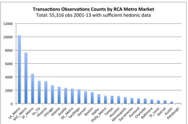
he-donic data, also reliable information about the cap rate (as defined in section 3). This cap rate subsample will be used in subsequent analysis of the cap rate creep. Table 1 presents the summary statistics for the overall dataset. The average age of the properties in our sample is 29 years. The data are fairly equally distributed across the four core property types. The seller types are broadly categorized as Equity, Institutional, Public, Private, User and CMBS Financed, of which Private constitutes about 67% of the data. Figure 2
identical results, not surprisingly.
17In general from here on, unless specified otherwise or it is clear from the context, we will use the term
“commercial” property to refer to all income-producing property including multi-family apartments.
18We drop sales that were part of a portfolio sale to avoid an uncertain sale price for a property within
the portfolio. We also drop properties for which the sale price was not classified as confirmed by RCA’s standards and if they were older than 100 years.
19RCA has their own definition of metropolitan areas which di↵er slightly from the U.S. Census definitions
and conform better to actual commercial property markets. We refer to these as “RCA metros” or “Metro Markets.”
shows the number of observations in each of the top 25 RCA Metro Markets. The sample sizes range from 10,246 transactions in Metro Los Angeles down to only 208 in Pittsburgh. It should also be noted that the data contains two fields which can relate to the ef-fective “age” of the property. One field indicates the year of initial construction of the building, the other field attempts to indicate the year of any major renovation. Because the renovation field is not viewed as reliably or consistently filled in, we have ignored it in the results reported herein, basing property age only on the year of original construc-tion of the building. However, this means that the depreciaconstruc-tion we find will to a small extent reflect not only the e↵ect of routine capital improvements and upkeep, but also occasionally of more substantial renovations. This will tend to make our results about the magnitude of depreciation conservative in the sense of tending to understate the true rate
of depreciation.20
6
Empirical Analysis
(a) Depreciation Magnitude and Age Profile
The first set of results is based on the hedonic price model in (4.1), run on the entire 73,229 US transaction sample, and focuses on the overall rate of depreciation and its profile over time. Column (1) in Table 2 presents the regression results. The variables of interest, both Age and Age-squared, are highly significant, with the coefficient on Age being negative and that on Age-squared being positive; a convex quadratic function. Thus, the property value tends to decline in real terms with building age, but at a declining rate. To check the robustness of this result, column (2) of Table 2 shows an alternative specification where instead of Age and Age-squared, we use categorical age dummy variables, with the omitted group being properties less than 10 years old. We again find here that relative to newer properties, older properties depreciate at a slower rate. For instance, relative to the base age group, properties in the 10 to 20 years age group will have depreciated on average approximately 28% of their property value, whereas properties in the age 20 to 30 year group will have depreciated by 42%, only a further 14%; highlighting a slower rate of
20Analysis of the data dropping any observations with renovation dates di↵erent from the initial
construc-tion date suggests that depreciaconstruc-tion would be approximately 20 basis-points per year greater than what is reported in this paper.
depreciation when a property enters the latter age group.21 Although not important from
the investment perspective (as distinct from the tax policy perspective), it is worth noting that the result that properties with newer buildings depreciate at faster rates than those with older buildings on them, could conceivably be consistent with a geometric building value function in which the rate of depreciation is constant as a fraction of remaining building value but the building value component is a declining fraction of the total property value as the land value component assumes a larger share of the remaining property value. (More on this shortly.)
Using the quadratic specification as the more parsimonious model, we note that, since the Age-squared coefficient is significant, we cannot completely quantify the average rate of property depreciation using only the coefficient on Age. The property’s depreciation rate is a function of the age of the building on the property. To account for this, we adopt the following approach to quantifying a summary metric for depreciation rate. We model the depreciation rate (using the Age and Age-squared coefficients) for all building ages from 1
to 50 years old.22 We then take, as our summary measure of average depreciation rate, the
equally-weighted average rate across the 50 year horizon. (That is, each of the 50 years’ rates counts equally. This average is normally very similar to the depreciation rate of a 25
year old building.23) Thus, in e↵ect, this is a summary depreciation metric that holds the
age of the building structure constant across comparisons, at the time-weighted average
21Note that the coefficient on the oldest age group (buildings over 50 years in age) is 0.47 compared
to 0.50 for the next-oldest group (30-50 years old), indicating a slight upturn in property value for very old buildings. This also is consistent with a convex quadratic model, and probably reflects a leveling o↵ of property value as a function of building age when very old structures are present. By then the property value may consist largely of land value, resulting in practically no further depreciation. It is also possible that there is a slight survivorship bias as structures of historical value or of particularly prized aesthetic value no doubt have a greater propensity to survive into the oldest age group. Note, however, that from the investment perspective, there is no censorship of our sample, per se, as it is the investor (property owner) who decides if and when to demolish the existing structure, and such decisions are made to maximize profit. In the context of the model in Section 3, the demolition decision reflects the exercise of the redevelopment call option, which does not by any means imply an exhaustion of property value. (The investment perspective takes the investor and the property asset as its focus, not the pre-existing building structure alone.)
22These depreciation rates are derived from the regression results by exponentiating the di↵erence in the
regression-predicted log values of the property at the reference age compared to one year younger (and subtracting from one). Recognizing that the non-age-related regressors cancel out, the computation is as follows:
1 e[AgeCoef f⇤Age+AgeSquaredCoeff⇤(Age)2 [AgeCoef f⇤(Age 1)+AgeSquaredCoeff⇤(Age 1)2]]
depreciation rate over a 50-year building life horizon.
For the national sample, this gives an average real depreciation rate of 1.26%/year of property value (including land). The depreciation rate declines from 2.15%/year for a property with a new building down to 0.37%/year for a property with a 50-year old building (see Figure 3). At first glance, these depreciation rates appear to be smaller than what was reported in earlier studies in the U.S., such as the Hulton-Wycko↵ (1981) and Deloitte-Touche (2000). But those studies were quoting rates as a fraction of remaining estimated structure value, not total property value which is our focus.
We have noted in Section 3 that from the investment perspective it is less important to attempt to quantify depreciation as a fraction of only structure value. Nevertheless, to compare our results with the previous U.S. depreciation literature, it may be of some interest to make some observations in that regard. Suppose, for example, that structure value declines from 80% to 0% of total property value over the lifetime of the structure, and on average it is at the midpoint of that decline in percentage terms (40% of property value). Then to convert our empirical depreciation findings to an average fraction of remaining structure value we would magnify the rates reported here by a factor of 2.5. In this case our overall average rate as a fraction of structure value would be 1.26%/0.40 = 3.15%, which would be roughly consistent with the previous studies’ findings. On the other hand, suppose we take a straight-line model of building value holding land value constant. Starting from a building value of 80 and land value of 20 for a total property value of 100, the property value declines linearly to a value of 20, all land, at the end of the building’s life. In that case, midway through the life the building is worth 40, the land always 20 for a total property value of 60, so the building still amounts to 67% of the property value (40/60) at the midlife point. In that case, we would magnify our property-based percentage rates only by a factor of 1.5 instead of 2.5, suggesting an average annual depreciation rate of 1.9% of structure value, a bit less than what the earlier studies reported. Finally, to illustrate the other extreme, suppose we ask what annual depreciation rate as a fraction of remaining structure value will cause our empirical findings about the total property value quadratic depreciation function to be consistent with an approximately constant geometric depreciation of the structure such that the property value is entirely land after about 50 years. This would require that the land fraction at the time of (re)development be nearly half the total property value, which gives a nearly constant structure depreciation rate of approximately 4%/year, which is a bit higher than most of the earlier studies found based on estimated building value and simple geometric depreciation. Thus, it is perhaps
not possible to make any strong claim about whether our findings are greater or lesser than what is implied by earlier studies, in part because the definition and measurement of remaining structure value is a rather imprecise exercise (as distinct from total property value as indicated by transaction price).
In Table 3, we run separate regressions for the 4 core property types. We find (consis-tent with the national aggregate results) signs and significance for the Age and Age-squared variables across all property types. In the case of non-residential commercial real estate, office and retail properties depreciate the fastest at similar rates, while industrial depre-ciates the slowest (at least until buildings become very old). In Figure 4, we lump all the non-residential commercial property sectors together and break out the analysis sep-arately for apartments and non-residential commercial properties. It is not clear a priori why apartment properties should depreciate at di↵erent rates than commercial property, but tax policy has long di↵erentiated them (possibly for political reasons). In fact, we see that apartments do on average depreciate slightly faster than non-residential commercial properties, holding age constant. The average depreciation rate (as defined previously) for apartments is 1.71%/year and the average rate for non-residential income properties is 1.30%/year. In the case of apartments the rate declines from 2.91%/year with a new build-ing to 0.49%/year with a 50-year old buildbuild-ing. In the case of non-residential commercial the rate declines from 2.33%/year new to 0.26%/year at 50 years.
In summary, our aggregate-level findings suggest depreciation rates that average clearly over one percent per annum as a fraction of total property value (including land). Com-pared to the previous literature, our estimates are based on actual transaction prices rather than building structure value estimates, and are based on a much larger and more compre-hensive property sample. Depending on how one adjusts or estimates remaining structure value, the rates we find could be consistent with the earlier findings, although there is some suggestion that the depreciation rates in our data may be a bit less than the earlier studies reported (based on the middle assumption noted above, multiplying our rates by a factor of 1.5). We find clear evidence that properties depreciate slower as buildings age. There is also clear evidence that apartment properties depreciate faster, but only slightly faster, than non-residential commercial properties.
(b) Estimation of Cap Rate and NOI E↵ects on Total Depreciation
In order to estimate how much property value depreciation would result purely from cap rate creep, and how much from NOI decline, we estimate the hedonic price and cap rate models (equations (4.1) and (4.2) respectively) on the same transaction subsample for which we have cap rate data available. These regressions are shown in columns (1) and (2), respectively, of Table 4. We first compute the total depreciation in property value from the age coefficients in the price model (column (1) of Table 4), much as described in the previous section. We next compute how much decline in property value with building age would result purely from the increase in the cap rate due to age as implied by the age coefficients in the cap rate model (column (2) of Table 4), holding the property net operating income constant. The di↵erence between the total depreciation and the pure cap rate creep depreciation presumably is attributable to NOI depreciation.
The result of this analysis is shown in Figure 5. It can be seen that almost all of the property value real depreciation results from the decline in the real NOI and very little from cap rate creep. Using our previously defined average-age metric for the summary depreciation rate, the overall average depreciation rate in the subsample is 1.62%/year, while the average depreciation rate due solely to cap rate creep is only 0.11%/year. The implication is that the NOI source of depreciation accounts for 1.51%/year or 93% of all the depreciation. This implies that the conventional approach in current investment industry practice in commercial property pro-formas of forecasting rent and cash flow growth at a standard 3% rate (presumably equal to inflation but in reality if anything slightly greater than inflation in recent years) is substantially biased on the high side, especially for newer buildings.
Because discounted cash flow (DCF) analyses of such pro-forma cash flow forecasts must of necessity arrive at a present value for the property approximately equal to the current market value of the property, this implies that the discount rate employed in such analyses must be substantially greater than the actual opportunity cost of capital. In other words, the discount rate typically employed in micro-level real estate investment analysis in the industry today is substantially greater than the actual realistic expected total return on the investment.
The dominance of net income and the space market as the fundamental source of property value in real depreciation is interesting in view of the fact that changes in capi-talization, in the asset market’s opportunity cost of capital or future growth expectations,
have been found to play a major and perhaps even dominant role in short to medium-term
movements in property value.24 But depreciation is a very long-term secular phenomenon,
and it makes sense that it would largely reflect underlying fundamentals.
Related to this point, we examined whether there is any evidence that depreciation was di↵erent during the boom (sometimes referred to as the “bubble”) in the commercial property market in the middle of the last decade. We divided the transaction sample into two subsamples. During the three boom years of 2005-07 (inclusive), we have 23,885 sales; and during the other nine years of the sample (2001-1Q2013 excluding 2005-07) we have 49,344 observations. Although we do find that during the boom years the depreciation rate was statistically significantly less than during the other years, the di↵erence is very small and lacks economic significance. The average di↵erence in the implied depreciation rate was less than 0.2%/year, and the lifetime profile di↵erence is shown in Figure 6.
(c) Depreciation and Metropolitan Location
We noted previously that real depreciation is a phenomenon of decline in the value of the building structure on the property, as land generally does not depreciate (or not as much or as relentlessly). This probably largely accounts for why the rate of depreciation is greater in properties with newer buildings. This also strongly suggests that property depreciation rates may vary across metropolitan areas, as di↵erent cities have di↵erent scarcity of land and di↵erent land value proportions of total property value. To analyze this issue, we estimated the hedonic price model in (4.1) separately for the top 25 Metro Markets (see again Figure 2 for the same sizes in each metro).
Figure 7 shows the resulting estimated coefficients on the Age variable in (4.1), in terms of absolute value (higher value is faster depreciation). Both the Age and Age-squared coefficients are statistically significant for all 25 Metro Markets. The Figure ranks the metros from greatest (fastest) to lowest (slowest) depreciation (based on the Age coefficient) and shows the 2-standard-deviation confidence bounds around the Age coefficient estimate in each metro. However, recall that the Age coefficient by itself is not the complete story about depreciation, as the e↵ect of the Age-squared coefficient must also be considered, which makes the property depreciation rate a function of building age. Table 5 therefore shows for each metro the implied depreciation rates as a function of building age, as well as the time-weighted average summary metric for each metro (which e↵ectively compares
across metro holding building age constant). Finally, Figure 8 depicts some representative age/value profiles for several major metropolitan areas, providing a visual impression of how both the average depreciation rate and the age profile of the depreciation can vary across select metropolitan areas.
The extent of variation across metropolitan areas is striking. For the age-constant sum-mary metric, the average depreciation rate for all income-producing commercial property ranges from over 2.6%/year in Dallas down to less than 0.4%/year in Los Angeles. The age profile also can vary greatly, with a few metros apparently exhausting the property
depreciation just prior to 50 years of building age.25 This probably does not generally
reflect an historic building or “vintage e↵ect” as has been sometimes found for
single-family houses.26 And income-producing properties, essentially capital assets traded in the
investments industry, are probably not very susceptible to architectural style vintage year preference e↵ects like houses may be. Rather, the exhaustion of property depreciation probably suggests rapid economic obsolescence in a dynamic metropolitan area where the highest and best use (HBU) of locations has been rapidly changing over the past couple of generations.
On the other hand, metro areas that show little depreciation right from the start, even when buildings are new, may reflect systematically higher land value proportions of total property value, even when the buildings are new. This may reflect land scarcity. Figure 9 explores this issue by regressing the metro areas’ depreciation rates onto the
Saiz measure of metro area real estate supply elasticity.27 The Saiz elasticity measure is
based on both regulatory and physical land supply constraints on real estate development, which Saiz has shown are major determinants of overall real estate development supply elasticity. Thus, the Saiz elasticity measure should be highly correlated (negatively) with land value and the land value fraction of total development costs (and therefore, with the average land value fraction of total property value). Metro Markets with higher Saiz elasticity measures probably tend to have lower land values. Figure 9 indeed reveals a strong positive relationship between depreciation and the Saiz elasticity. Metro areas that tend to have more elastic supply of real estate by the Saiz measure (which probably have
25The most extreme case is the South Florida Metro Market (Miami-Ft.Lauderdale-W.Palm Beach),
which actually indicates a minimum property value at building age around 40 years.
26See Clapp & Giacotto (1998), who document that home buyers may develop preferences for certain
vintages of housing construction.
27Figures 9, 10, 11 and 12 show results for 24 instead of 25 metro areas because at present there is no
lower land costs resulting in building value being a larger share of total property value) are
associated with faster depreciation, especially in the early years of building life.28 We see
the opposite in metros that have the lowest Saiz elasticities.29
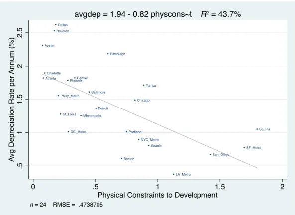
In Figure 10, we regress MSA depreciation rates against the physical land constraint component of Saiz’s elasticity measure. The physical land constraint measure is a sum of various geographical constraints within a 50km radius from the center of an MSA. These constraints include the share of land area that’s at more than a 15% slope, or if it is under open water or wetlands, or generally not available for development. The figure shows that depreciation rates are lower in MSAs where there are greater (higher value) physical constraints to development. This again is consistent with the view that land value proportions of total property value would be higher in such MSAs and therefore, depreciation in the structure would be a smaller percentage of total property value.
In Figure 11, we regress MSA depreciation rates against the Wharton Land Regulation Index (WLRI, also a component of Saiz’s elasticity measure). In the Figure, higher values reflect greater regulatory constraints and we see a negative relationship between average depreciation rates and the WLRI. However, the relationship between depreciation and regulatory constraints in Figure 11 is weaker than the relationship between depreciation and physical land constraints in Figure 10. Onerous regulations constrain development without adding to land value (they don’t cause land scarcity per se but merely an increase in development costs), while physical land constraints should cause land scarcity and higher land costs. In a simple regression of average MSA depreciation rates onto the Saiz physical land constraints measure and the WLRI, we find that the physical land constraints measure has greater explanatory power than the WLRI measure. The physical land constraint measure has a bigger coefficient ( 0.68) and higher statistical significance (at 1% level) than WRLI, which has a coefficient of 0.28 and is only statistically significant at the 10% level. Physical land constraints alone can explain over 44% of the variation in average depreciation rates across MSAs while adding WRLI only marginally increases the explained variation to 52%. Thus, low depreciation is more associated with physical land constraint
28As noted, lower depreciation as a fraction of property value in later years (older buildings) in metro
areas with rapid initial depreciation rates could reflect exhaustion of building value due to widespread economic obsolescence of structures reflecting very dynamic metropolitan growth. This may be seen in the di↵erence between the 1-yr-old minus 50-yr-old depreciation rates in cities such as Dallas, Denver, Phoenix, Atlanta, Austin, Tampa and South Florida.
29Most notably the West Coast metros (LA, SF, SD, Seattle, Portland) and major North Atlantic metros
than with regulatory constraints.
The analysis in Figures 9, 10 & 11 explores a major cause of the cross-section of metropolitan depreciation rates in commercial property. On the other hand, the analysis in Figure 12 explores a major e↵ect of this variation in depreciation rates. Figure 12 regresses the average cap rates of property sale transactions onto the average depreciation rates across the Metro Markets. As noted in our derivation of the direct capitalization formula for property value in Formula (3.2) in Section 3, cap rates can be viewed as reflecting essentially or primarily the current opportunity cost of capital (the investors’ expected
total return, ri,t) minus the long-term expected growth rate in property value (what we
labeled gi,t, which fundamentally and primarily reflects the long-term growth in property
net income). Clearly the long-term growth rate strongly reflects the property depreciation rate that we have been estimating. Therefore, we should expect property transaction prices, as reflected in their cap rates, to be partially and importantly determined by depreciation expectations. Thus, the dispersion in cap rates should be correlated with the dispersion in depreciation rates across Metro Markets. Figure 12 shows that this is exactly what we find. The relationship is strongly positive and statistically significant.
However, the cap rate/depreciation relationship in Figure 12 is less than a one-to-one correspondence (slope is less than 1.00). If cap rates were completely determined by the
ri,t gi,t relationship, and if gi,twere completely determined by depreciation (growth is the
negative of depreciation), then we would expect the estimated slope line in Figure 12 to be closer to 1.00. Instead, the slope is just under 0.5. Apparently cap rates are a bit more
complicated than ri,t gi,tand/or the growth that matters to investors is more complicated
than just the long-term depreciation that characterizes the metro area.
Nevertheless, Figure 12 suggests that the type of depreciation we are measuring is important for investors, as it should be. This finding suggests some nuance on the point we made previously that in current industry practice the routine cash flow forecasts in individual property investment DCF valuations seem to ignore real depreciation and the di↵erences in depreciation across metro areas. While this is true of the cash flow forecasts in the numerators of the DCF present value analyses, the discount rates applied in the denominators are more flexible and are used to bring those cash flow forecasts in the numerators to a present value that coincides with current asset market valuation which does, apparently, reflect sensitivity to di↵erences in growth and depreciation across metro areas. In other words, the discount rates used by investors must tend to be smaller in metro areas with less depreciation, and larger in those with greater depreciation. An e↵ect
which actually, realistically exists in the numerators (cash flows) is instead applied in the denominators (discount rate). As the discount rate is, in principle, the investor’s going-in expected return, this suggests a lack of realism in these expected returns, both on average in general, and relatively speaking cross-sectionally, particularly in high depreciation Metro
Markets such as many in the South and interior Sun Belt.30
7
Conclusion
In this paper we have analyzed the wealth of empirical data about U.S. commercial invest-ment property contained in the RCA transaction price database in order to characterize the nature and magnitude of real depreciation. We introduce and explicate what we call the investment perspective for this analysis, which di↵ers from that of the income tax policy oriented studies that have dominated most of the past literature in the U.S. The investment perspective is based on before-tax cash flow and market value metrics such as the IRR and the holding period total return that are prominent in the financial economics field, instead of on the historical cost accrual accounting perspective that underlies IRS tax policy in the U.S. Given our investment perspective, we focus on depreciation as a fraction of property total value (including land value), although we make some observations about building value fractions in order to place our empirical findings in comparison to results reported in earlier literature.
To briefly summarize our empirical findings about depreciation in income property viewed from the investment perspective, we see first that depreciation is significant. With average rates well over 100 basis-points per year, often over 200 bps in newer properties, depreciation has an important impact on realistic expected returns and property investment values. Furthermore, depreciation varies in interesting ways. It tends to be greater in younger properties (those with more recently constructed buildings). This probably largely reflects the relative share of land value and building structure value in overall property value, as land does not tend to depreciate. Holding building age constant, depreciation tends to be slightly greater in apartment properties than in non-residential commercial
30This lack of a realistic correspondence between the implied expected returns and the realistic expected
returns does not necessarily imply that asset mispricing exists. Asset prices reflect supply and demand for investment assets, and could rationally reflect risk and return preferences and perceptions. For example, Dallas properties may realistically provide less expected return than is suggested by the discount rates employed in their DCF analyses, but they also may present less risk than would warrant expected returns as high as the discount rates.
properties. Depreciation varies importantly across metropolitan areas. We see that metros with lower development supply elasticity, especially places with physical land constraints such as the large East and West Coast metropolises, have lower depreciation rates. Places with plenty of land and less development constraints (higher supply elasticity) have higher average depreciation (holding building age constant). In some cases, notably in the South and interior Sun Belt metropolises, depreciation exhausts building values within around 50 years or perhaps even less. This may be due to dynamic growth in the metro area causing more widespread economic obsolescence. We also confirm that investment property asset prices do significantly reflect the di↵erences in depreciation rates across metropolitan areas (as they should with rational asset pricing), though depreciation can only explain about half of the cross-sectional di↵erences in cap rates.
Finally, we have seen that real depreciation is largely caused by (or reflects) real de-preciation in the net operating income (NOI) that the property can generate, rather than by “cap rate creep” (increasing property cap rate with building age). Depreciation is a long-term secular phenomenon, so it makes sense that it would largely reflect property value fundamentals. This finding, combined with the magnitude of real depreciation that we find, strongly undercuts the realism in the typical prevailing industry practice of au-tomatically forecasting a rental growth rate of 3%/year in most cash flow pro-formas and DCF present value analyses of individual property investments.
References
Baum A. and McElhinney A., The causes and e↵ects of depreciation in office buildings: a ten year update. RICS - Royal Institution of Chartered Surveyors. London. 1997
Clapp, John M. and Giaccotto, Carmelo, Residential Hedonic Models: A Rational Expec-tations Approach to Age E↵ects, Journal of Urban Economics, 1998, 44, 415-437
Crosby, N., S. Devaney and V. Law, Benchmarking and valuation issues in measuring depreciation for European office markets. Journal of European Real Estate Research, 2011, 4: 1, pp 7 -28
Geltner, D. and Mei, J., The present value model with time-varying discount rates: Impli-cations for commercial property valuation and investment decisions, Journal of Real Estate Finance and Economics, 1995, 11:2, 119135.
Gravelle, J.G., Depreciation and the Taxation of Real Estate. Congressional Research Service, Washington, DC, 1999.
Hulten, C. R. and F. C. Wyko↵, The Estimation of Economic Depreciation Using Vintage Asset Prices: An Application of the Box-Cox Power Transformation, Journal of Economet-rics, 1981, 36796.
Hulten, C. R. and F. C. Wyko↵, Issues in the Measurement of Economic Depreciation: Introductory Remarks, Economic Inquiry, 1996, 34:1, 1023.
IPF, Depreciation of Office Investment Property in Europe, Investment Property Fo-rum/IPF Educational Trust, London. 2010.
IPF, Depreciation of Commerical Investment Property in UK, Investment Property Fo-rum/IPF Educational Trust, London. 2011
Plazzi,A., W.Torous and R.Valkanov. Expected returns and expected growth in rents of commercial real estate. Review of Financial Studies 23(9): 3469-3519.
Sanders, H. and W., Randall, Analysis of the economic and tax depreciation of structures, Deloitte and Touche LLP, Washington DC June 2000
Taubman, P. and R. H. Rasche, Economic and Tax Depreciation of Ofce Buildings, National Tax Journal, 1969, 22, 33446.
U.S. Treasury Department, Report to the Congress on Depreciation Recovery Periods and Methods, 2000.
Property $ Value Components
Time
R R R R
R = Construction / reconstruction points in time (typically 30-100 yrs between) U = Usage value at highest and best use at time of reconstruction
P = Property value S = Structure value
L = Land appraisal value (legal value)
C = Land redevelopment call option value (economic value) K = Construction (redevelopment) cost exclu acquisition cost
U U U U P P P P C S L L K K The$component$of$total$property$value$(P)$attributed$to$the$building$structure$equals$the$component$ not$attributed$to$land$value.$There$are$two$ways$to$conceptually$define$land$value:$“L”$is$the$ legal/appraisal$definition$(value$of$comparable$vacant$lot);$“C”$is$the$economic$definition$(value$of$the$ redevelopment$call$option).$In$the$graph$below,$S$=$PHC.$But$most$practical$applications$use$the$legal$ definition$of$land$value,$and$S$=$PHL.$Depreciation$results$from$any/all$of$three$forms$of$obsolescence:$ (i)$Physical$(wearing$out,$more$expensive$maintenance),$(ii)$Functional$(components$&$design$no$ longer$optimal$for$the$intended$use),$&$(iii)$Economic$(intended$use$no$longer$optimal$for$the$site).
0" 2000" 4000" 6000" 8000" 10000" 12000" LA_Me tro" NYC_Me tro" SF_Me tro" So_F la" Phoen ix" Chicag o" Atlan ta" Sea> le" DC_Me tro" SanDie go" Denv er" Bosto n" Dallas "" Philly _Metro " Tampa"Houston
" Minn eapoli s" Sacram ento" Portl and" Charl o>e" BalJm ore" St_Lou is" Detro it" AusJ n" Pi>sb urgh" Transac'ons)Observa'ons)Counts)by)RCA)Metro)Market) Total:"55,316"obs"2001P13"with"sufficient"hedonic"data"
0.00%$ 0.50%$ 1.00%$ 1.50%$ 2.00%$ 2.50%$ 3.00%$ 1$ 10$ 30$ 50$ %/ Yr %D ec lin e% in %V al ue % Building%Age% Average%Real%Deprecia6on%Rate%Per%Annum%as%Percent%of%Property% Value%(Incld.%land),%As%Func6on%of%Building%Age%
0" 0.2" 0.4" 0.6" 0.8" 1" 1.2" 0" 10" 20" 30" 40" 50" Ra #o %to %N ew ly %B ui lt% Pr op er ty %V al ue % Structure%Age%(yrs)% Cumula#ve%Effect%of%Real%Deprecia#on%on%Property%Value%(including%land)% Total"Deprecia6on"8"Apts" Total"Deprecia6on"8"Comm"
0.0# 0.1# 0.2# 0.3# 0.4# 0.5# 0.6# 0.7# 0.8# 0.9# 1.0# 0# 10# 20# 30# 40# 50# Ra #o %to %Ze ro *Ag e% Pr op er ty %V al ue % Property%Age%(yrs)% Cumula#ve%Effect%of%Real%Depreciaton%on%Property%Value%(including%land):%Due%to:%NOI%Effect,%Cap% Rate%Effect,%Total%of%the%Two%
Due#to#Cap#Rate#Effect# Total#Deprecia=on# Due#to#NOI#Effect#
0" 0.2" 0.4" 0.6" 0.8" 1" 1.2" 0" 10" 20" 30" 40" 50" Ra #o %to %N ew ly %B ui lt% Pr op er ty %V al ue % Structure%Age%(yrs)%