HAL Id: hal-01089505
https://hal.archives-ouvertes.fr/hal-01089505
Submitted on 2 Dec 2014
HAL is a multi-disciplinary open access
archive for the deposit and dissemination of
sci-entific research documents, whether they are
pub-lished or not. The documents may come from
teaching and research institutions in France or
abroad, or from public or private research centers.
L’archive ouverte pluridisciplinaire HAL, est
destinée au dépôt et à la diffusion de documents
scientifiques de niveau recherche, publiés ou non,
émanant des établissements d’enseignement et de
recherche français ou étrangers, des laboratoires
publics ou privés.
in the megacity of Paris during summer 2009:
Meteorology and air mass origin dominate aerosol
particle composition and size distribution
Friederike Freutel, Jodi Schneider, F. Drewnick, S.-L. von der
Weiden-Reinmüller, Monica Crippa, A.S.H. Prévôt, Urs Baltensperger, L.
Poulain, A. Wiedensohler, J. Sciare, et al.
To cite this version:
Friederike Freutel, Jodi Schneider, F. Drewnick, S.-L. von der Weiden-Reinmüller, Monica Crippa,
et al.. Aerosol particle measurements at three stationary sites in the megacity of Paris during
sum-mer 2009: Meteorology and air mass origin dominate aerosol particle composition and size
distribu-tion. Atmospheric Chemistry and Physics, European Geosciences Union, 2013, 13 (2), pp.933-959.
�10.5194/acp-13-933-2013�. �hal-01089505�
www.atmos-chem-phys.net/13/933/2013/ doi:10.5194/acp-13-933-2013
© Author(s) 2013. CC Attribution 3.0 License.
Chemistry
and Physics
Aerosol particle measurements at three stationary sites in the
megacity of Paris during summer 2009: meteorology and air mass
origin dominate aerosol particle composition and size distribution
F. Freutel1, J. Schneider1, F. Drewnick1, S.-L. von der Weiden-Reinm ¨uller1, M. Crippa2, A. S. H. Pr´evˆot2,U. Baltensperger2, L. Poulain3, A. Wiedensohler3, J. Sciare4, R. Sarda-Est`eve4, J. F. Burkhart5, S. Eckhardt5, A. Stohl5, V. Gros4, A. Colomb6,7, V. Michoud6, J. F. Doussin6, A. Borbon6, M. Haeffelin8,9, Y. Morille9,10, M. Beekmann6, and S. Borrmann1,11
1Max Planck Institute for Chemistry, Mainz, Germany
2Laboratory of Atmospheric Chemistry, Paul Scherrer Institute, Villigen, Switzerland
3Leibniz Institute for Tropospheric Research, Leipzig, Germany
4Laboratoire des Sciences du Climat et de l’Environnement, Gif-sur-Yvette, France
5Norwegian Institute for Air Research, Kjeller, Norway
6LISA, UMR-CNRS 7583, Universit´e Paris Est Cr´eteil (UPEC), Universit´e Paris Diderot (UPD), Cr´eteil, France
7LaMP, Clermont Universit´e, Universit´e Blaise Pascal, CNRS, Aubi`ere, France
8Institut Pierre-Simon Laplace, Paris, France
9Site Instrumental de Recherche par T´el´ed´etection Atmosph´erique, Palaiseau, France
10Laboratoire de M´et´eorologie Dynamique, Palaiseau, France
11Institute of Atmospheric Physics, Johannes Gutenberg University Mainz, Mainz, Germany
Correspondence to: J. Schneider (johannes.schneider@mpic.de)
Received: 25 July 2012 – Published in Atmos. Chem. Phys. Discuss.: 29 August 2012 Revised: 8 December 2012 – Accepted: 4 January 2013 – Published: 23 January 2013
Abstract. During July 2009, a one-month measurement
cam-paign was performed in the megacity of Paris. Amongst other measurement platforms, three stationary sites distributed over an area of 40 km in diameter in the greater Paris re-gion enabled a detailed characterization of the aerosol par-ticle and gas phase. Simulation results from the FLEX-PART dispersion model were used to distinguish between different types of air masses sampled. It was found that the origin of air masses had a large influence on mea-sured mass concentrations of the secondary species partic-ulate sulphate, nitrate, ammonium, and oxygenated organic aerosol measured with the Aerodyne aerosol mass spectrom-eter in the submicron particle size range: particularly high concentrations of these species (about 4 µg m−3, 2 µg m−3,
2 µg m−3, and 7 µg m−3, respectively) were measured when
aged material was advected from continental Europe, while for air masses originating from the Atlantic, much lower mass concentrations of these species were observed (about
1 µg m−3, 0.2 µg m−3, 0.4 µg m−3, and 1–3 µg m−3,
respec-tively). For the primary emission tracers hydrocarbon-like
organic aerosol, black carbon, and NOx it was found that
apart from diurnal source strength variations and proximity to emission sources, local meteorology had the largest influ-ence on measured concentrations, with higher wind speeds leading to larger dilution and therefore smaller measured concentrations. Also the shape of particle size distributions was affected by wind speed and air mass origin. Quasi-Lagrangian measurements performed under connected flow conditions between the three stationary sites were used to es-timate the influence of the Paris emission plume onto its sur-roundings, which was found to be rather small. Rough esti-mates for the impact of the Paris emission plume on the sub-urban areas can be inferred from these measurements:
Vol-ume mixing ratios of 1–14 ppb of NOx, and upper limits for
mass concentrations of about 1.5 µg m−3of black carbon and
deduced which originate from both, local emissions and the overall Paris emission plume. The secondary aerosol particle phase species were found to be not significantly influenced by the Paris megacity, indicating their regional origin. The submicron aerosol mass concentrations of particulate sul-phate, nitrate, and ammonium measured during time periods when air masses were advected from eastern central Europe were found to be similar to what has been found from other measurement campaigns in Paris and south-central France for this type of air mass origin, indicating that the results presented here are also more generally valid.
1 Introduction
As of 2011, for the first time the world’s population ex-ceeded the mark of 7 billion people. At the same time, more than 50 % of these people are living in a city, and this frac-tion is projected to be continuously increasing over the next decades (UN DESA, 2008, 2009). With this growing urban-ization, also the cities themselves are becoming larger. While in 1950, only two cities worldwide had a population of more than 10 million inhabitants, today there are about twenty such cities worldwide (UN DESA, 2008, 2009). Such large ur-ban agglomerations with more than 10 million inhabitants are commonly termed as “megacities”, though this defini-tion is rather loose (Molina and Molina, 2004). The rapid urbanization does not only pose logistical challenges to of-ficials, also air quality control within such agglomerations is one major issue which needs to be addressed. Insufficient air quality e.g. is a threat to public health, affects regional ecosystems, and can have effects on regional climate (Molina and Molina, 2004). Since pollutants are also transported, in-fluences can be expected not only on the megacities them-selves, but also on a regional, continental, and global scale (Molina and Molina, 2004; Lawrence et al., 2007; Kunkel et al., 2012).
Therefore, the quantification of emissions from megacities and the assessment of the influences of these cities on their own air quality, but also on their surroundings are of ma-jor interest. Individual measurements of selected parameters, such as trace gases or chemical composition of aerosol par-ticles, took place in several megacities, e.g. in Tokyo (e.g., Takegawa et al., 2006a; Xing et al., 2011), Beijing (e.g., Wang et al., 2010; van Pinxteren et al., 2009), New York City (e.g., Sun et al., 2011), or the Los Angeles basin (e.g., Hersey et al., 2011). In 2006, a large measurement campaign was conducted in the Mexico City Metropolitan Area: during the MILAGRO (Megacity Initiative: Local and Global Research Observations) field campaign, several stationary and mobile measurements were performed simultaneously to provide a comprehensive dataset of many atmospherically relevant pa-rameters (Molina et al., 2010). However, Mexico City is very different from European megacities, such as Paris, in
clima-tology (CONAGUA, 2011; Meteo France, 2011), topogra-phy and geographic properties, as well as emission patterns (Butler et al., 2008), and therefore results are not simply con-ferrable to Europe. One recent experiment in a major Euro-pean metropolitan area took place in London in October 2006 and October/November 2007. These REPARTEE campaigns (Regents Park and Tower Environmental Experiment) were designed especially to provide measurements of horizontal and vertical fluxes within the city of London. Several trace gases as well as chemical and physical properties of aerosol particles were measured at various locations (Harrison et al., 2012). In Paris, so far several measurement campaigns were conducted with main focus on the gas phase (e.g., Gros et al., 2011; Menut et al., 2000; Vautard et al., 2003), or on particu-late matter at one site within central Paris (e.g., Sciare et al., 2010; Widory et al., 2004). To provide a more comprehen-sive dataset of atmospheric measurements for this megacity, in July 2009 and January/February 2010, two large field cam-paigns were conducted in the Paris metropolitan area as part of the MEGAPOLI project (Megacities: Emissions, urban, regional, and Global Atmospheric POLlution and climate ef-fects, and Integrated tools for assessment and mitigation). In both campaigns, three stationary measurement sites and several mobile platforms (airborne and ground-based) were employed, equipped with a suite of instruments to measure trace gas concentrations as well as chemical and physical properties of aerosol particles. This comprehensive dataset allows for a detailed characterization of physical and chemi-cal processes within the Paris agglomeration and its pollution plume, and provides detailed observations as input for mod-elling purposes and for validation of model results.
Here, we present experimental results from the
MEGAPOLI summer measurement campaign performed in Paris in July 2009, with the aim to characterize and quantify the impact of this European megacity onto its local air quality in comparison to the influence of regional, advected pollutants. We focus on the results of the measurements of the aerosol particle phase at the three stationary sites. The in-fluence of air mass origin and meteorology on the measured aerosol particle mass concentration, chemical composition, and particle size distribution is discussed, with emphasis on the submicron size range. From the comparisons between the different sites, conclusions on the local and the re-gional contributions to measured concentrations of different chemical species are drawn. Furthermore, quasi-Lagrangian measurements during periods of connected flow conditions are investigated where one of the stationary sites was located downwind and one upwind of the city centre, allowing for a characterization of the impact of Paris’ emissions onto local air quality. Complementary results from the wintertime campaign are presented in a companion paper (Crippa et al., 2013a).
2 Methods
2.1 Measurement sites and sampling
The MEGAPOLI summer measurement campaign took place in the greater Paris region during the whole month of July 2009. Here, we analyze data from measurements of
vol-ume mixing ratios of NOxand O3, of mass concentrations of
submicron particulate sulphate, nitrate, ammonium, organ-ics, and black carbon, and of particle size distributions in the size range from 4.9 nm to 10 µm for the time frame 30 June 2009, 18:00 until 31 July 2009, 15:50 (local time). Not all instruments were measuring during the whole period due to slightly different measurement time frames at the three sites and to down-times due to e.g. instrument calibrations, power failures, or instrumental problems. In the analysis, for aver-ages over longer time periods therefore only data have been considered which cover at least 70 % of the respective time frame.
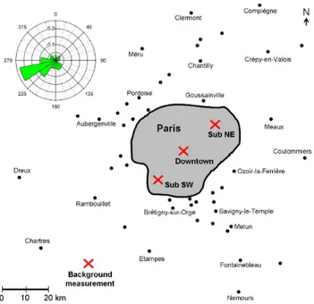
Measurement sites: three stationary measurement sites
were operated during the MEGAPOLI campaign (Fig. 1). The first one was located at the LHVP (Laboratoire d’Hygi`ene de la Ville de Paris) in the centre of the city (13th district, 2◦21033.7100E, 48◦49043.3600N) (further referred to as the “Downtown” site). The LHVP building faces to a smaller street in the north-west and to a park in the south-east, and is about 400 m south-east from Place d’Italie, where seven large Parisian avenues are intersecting. This site is con-sidered to represent Paris background air pollution (Sciare et al., 2010). The second station was located at a subur-ban site south-west from the city centre at SIRTA (Site In-strumental de Recherche par T´el´ed´etection Atmosph´erique, 2◦12026.3400E, 48◦4303.5900N, Haeffelin et al., 2005) (fur-ther referred to as the “Suburban SW” site, abbreviated “Sub SW”). This measurement site was located on the grounds of the Ecole Polytechnique and is surrounded by fields to the west and north-west, and by villages in 1–3 km dis-tance in the other directions. Major highways are located in about 3–6 km distance in all wind directions; a road with medium traffic is situated to the north in about 200 m dis-tance. The third station was set up at a suburban site in the north-east of the centre of Paris at the Golf D´epartemental de la Poudrerie (http://poudrerie.ucpa.com/, 2◦32049.1700E, 48◦5601.6700N, further referred to as the “Suburban NE” site, abbreviated “Sub NE”). This measurement site, located at the periphery of a residential area on a small employee parking lot, was bordered to the north (from east to west) by a golf course and a forested park; to the south there was a road with medium traffic density in about 30 m distance. The two latter sites are considered to be representative for suburban sites in-fluenced by local traffic emissions as well as the overall Paris emission plume. The three stationary sites were set up in a way that they provided connected flow conditions at SW and NE wind directions for quasi-Lagrangian measurements. The
Fig. 1. Location of the stationary measurement sites (Downtown,
Sub NE, Sub SW) and location of the short-time stationary back-ground measurement during the campaign using the Mobile Labo-ratory (see Sect. 3.4). The Paris agglomeration is indicated as grey area; cities outside this agglomeration are denoted as black dots for better orientation. In the upper left, the relative distribution of wind directions observed at Sub NE during the whole campaign is shown.
two suburban sites were located each in a distance of about 20 km from the Downtown site (see Fig. 1).
Sampling techniques: at each measurement site, a suite of
instruments was deployed for on- and off-line characteriza-tion of aerosol particle and gas phase as well as of meteorol-ogy. Here, only the sampling setups for the instruments used in the current analysis (Tables 1 and 2) are described.
At the Downtown site, gas analyzers as well as a TEOM-FDMS (tapered element oscillating microbalance – filter dy-namics measurement system) and a PILS-IC (particle-into-liquid sampler coupled to an ion chromatograph) were sam-pling on the flat roof top of the LHVP building at about 14 m height above ground level. Both aerosol instruments
were sampling through separate PM2.5 cyclones (model
SCC2.229, BGI Inc.). The PILS-IC was sampling through basic and acidic annular denuders (3-channel, URG Corp.), and daily filter measurements were performed to correct for background effects. The gas analyzers were located on the floor beneath the roof top and sampled via two independent
10 m long 1/400Teflon tubing sampling lines. A container was
located next to the LHVP building, about 25 m south-east of the roof top sampling inlets, adjacent to a small park. Here, sampling was conducted at about 6 m a.g.l., and the inlet was
equipped with a PM10 cyclone. This inlet was directly
fol-lowed by an automatic drying system (Tuch et al., 2009) to keep relative humidity (RH) below 30 % at all times. MAAP
Table 1. Instrumentation for measurement of the particle phase used in this study.
Parameter(s) Site Instrument Model (manufacturer) Time resolution Size range Uncertainty estimate for comparisonsa Particulate organics,
nitrate, sulphate, ammonium, chloride mass concentrations
Sub SW HR-ToF-AMS (Aerodyne Research, Inc.) 10 minb
∼PM1(lower size cut-off: ∼70 nm) 30 % PMF results: 20 % PMF mass concentrations: 36 %
Sub NE C-ToF-AMS 1 minc
Downtown HR-ToF-AMS 10 mind
MoLae HR-ToF-AMS 1 minf
Black carbon mass concentration
Sub SW Aethalometer Model AE31g(Magee Scientific) 2 min PM2.5 30 % Sub NE MAAP Model 5012 (Thermo Scientific) 1 min PM1 10 %
Downtown MAAP 1 min PM10
MoLa MAAP 1 min PM1
Particle number concentration
Sub NE CPC Model 5403 (Grimmh) 1 s >4.5 nm MoLa CPC Model 3786 (TSI Inc.) 1 s >2.5 nm
Particle number size distribution (dmob)
Sub SW SMPS Models 3080, 3081, and 3772i (TSI Inc.)
10 min 10.6–495.8 nm
Sub NE EAS (Airel Ltd.) 1 min 3.2 nm–10 µmj
MoLa FMPS Model 3091 (TSI Inc.) 1 s 5.6 nm–560 nm Particle number size
distribution (do)
Sub NE OPC Model 1.109 (Grimmh) 6 s 250 nm–32 µm
MoLa OPC 6 s
Particle number size distribution (dca)
Sub NE UV-APS Model 3314 (TSI Inc.) 5 min 500 nm–15 µmk
MoLa APS Model 3321 (TSI Inc.) 1 s 500 nm–20 µm Total aerosol mass
concentration
Sub NE TEOM-FDMS Models TEOM 1400a, FDMS 8500 (R&Pl)
15 min PM1
Downtown TEOM-FDMS 6 min PM2.5
Particulate sulphate mass concentration
Sub SW PILS-ICm 8 min PM2.5
Sub NE Quartz filters, off-line ICn
12 h PM1
Downtown PILS-ICm 15 min PM2.5
aSee main text for definition of uncertainty estimate used here.
bMeasurement cycle: 2.5 min each in V-mode ambient and thermodenuded, W-mode ambient and thermodenuded; MS/PToF cycles during V-mode: 10 s/10 s, W-mode:
only MS, 10 s cycles.
cMeasurement cycle: 20 s each in MS/PToF/LS mode.
dMeasurement cycle: 5 min each in V-mode and W-mode; MS/PToF-cycles W-mode: only MS in 40 s cycles; V-mode: MS/PToF in 20 s/40 s cycles. eMobile Laboratory.
fMeasurement cycle: V-mode, MS/PToF in 10 s/10 s cycles. g7-wavelength aethalometer.
hGrimm Aerosol Technik GmbH & Co. KG.
iClassifier model 3080, differential mobility analyzer model 3081, CPC model 3772. jOnly size range 4.86 - 486 nm used in the analysis (see text).
kOnly channels from 750 nm onwards used (see text). lRupprecht & Patashnick Co., Inc.
mPILS (Orsini et al., 2003) coupled to an ion chromatograph (Dionex, model ICS2000) equipped with a 2 mm diameter auto-suppression, anion self-regenerating
suppressor, a 2 mm diameter AS11-HC pre-column and column, and a 300 µL injection loop. For both PILS systems, liquid flowrates were delivered by peristaltic pumps set at 1.5 mL min−1for producing steam inside the PILS, and at Sub SW at 0.25 mL min−1for rinsing the impactor. At Downtown, a syringe pump was used at a flow of 0.8 mL min−1for rinsing the impactor, here two ion chromatography systems (for cation and anion quantification) and a TOC (total organic carbon) system were connected
to the PILS. For determination of anions, ion chromatography analysis was performed in isocratic mode at 12 mM of potassium hydroxide and a flowrate of 0.25 mL min−1.
n47 mm diameter pre-fired quartz filters (QMA, Whatman), analyzed using a 2 mm diameter AS11-HC model pre-column and column, a 20 µL injection loop, and an ion
chromatograph (IC, model DX-600, DIONEX) equipped with a reagent free system (automated eluent generation and self-regenerating suppression).
(multi-angle absorption photometer) and AMS (aerosol mass spectrometer) (amongst other instruments) were connected to this main inlet via 3/400and 3 m of 1/800stainless steel tub-ing, respectively. Particle losses for the AMS sampling line were estimated using the Particle Loss Calculator (von der Weiden et al., 2009), and were found to be below 10 % for the relevant size range (0.1–1 µm; mean value: ∼ 6 %).
At the Suburban SW site, several containers with measure-ment instrumeasure-ments were set up. AMS and SMPS (scanning mobility particle sizer), aethalometer and PILS-IC, and gas analyzers, respectively, were located in three separate con-tainers. For AMS and SMPS, sampling occurred at about 4 m
height a.g.l. through a PM10inlet. The aerosol was dried
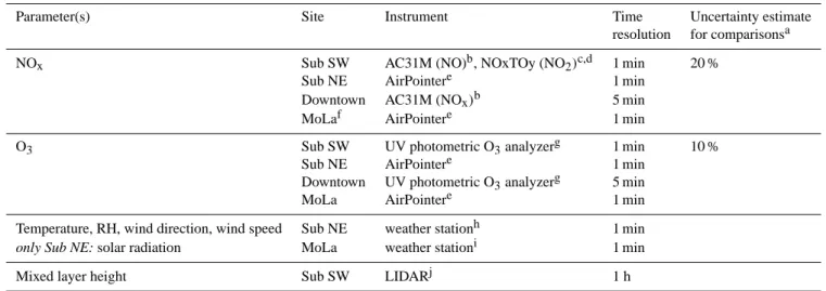
Table 2. Instrumentation for measurements of gas phase and meteorological parameters used for this analysis.
Parameter(s) Site Instrument Time Uncertainty estimate resolution for comparisonsa NOx Sub SW AC31M (NO)b, NOxTOy (NO2)c,d 1 min 20 %
Sub NE AirPointere 1 min Downtown AC31M (NOx)b 5 min
MoLaf AirPointere 1 min
O3 Sub SW UV photometric O3analyzerg 1 min 10 %
Sub NE AirPointere 1 min Downtown UV photometric O3analyzerg 5 min
MoLa AirPointere 1 min Temperature, RH, wind direction, wind speed Sub NE weather stationh 1 min
only Sub NE: solar radiation MoLa weather stationi 1 min
Mixed layer height Sub SW LIDARj 1 h
aSee main text for definition of uncertainty estimate used here.
bAC31M, Environnement S.A. (detection of NO using ozone chemiluminescence; detection of NO
xusing ozone chemiluminescence after thermal conversion to NO on
molybdenum-converter).
cNOxTOy, METAIR (detection of NO
2using chemiluminescence of luminol). dNO
xwas calculated from (NO+NO2).
eAirPointer, recordum Messtechnik GmbH (UV photometric detection of O
3; detection of NOxas underb).
fMobile Laboratory.
gModel 49C, Thermo Environmental Instruments. hVantage Pro2, Davis Instruments.
iVaisala.
jWind Lidar Leosphere; mixed layer height retrieved using STRAT-2D algorithm (see text).
tubing to the instruments. The inlets for aethalometer and
PILS-IC, located at 4 m a.g.l., were equipped with PM2.5
cy-clones (R&P and BGI Inc., respectively). The denuder sys-tem and the filter measurements for the PILS-IC were equal to those at the Downtown site. Gas analyzers were sampling via Teflon tubing from about 3.5 m height a.g.l.
At the Suburban NE site, all instruments were located in one container with an inlet at about 8 m above ground. The EAS (electrical aerosol spectrometer) was sampling directly from the main inlet. Insulated 1/200stainless steel tubing con-nected OPC (optical particle counter), UV-APS (ultraviolet aerodynamic particle sizer), MAAP, TEOM-FDMS, and
fil-ter sampler to the main inlet; 1/400 tubing was used to
con-nect the AMS and CPC (condensation particle counter). PM1
cyclones were located directly in front of the MAAP, the TEOM-FDMS, and the filter sampler inlets, respectively. The aerosol sampled by OPC and UV-APS was dried using a sil-ica gel diffusion drier. The sampling losses for this whole inlet system were calculated using the Particle Loss Calcu-lator (von der Weiden et al., 2009), and were for all instru-ments below 10 % in their relevant measurement size range, with largest losses for smallest and largest particle sizes. In-let losses for UV-APS and OPC for particle diameters larger than 5 µm were higher (approximately 30 % at 10 µm
diam-eter). The weather station and the inlet to the 1/400 Teflon
sampling line for the gas analyzers were also located at the main inlet at about the same height as the aerosol inlet.
At the Suburban NE site, also the Mobile Laboratory MoLa (Drewnick et al., 2012) was stationed when not op-erating in the field, and measuring side by side to the sta-tionary laboratory at about the same inlet height. The Mo-bile Laboratory was also measuring for one day each at both the Sub SW and the Downtown sites, respectively, for inter-comparison purposes (Sect. 2.2). Furthermore, in Sect. 3.4 one selected stationary measurement of the Mobile Labora-tory outside of Paris is used to complete the data base for the analysis.
2.2 Data acquisition and validation
The data acquisition of all instruments is described in Sect. 2.2.1, except for the AMS, which is treated in Sect. 2.2.2. As already mentioned, measurement data from the intercomparison periods (Sub NE: 274 h distributed over the whole campaign; Downtown: 17 July, 10:20–18:30; Sub SW: 23 July, 11:20–19:00) were used to compare the various instruments at the different sites to the instruments on-board the Mobile Laboratory. From these comparisons, estimates for the comparability of measurements from different sites have been deduced (see Tables 1 and 2). Note that these es-timates do not reflect the uncertainty of the instruments or the measurements itself, but are solely used as a mean to en-sure the comparability of meaen-surements between the differ-ent sites. This also includes variations due to differdiffer-ent sam-pling or working principles of the instruments. The results
of these intercomparisons are discussed in the following two sections.
2.2.1 Comparability of non-aerosol mass spectrometer measurements
Details on the instruments used (model and manufacturer) as well as on sampling intervals can be found in Tables 1 and 2, along with the estimated uncertainties of the associated measurements for comparison purposes. All intercomparison results are given in the Supplement in Tables S1 and S2 in detail. The main results are briefly summarized here.
Black carbon (BC) measurements from MAAPs at Sub NE, Downtown and the Mobile Laboratory showed good agreement (within 10 %). Differences in cut-offs did not seem to have a significant influence, confirming that BC is predominantly found in the submicron range (Seinfeld and Pandis, 2006). The aethalometer at Sub SW measured higher concentrations during the intercomparison period, compared to the MAAP on-board the Mobile Laboratory. We attribute this to instrumental differences which might limit the com-parability with the MAAP measurements. Therefore, for the aethalometer, a larger uncertainty of 30 % is assumed here for comparison purposes.
Ozone (O3)did show very good agreement in all
inter-comparisons (uncertainty estimated to 10 %). NOxwas
mea-sured using different techniques at the various sites (see Ta-ble 2). Despite this fact, at all sites the intercomparison mea-surements showed good agreement within an uncertainty of 20 %.
The OPC and CPC at Sub NE showed good agreement with the OPC and CPC on-board the Mobile Laboratory, re-spectively (within 10 and 30 %, rere-spectively; the larger devi-ation for the CPC measurement is explainable by the differ-ences in lower cut-offs of the instruments, see Table S2 for details). The UV-APS was only comparable (within 20 %) to the Mobile Laboratory APS for particles with
continuum-aerodynamic diameter dca≥750 nm, likely due to slight
in-strumental differences. Therefore, only data for particle sizes from 750 nm onwards are used for the analysis. The size ranges of the EAS at Sub NE and the FMPS (fast mobility particle sizer) on-board the Mobile Laboratory overlap only
between 4.86 and 486 nm (mobility diameter, dmob).
There-fore, comparison between the two instruments is only possi-ble in this size range, and consequently only this size range has been used in the analysis. The comparison shows a mode in the number distribution measured by the FMPS around 10 to 15 nm which is likely an artefact due to the inversion algorithm used for this instrument (A. Wiedensohler, per-sonal communication, 2012). The EAS does not show this mode, possibly due to differences in the analysis software used. However, no direct intercomparison measurements to SMPS systems were available for the EAS. Therefore, es-pecially the smaller size mode (up to about 20 nm) has to be regarded with a higher uncertainty than the coarser size
mode above 20 nm. For these larger particle sizes, the com-parisons between FMPS and SMPS systems showed good agreement, and also the EAS and FMPS agree reasonably well (FMPS versus EAS number size distribution for sizes
above 20 nm: slope m = 0.80, Pearson’s R2=0.84; total
particle number concentrations agree within 15 % for parti-cle sizes above 20 nm, else within 30 %). 12 h filter samples were taken on 47 mm quartz filters from which particulate sulphate was quantified using ion chromatography (IC); they were corrected from routinely taken blank filters. Meteoro-logical data showed excellent agreement between the Mobile Laboratory and Sub NE. Furthermore, a comparison to wind data routinely measured at Sub SW showed little difference in the local wind speed and direction measured at the dif-ferent sampling sites. Therefore, for the analysis, only me-teorological data measured at Sub NE are used. The mixed layer height has been determined at Sub SW from routinely measured LIDAR (light detection and ranging) data using the STRAT-2D algorithm described in Haeffelin et al. (2012).
2.2.2 Aerodyne aerosol mass spectrometer measurements
At Sub NE, a C-ToF-AMS (compact time-of-flight aerosol mass spectrometer; Drewnick et al., 2005) was used, while at the other sites including the Mobile Laboratory, a HR-ToF-AMS (high-resolution HR-ToF-AMS; DeCarlo et al., 2006) was deployed. These instruments were used to measure the submicron mass concentrations and size distributions of non-refractory particulate organic matter (“organics”), sulphate
(“SO4”), nitrate (“NO3”), ammonium (“NH4”), and chloride
(“Chl”). All instruments measured at about 600◦C vaporizer
temperature, only the Sub NE AMS was measuring at about
800◦C during the first two weeks of the campaign (30 June–
14 July) to gather information concerning the dependency of organic fragmentation patterns on vaporizer temperature. However, no significant differences in organic fragmentation patterns or in mass concentrations due to heater temperature differences could be found in the semi-continuous intercom-parison with the Mobile Laboratory AMS. Information on AMS measurement cycles can be found in Table 1. For the Downtown and the Sub SW site, we present only ambient MS (mass spectrum mode, yielding the average mass con-centrations as described above) data acquired in V-mode, the lower resolution mode of the HR-ToF-AMS (as opposed to the higher resolution in W-mode). For the Sub NE site, only MS and PToF (particle time-of-flight mode, yielding the av-erage mass size distributions) data are used. The C-ToF-AMS at the Sub NE site was additionally equipped with a light scattering probe (Cross et al., 2007), enabling single particle analysis. Results from this will be presented in an upcoming publication.
For all instruments, weekly calibration measurements of
NH4NO3 particles (measurement in brute force single
and Downtown, 350 nm at Sub NE, and 550 nm in the Mo-bile Laboratory) to determine the AMS ionisation efficiency (IE), and measurements of filtered, particulate-free ambi-ent air to correct for background effects have been per-formed throughout the campaign. A collection efficiency (CE) of 0.5 was assumed for all instruments as a typi-cal value for fully neutralized, internally mixed particles with low to moderate nitrate content (Matthew et al., 2008). This CE was validated by comparisons with other instru-ments as described below. Standard relative ionisation
ef-ficiency (RIE) values (for SO4: 1.2; organics: 1.4; NO3:
1.1; NH4: 4) were used if not noted otherwise below.
The data analysis was performed with SQUIRREL (ver-sions 1.48 to 1.51C, http://cires.colorado.edu/jimenez-group/ ToFAMSResources/ToFSoftware/), applying the standard fragmentation table (Allan et al., 2004, with modifications according to Aiken et al., 2008, except for the Downtown site) with the respective individual corrections inferred from the measurements of particulate-free air.
Data validation for the different instruments: during
the stationary measurements, the Mobile Laboratory AMS showed neutralized to slightly acidic aerosol within its mea-surement uncertainties. For 15 min averaged data, the lin-ear fit through zero yielded a slope (m) of 1.32 and Plin-ear- Pear-son’s R2of 0.97 for the correlation of measured (NOmolar3 +2 SOmolar4 +Chlmolar)versus NHmolar4 , with Xmolarmeaning the
molar concentration of species X (Fig. S1a). For NH4, a RIE
of 4.1 was used, which was inferred from the NH4NO3
cal-ibrations performed in MS mode. The total submicron par-ticulate mass concentration measured by the Mobile Labora-tory AMS plus the BC concentration measured by the MAAP on-board the Mobile Laboratory when parked at the Sub NE
site agreed reasonably well with the total PM1 mass
con-centration measured by the TEOM-FDMS at the same site
(m = 0.90, R2=0.45). Therefore, the AMS on board of the
Mobile Laboratory seems well suited as reference instrument for the other AMSs.
For the AMS at Sub NE, laboratory calibration
measure-ments of (NH4)2SO4 were performed to determine the RIE
of SO4. This gave an RIE of 0.76. From the ammonium
ni-trate calibration measurements (MS mode) during the
cam-paign, a RIE of 4.2 was estimated for NH4. Using those
RIE values, comparison of AMS SO4 to filter
measure-ments of particulate sulphate (using IC) showed satisfying
agreement (m = 1.18, R2=0.72), and the aerosol was found
to be neutralized to slightly acidic (m = 1.05; R2=0.99)
(Fig. S1b). However, comparison to the Mobile Laboratory AMS showed significantly smaller organic mass concentra-tions for this instrument (Table S3). Direct comparison of the mass spectra of both instruments showed that this was likely due to the smaller ion transmission in the Sub NE AMS at larger mass to charge ratios (m/z’s) compared to the Mobile Laboratory AMS, which is also the reason for
the smaller RIE of SO4 than typically used. Therefore,
or-ganics measured by the AMS at Sub NE were scaled with a factor of 1.5 (which would correspond to an effective RIE of organics of 0.93) to account for this effect. After this scaling, comparison of total mass concentration measured
by MAAP and AMS with the total PM1 mass
concentra-tion measured by TEOM-FDMS showed good agreement
(m = 0.94, R2=0.74) (Fig. S2).
At the Downtown site, due to a power failure during the night before the intercomparison measurement, the AMS was completely turned off, and only restarted directly be-fore the intercomparison period (which therebe-fore lasted only for ∼ 5 h). Also, AMS measurements of particulate-free air could only be performed after the intercomparison, when the background already had decreased. Therefore, background values for the intercomparison period itself cannot be
ac-counted for correctly. This affects especially NH4, for which
a large discrepancy in measured mass concentrations be-tween the two instruments was found, while all other species agree within ∼ 10 % (Table S3). The measured aerosol was neutralized to slightly acidic at this site throughout the
campaign (m = 1.18, R2=0.99) (Fig. S1c). Comparison of
AMS SO4 with sulphate mass concentrations from
PILS-IC PM2.5 measurements (m = 0.95, R2=0.76) and of
to-tal particle mass concentrations from AMS and MAAP to
TEOM-FDMS PM2.5(m = 0.87, R2=0.46) showed
reason-able agreement, especially when considering the different upper size cut-offs of the instruments.
For the AMS at the Sub SW site, a RIE for NH4of 3.3 was
determined from the NH4NO3 measurements in MS mode.
Still, comparison to the Mobile Laboratory AMS shows large
discrepancies around 30 % for all species except for NH4,
for which the discrepancy is even larger (∼ 70 %) (Table S3). These large and systematic negative differences of all species are likely due to large sampling losses, or to systematic errors in the IE calibration. Therefore, in order to be able to com-pare the measurements from the instruments of all sites, a general scaling of the Sub SW AMS to the Mobile Labora-tory AMS measurements using a scaling factor of 1.3 for all species (see Table S3) was applied. After this scaling,
com-parison of SO4measured with the Sub SW AMS to sulphate
from PILS-IC PM2.5 measurements at the same site gives a
more reasonable result (m = 0.87, R2=0.92; before
scal-ing: m = 0.67), despite differences in cut-offs. The aerosol measured with the Sub SW AMS was found to be neutral-ized to slightly acidic within the uncertainties throughout the
whole campaign (m = 1.29, R2=0.99) (Fig. S1d).
How-ever, no total aerosol mass concentration measurement was performed at this site, so only comparisons to total particle mass concentrations calculated from SMPS measurements are available. To convert mass concentrations into total par-ticle volume concentrations, parpar-ticles were assumed to be spherical and to exhibit a time-dependent density. The lat-ter was inferred from the varying chemical composition and from densities of 1.72 g cm−3for NH4NO3, 1.77 g cm−3for
(the average density of the whole campaign would
corre-spond to 1.65 g cm−3). The sum of calculated total particle
volume from BC mass concentration and total mass concen-trations measured with the AMS agrees reasonably well with the SMPS total particle volume concentration (m = 0.93,
R2=0.54; before scaling: m = 0.74, R2=0.56) (Fig. S3).
The upper size cut-off of the SMPS at about 500 nm (dmob)
corresponds to a vacuum-aerodynamic diameter of about 800 nm, which is similar to the cut-off for the BC and AMS measurements. All in all, these comparisons seem to validate the scaling procedure for the Sub SW AMS.
For all validated AMS measurements, a total uncertainty of 30 % is assumed, including uncertainties from RIE, IE, and CE determination. This is in line with typically observed uncertainties from instrumental comparisons of the AMS (Canagaratna et al., 2007).
2.3 Positive matrix factorization of AMS measurements
Positive matrix factorization (PMF; Paatero and Tapper, 1994) was applied to the time series of mass spectra of organ-ics measured with the AMSs. PMF mathematically retrieves a given number of constant factor profiles (mass spectra in the case of AMS) and their contribution to the total measured mass spectrum for each time step by minimizing the residual between measured and modelled data, achieving both time series and mass spectra of a given number of factors with-out a priori information. To explore the possibility of dif-ferent local minima, usually PMF solutions from a number of different randomly chosen starting points (“seeds”) are explored. Furthermore, the factor solutions derived by PMF are not unique, but (approximate) rotations of the matrices of factor time series and mass spectra may result in solutions which still meet the convergence criteria. This rotational am-biguity is explored by varying the so-called “fpeak” parame-ter. Details on application of PMF to AMS data can be found in (Ulbrich et al., 2009). The PMF Evaluation Tool (PET, version 2.03A) described by Ulbrich et al. (2009) was used in this analysis using the PMF2 algorithm (Paatero, 1997). For the three AMS datasets, matrices with the time series of the organics mass spectra and the associated errors were re-trieved from SQUIRREL using the standard fragmentation table (Allan et al., 2004). Details on the data matrix treat-ment for preparation for PMF and on the PMF analysis itself can be found in Table S4. From all datasets, individual ex-traordinarily high data points (“spikes”) in the data and error matrices, which could not be fitted appropriately by the al-gorithm, were removed iteratively. From the Sub NE dataset, furthermore two time periods of a few hours each were re-moved which were measured during nearby fireworks on the night before 14 July, and during residential trash burning in the neighbourhood on 11 July to avoid artificial biases of the PMF analysis. For further validation of the method, for the Sub NE dataset, PMF was performed both on the whole dataset and for the periods with higher and lower heater
tem-perature separately, however, no significant differences were found. Therefore, only the PMF solutions using the whole dataset were evaluated further and are presented here. For all datasets, the pre-defined number of factors to be calculated by PMF was varied from 1 to 5 with a “coarse” variation of
fpeak parameters (see Table S4). The two-factor solution was
found to explain best the data from the Sub NE and the Sub SW site, while for the Downtown site, both the two- as well as the three-factor solution were found suitable. These results are discussed in more detail in Sect. 3.1. For the Sub SW and Downtown site, the solutions with more factors showed split-ting of the factors, which after inspection of mass spectra and time series were identified as physically meaningless. For the Sub NE site, the third factor obtained in the three-factor so-lution was driven by instrumental noise and could not be suppressed by any data pre-treatment. This factor was still present also at higher factor solutions (solutions with more factors). Furthermore, these higher factor solutions resulted again in a physically meaningless splitting of the other fac-tors. Therefore, only the two-factor solution was used for fur-ther analysis. In all cases, also fpeak and seed variations did not provide more reasonable results for higher factor solu-tions. Time series and mass spectra of higher factor solutions for the different sites are shown in the Supplement (Figs. S4 to S6).
For the chosen number of factors, fpeaks were varied in steps of 0.1 from −1.5 to 1.5. There was no indication that any other solution than those with fpeak = 0 might provide physically more meaningful results. Therefore, fpeak = 0 was used for the further analysis. In addition, seeds were varied from 0 to 50 in steps of 1 for the chosen solutions at fpeak = 0. No differences in the solutions at varying seeds were found for the chosen solutions with exception of the three-factor solution at the Downtown site, where 2 out of 51 solutions gave slightly different results, but with very sim-ilar time series and mass spectra as for the other solutions. Therefore, only the seed = 0 solutions were regarded further. However, the variation of the results upon varying fpeaks and
seeds were used as a measure of the uncertainty of the
cho-sen PMF solutions, both for the obtained factor mass spec-tra and the time series. To calculate these uncertainties, for each data point (m/z or time step, respectively) the average and the standard deviation of all solutions was calculated. To calculate the relative uncertainty of the mass spectra (1MS),
the sum of the absolute standard deviations for the individual
m/z’s was calculated and divided by the sum of the signal
of the average mass spectrum (Eq. 1). For calculation of the relative uncertainty of the factor time series (1TS)according
to Eq. (2), the time series of the absolute standard deviations was divided by the average time series to give the relative standard deviation of each data point. The average of these relative standard deviations gave the overall uncertainty of the time series.
1MS= n P i=1 σp,i n P i=1 ¯ xp,i (1) 1TS= n P i=1 σp,i ¯ xp,i n (2)
n: the number of m/z’s or time steps, respectively; ¯xp,i: the
average for one m/z or time step; σp,i: the standard deviation
for one m/z or time step.
The calculated uncertainties for all PMF results can be found in Table S5. In general, the uncertainties from seed variations are much smaller than those from fpeak varia-tions (e.g., for the two-factor soluvaria-tions, uncertainties from
seed variations are around 1 %, while fpeak variation
usu-ally gives uncertainties of the order of 10–20 %), indicat-ing that the solutions are relatively stable independent of the chosen seed. Relative uncertainties of time series are usually slightly larger than those of the mass spectra, but of the same order of magnitude. All estimated uncertainties (from fpeak and seed) for the two-factor solutions from the different sites are below about 20 %. The uncertainties for the Downtown three-factor solution are larger, especially for the two differ-ent HOA (hydrocarbon-like organic aerosol) factors (up to about 40 %). This reflects the associated uncertainty in the retrieval of factors related to different sources (and therefore, with different time series), but with very similar mass spec-tra.
As discussed in Sect. 3.1, only the two-factor solutions from all sites are used for the following study. From the es-timated uncertainties given in Table S5, an upper limit of uncertainty at about 20 % for these two-factor solutions can be deduced. This uncertainty of the PMF analysis, together with the uncertainty of the AMS measurement itself (30 %), results in a total uncertainty for the absolute mass concentra-tions of the individual organic aerosol types from the PMF solutions of ((30 %)2+(20 %)2)1/2=36 %.
PMF solutions of the AMS measurements in the Mobile Laboratory as described in von der Weiden-Reinm¨uller et al. (2013) are also used in the following analysis. Those re-sults are described in Sect. 3.1.
2.4 Particle dispersion model FLEXPART
The Lagrangian particle dispersion model FLEXPART (Stohl et al., 2005), version 8.2, was used to assess the ori-gin of air masses sampled at the stationary sites. 20-day backward simulations were performed for the Sub NE site at 3 h time resolution using ECMWF (European Centre for Medium-Range Weather Forecasts) meteorological data by releasing 60 000 particles at the measurement location and
following them backward in time. In this analysis, for the de-termination of air mass origin, footprint emission sensitivities for aerosol tracers were used. The so-called emission
sensi-tivity is proportional to the residence time of the particles
over a given grid cell, while the footprint emission sensitivity represents this emission sensitivity integrated over the low-est 100 m of the atmosphere. The footprint emission
sensitiv-ity therefore gives an indication where emissions could have
been taken up effectively by the air mass that arrived at a cer-tain time at the measurement site. Multiplying the footprint
emission sensitivity with emission fluxes from a spatially
dis-aggregated inventory gives the distribution of emissions con-tributing to the simulated mixing ratio at the receptor site. Removal processes for aerosol particles (wet and dry deposi-tion) are also taken into account in the simulations.
Furthermore, for each 3 h data point, the integral of
foot-print emission sensitivity over the total land surface area has
been calculated. This integral gives the absolute continental contribution to the footprint emission sensitivity for a given air mass, and therefore gives an indication for the amount of continental influence on the sampled air masses.
3 Results and discussion
3.1 Identification of the PMF factors
Correlations of the time series of the PMF factors found for the different sites (as described in Sect. 2.3) with time se-ries of external tracers, measured at the respective site (SO4,
NO3 from AMS measurements, and BC and NOx)are
pre-sented in Table S6. Correlations of the factor mass spectra with reference mass spectra from the literature are shown in Table S7.
For the two-factor solutions, time series of factor 1 of the three sampling sites correlate better with time series of
pri-mary emission tracers (NOxand BC, Pearson’s R2usually
on the order of 0.2 to 0.3) than with that of secondary species
(SO4and NO3, R2usually below 0.1). The respective mass
spectra correlate very well (Pearson’s R2typically about 0.8)
with reference mass spectra of HOA (hydrocarbon-like ganic aerosol; Ulbrich et al., 2009) and cooking-related or-ganic aerosol (Allan et al., 2010; He et al., 2010), which both are related to primary emissions. Time series of fac-tor 2 of all three sampling sites correlate with time series of
secondary species (SO4 and NO3, R2 typically around 0.5
and 0.2–0.3, respectively), and the respective mass spectra correlate very well with low-volatile OOA (low-volatile
oxy-genated organic aerosol, R2about 0.9) and to a lesser extent
also with semi-volatile OOA (semi-volatile oxygenated
or-ganic aerosol, R2about 0.6 to 0.7) (both from Ulbrich et al.,
2009). Therefore, we classify factor 1 of all three sampling sites as comparably fresh “HOA”, while factor 2 is identified as more aged “OOA”. These classifications are summarized in Table S6.
The correlations of the OOA factor time series are
gener-ally better with SO4mass concentration time series than with
those of the semi-volatile NO3. Furthermore, the retrieved
factor mass spectra do resemble more low-volatile OOA than semi-volatile OOA reference mass spectra (Table S7). Both observations point to the fact that the retrieved OOA factors are dominated by low-volatile rather than semi-volatile or-ganic compounds. Semi-volatile OOA is thought of as hav-ing an oxidation state between HOA and low-volatile OOA (Jimenez et al., 2009); therefore it is not surprising that mass spectra of the retrieved HOA and OOA classes do correlate with the reference mass spectrum of semi-volatile OOA sim-ilarly (R2about 0.5 to 0.7), but neither exceptionally well.
The correlations of the HOA factor time series with the primary emission tracer time series are better than those with
secondary species, but still rather low (R2usually about 0.2
to 0.3). For the Downtown site, the HOA factor can be split up into two HOA-like factors when moving from the two- to a three-factor solution (Fig. S5). From these factors, one fac-tor (facfac-tor 3) correlates much better with the primary
emis-sion tracer time series (R2about 0.5 to 0.7), while the other
(factor 1) correlates much worse (R2<0.2). In addition, fac-tor 3 shows a much better similarity with HOA reference mass spectra than the HOA from the two-factor solution. Since HOA usually is associated with emissions from traf-fic (e.g., Zhang et al., 2011), as are also the primary emission
tracers NOxand BC, this all together indicates that factor 3
represents a part of the total HOA from the two-factor solu-tion which is likely traffic-related.
Figure 2 shows the diurnal cycles of all HOA-like fac-tors retrieved for the Downtown site with the different PMF solutions. The more traffic-related HOA-like factor (HOAtraffic rel.)from the three-factor solution peaks during
the morning and the evening hours, consistent with rush hour times. The other HOA-like factor from the three-factor solu-tion shows a peak during the evening and around noon, when
no peaks in NOxand BC are observed (Fig. 5a). Such a
di-urnal pattern for a HOA-like PMF factor was also observed e.g. by Allan et al. (2010) in Manchester and London and at-tributed to cooking-related primary emissions. Similar to our findings, also Allan et al. (2010) found only a weak corre-lation of the time series of this factor with that of BC. The interpretation of this factor (factor 1 of the three-factor
solu-tion) as “cooking-related organic aerosol” (HOAcooking rel.)
would be reasonable since the Downtown measurement site was situated in an area where several restaurants are located. However, comparison with reference mass spectra proves difficult, as the mass spectra found for traffic- and cooking-related emission sources are very similar. Both the mass spectra of our more traffic-related HOA factor as well as the apparently more cooking-related HOA factor correlate well (R2>0.8) with the cooking-related organic aerosol fac-tors found by Allan et al. (2010); however, contrary to
ex-pectations, our HOAcooking rel.factor correlates worse (R2=
0.64) with cooking-related organic aerosol source spectra
Fig. 2. Diurnal pattern (hourly median values for the whole
cam-paign) of HOA from the two-factor solution, and the two HOA-like factors (HOAtraffic rel., HOAcooking rel.)from the three-factor
solu-tion retrieved for the Downtown site. Percentiles (25 and 75 %, light grey shading) are only shown for HOA from the two-factor solution for clarity.
published by He et al. (2010) than the HOAtraffic rel.
fac-tor (R2=0.80). Thus, further work is needed to
character-ize varying cooking sources and get a more comprehensive dataset of mass spectra and typical mass spectral markers characteristic for ambient, cooking-related organic aerosol. The diurnal pattern of the HOA especially from the Sub NE site is similar to that of the Downtown site two-factor so-lution HOA (Fig. S7). Therefore, it cannot be excluded that also the HOA factors of the suburban sites contain a con-tribution from cooking-related organic aerosol. This would also explain the low correlations of the HOA factors with
NOx and BC for these two sites. However, due to the mass
spectral similarity of HOAtraffic rel. and HOAcooking rel., this
separation of the two HOA factors cannot be achieved for the Sub SW and Sub NE site, which are not located in a region with as many cooking-related sources nearby as the Down-town site.
For Sub SW, the two aforementioned HOA factors can be distinguished via PMF of the high resolution mass spectra (Crippa et al., 2013b). However, within the framework of this paper, where we compare measurements at the three differ-ent stationary sites, only the two-factor solutions from PMF of unit mass resolution mass spectra are used for all sites for better comparability. As both, traffic- as well as cooking-related emissions, are generated by local primary emissions opposed to more aged secondary species within the OOA fac-tor, and since this is the main information needed for the fol-lowing analysis, this mixture of different sources within a single factor is no drawback.
For the Mobile Laboratory AMS measurements during this campaign, von der Weiden-Reinm¨uller et al. (2013) were able to identify a physically meaningful four- and a five-factor solution from the PMF analysis. In the four-five-factor so-lution, one traffic-related HOA-like factor (HOAtraffic rel.),
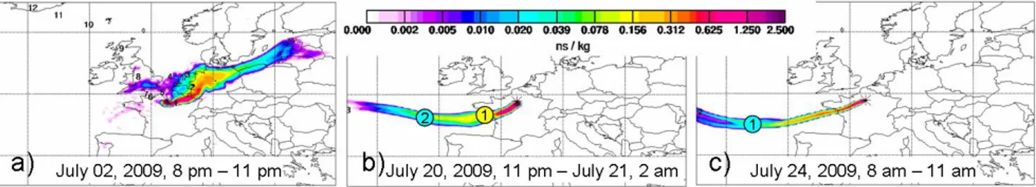
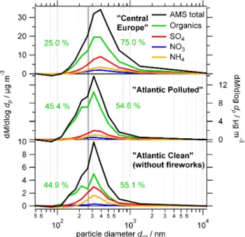
Fig. 3. Examples for (a) “Central Europe”, (b) “Atlantic Polluted”, and (c) “Atlantic Clean” air masses distinguished using FLEXPART
footprint emission sensitivities. The numbers in circles denote the approximate location of the centroid of the air mass at the respective
number of days prior to sampling.
semi-volatile like factor, and one low-volatile OOA-like factor were retrieved. The first three factors were found to be associated with the Paris emission plume. In the five factor solution, one more semi-volatile OOA-like factor was retrieved, which originates from both the low-volatile OOA-like and the three plume-related factors from the four-factor solution. For the four-factor solution, from the long-term intercomparison measurements at the Sub NE site, it was found that low-volatile OOA retrieved from the Mobile Lab-oratory AMS data corresponds to the OOA retrieved from
the Sub NE site data (Pearson’s R2 for linear correlation
of time series: 0.91; for mass spectra: 0.99), while the sum of HOAtraffic rel., HOAcooking rel.and the semi-volatile
OOA-like factors of the Mobile Laboratory AMS (this sum further referred to as “HOA” for the Mobile Laboratory) corresponds
to the HOA retrieved at the Sub NE site (R2for time series:
0.81; for mass spectra: 0.90). From the intercomparison mea-surements at all stationary sites, good correlations between the OOA and the HOA factor time series of the Mobile Lab-oratory and the respective sites are found (Table S8), with a deviation within the uncertainty of 20 % which was calcu-lated for the PMF factors in Sect. 2.3. Also the mass spectra (Fig. S8) exhibit the same features for each organic aerosol type at all sites. For the five-factor solution, the “new” semi-volatile OOA cannot be assigned clearly to either the OOA or the HOA from the stationary sites. Therefore, in the fol-lowing analysis, HOA and OOA from the two-factor solu-tions for the stationary sites, and the corresponding OOA and combined HOA-like factors from the four-factor PMF solution for the Mobile Laboratory (combined as described above) are compared to each other within the associated un-certainty discussed in Sect. 2.3.
3.2 Classification of air masses
The air masses sampled at the stationary sites were classified using the output of the FLEXPART simulations described in Sect. 2.4. Three major classes of air masses were distin-guished: “Central Europe”, “Atlantic Clean”, and “Atlantic Polluted”.
Only during the first days of the field campaign, air masses from eastern continental Europe were advected; an exam-ple is shown in Fig. 3a. These air masses, which had trav-elled for several days over polluted continental regions, were classified as “Central Europe” air masses. For the remaining time of the campaign, air masses were mostly advected from south-westerly to north-westerly directions, namely from the Atlantic Ocean, passing western France on different routes. They were classified as “Atlantic Clean” or “Atlantic Pol-luted” air masses, depending on their residence time over continental areas. This residence time was estimated using the location of the centroid of the air mass 24 h prior to sam-pling (provided from the FLEXPART simulations, denoted with a circled “1” in Fig. 3b and c). Air masses which were travelling rather fast (which means, the centroid of the air mass was far outside the French west coast one day prior to sampling; this corresponds to a travelling velocity of the air mass of approximately 1200 km per day, i.e. an average
transport velocity of ∼ 14 m s−1)were regarded as “Atlantic
Clean”, as they did not have a long residence time over con-tinental areas (Fig. 3c) before arriving at the Paris metropoli-tan area. Air masses at the coast or over land one day prior to sampling were classified as “Atlantic Polluted” (Fig. 3b), un-less removal processes especially via precipitation had taken place during the last two days of the travelling time of the air mass before arrival at the sampling sites, in which case they were classified as “Atlantic Clean”. Furthermore classified as “Atlantic Polluted” were air masses which had remained for a longer period of time over Spain and the heavily anthro-pogenically influenced region in the Atlantic Ocean between Spain and France.
The resulting time series of various aerosol components, measured with the AMSs at the three stationary sites, to-gether with the air mass classification are shown in Fig. 4. The uppermost panel of Fig. 4 shows the time series of the absolute continental contribution to the footprint
emis-sion sensitivity of the sampled air masses as calculated from
FLEXPART (see Sect. 2.4). In total, 62 h of “Central Eu-rope”, 257 h of “Atlantic Polluted”, and 423 h of “At-lantic Clean” air masses were sampled during the whole
Fig. 4. Classification of the sampled air masses (orange, green, and
blue background for “Central Europe”, “Atlantic Polluted”, and “At-lantic Clean” air masses, respectively), time series of calculated ab-solute continental contribution to footprint emission sensitivity, and selected species (SO4, NO3, NH4, organics, and OOA and HOA retrieved from total organics using PMF) measured with the AMS at the three stationary sites (Sub NE: medium coloured, Downtown: light coloured, Sub SW: dark coloured curves). Some local events at single sites in the time series of NO3and SO4 as discussed in
Sect. 3.3.1 are marked.
measurement period. A discussion of the characteristics of the different types of air masses is given in the next section.
3.3 Influence of air mass origin and meteorology 3.3.1 Averages and diurnal cycles
Averages of selected meteorological, gas phase and particle phase parameters for the different sites and air masses are given in Table 3. The origin of air mass was similar for both “Atlantic” air masses, which is also reflected in the average wind directions (south to south-west for the “Atlantic” air masses, north-east for “Central Europe” air masses). On the other hand, meteorological parameters such as average tem-perature and wind speed were more similar between “Cen-tral Europe” and “Atlantic Polluted” air masses.
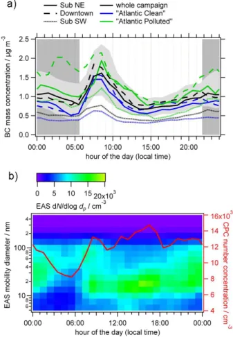
Tempera-Fig. 5. (a) Diurnal cycles (hourly median values) of BC mass
con-centration at the three stationary sites (for the whole campaign, and for “Atlantic Polluted” and “Atlantic Clean” air masses separately). Percentiles (25 and 75 %) are shown exemplarily in light grey for the measurement at Sub NE (whole campaign); all other percentiles are omitted for clarity. The time period between sunset and sunrise is shaded in grey. (b) Diurnal cycles (hourly median values) of EAS number size distribution and CPC number concentration measured at the Sub NE site.
ture was lower and wind speed was higher on average for the “Atlantic Clean” air masses. Since, by definition, the rel-evant difference of the “Atlantic Clean” air masses from the “Atlantic Polluted” air masses is the shorter residence time over land, this higher average wind speed associated with the former air masses is not surprising. The differences in resi-dence time over land for all three air mass categories are also evident in the continental contribution to the footprint
emis-sion sensitivity, which from the FLEXPART calculations was
found to be highest for “Central Europe” air masses, and low-est for the “Atlantic Clean” air masses.
Primary emission tracers: at all sites, the diurnal cycles
of the primary emission tracers BC (Fig. 5a), HOA (Figs. 2
and S7), and NOx(not shown; the diurnal cycle is
compara-ble to that of BC) show peaks during the morning and the evening rush hours, consistent with their association with
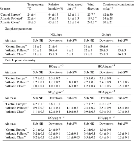
Table 3. Meteorological parameters measured at and modelled for Sub NE; gas phase parameters and particle chemical composition measured
at the respective sites. Given are the averages with uncertainty ranges as deduced in Sect. 2, except for meteorological parameters, where means and standard deviations are provided. Chloride as measured by the AMS was below 0.1 µg m−3at all sites for all averages and was therefore not regarded for this analysis.
Meteorology
Temperature/ Relative Wind speed Wind Continental contribution/ Air mass ◦C humidity/% /m s−1 direction ns kg−1
“Central Europe” 24 ± 4 64 ± 15 1.3 ± 1.1 23.7◦ 62 ± 30 “Atlantic Polluted” 22 ± 4 57 ± 17 1.4 ± 1.3 189.1◦ 34 ± 28 “Atlantic Clean” 18 ± 3 63 ± 15 2.2 ± 1.6 243.2◦ 20 ± 21
Gas phase parameters
NOx/ppb O3/ppb
Air mass Sub NE Downtown Sub SW Sub NE Downtown Sub SW “Central Europe” 11 ± 2 21 ± 4 – 51 ± 5 60 ± 6 – “Atlantic Polluted” 10 ± 2 20 ± 4 9 ± 2 32 ± 3 29 ± 3 33 ± 3 “Atlantic Clean” 11 ± 2 15 ± 3 6 ± 1 25 ± 3 25 ± 3 26 ± 3 Particle phase chemistry
BC/µg m−3 HOA/µg m−3
Air mass Sub NE Downtown Sub SW Sub NE Downtown Sub SW “Central Europe” 1.7 ± 0.2 2.3 ± 0.2 – 2.5 ± 0.9 2.1 ± 0.8 – “Atlantic Polluted” 1.2 ± 0.1 1.7 ± 0.2 0.8 ± 0.2 2.2 ± 0.8 2.4 ± 0.9 1.5 ± 0.5 “Atlantic Clean” 1.0 ± 0.1 1.0 ± 0.1 0.6 ± 0.2 1.2 ± 0.4 1.3 ± 0.5 0.5 ± 0.2
SO4/µg m−3 OOA/µg m−3
Air mass Sub NE Downtown Sub SW Sub NE Downtown Sub SW “Central Europe” 4.2 ± 1.3 3.8 ± 1.1 – 7.7 ± 2.8 6.0 ± 2.2 – “Atlantic Polluted” 0.9 ± 0.3 1.1 ± 0.3 1.1 ± 0.3 2.4 ± 0.9 2.5 ± 0.9 1.8 ± 0.6 “Atlantic Clean” 1.1 ± 0.3 1.2 ± 0.4 1.0 ± 0.3 0.9 ± 0.3 0.9 ± 0.3 0.7 ± 0.3
NO3/µg m−3 NH4/µg m−3
Air mass Sub NE Downtown Sub SW Sub NE Downtown Sub SW “Central Europe” 2.1 ± 0.6 2.4 ± 0.7 – 2.1 ± 0.6 1.9 ± 0.6 – “Atlantic Polluted” 0.2 ± 0.1 0.3 ± 0.1 0.2 ± 0.1 0.4 ± 0.1 0.4 ± 0.1 0.3 ± 0.1 “Atlantic Clean” 0.2 ± 0.1 0.2 ± 0.1 0.1 ± 0.03 0.5 ± 0.2 0.4 ± 0.1 0.3 ± 0.1
traffic emissions. The HOA diurnal cycles furthermore ex-hibit a peak around noon due to additional primary emis-sion sources, such as cooking, as discussed in Sect. 3.1. The mixed layer height begins to rise in the morning starting with sunrise at about 05:30, and reaches its maximum at around 18:30. After that it declines and reaches its lowest value around 20:00 (slightly before sunset), and remains constant at this level throughout the night (Fig. S9). Therefore, the ob-served maximum of primary emission tracer concentrations in the morning at around 08:00–09:00 cannot be solely in-duced by the breaking up of the boundary layer, but also is caused by the temporal variation of local emission strengths. As those peaks occur simultaneously at all three stationary sites, and show no delay in time relative to each other, local
emissions of HOA, BC, and NOxseem to be present within
the whole Paris area, and emissions close to the measurement stations seem to be dominating also at the suburban sites. The effect of advected primary emissions of these tracers from the greater Paris area (the latter being referred to as the “Paris emission plume” within the context of this work) was only found to make a minor contribution to primary emis-sion tracer concentrations at the suburban sites, as discussed in Sect. 3.5.
For both types of “Atlantic” air masses, diurnal cycles of primary emission tracers show comparable shapes for all three sites. Differences are only observed in the abso-lute values reached, which is also reflected in the averages
of NOx volume mixing ratio, and HOA and BC mass
con-centrations for the different air masses as shown in Ta-ble 3. At a given site, generally those averages are similar
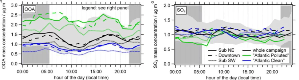
Fig. 6. Diurnal cycles (hourly median values) for OOA (left) and SO4(right) at all sites for the whole campaign, and for “Atlantic Polluted” and “Atlantic Clean” air masses separately. The time period between sunset and sunrise is shaded in grey. Percentiles (25 and 75 %) are shown in light grey exemplarily for the measurements at Sub NE only (whole campaign).
for “Central Europe” and “Atlantic Polluted” air masses, but lower for “Atlantic Clean” air masses. This is especially visi-ble at the Downtown site, while at Sub NE, this is observavisi-ble only for some species (especially HOA). For Sub SW, no averages for “Central Europe” air masses are available due to instrumental downtimes. These differences of the primary emission tracer concentrations for the different air masses cannot be due to air mass origin or spatial distribution of lo-cal sources, since then rather the two “Atlantic” air masses would show similar concentrations of primary emission trac-ers than “Central Europe” and “Atlantic Polluted”. This be-haviour can rather be explained by the higher average wind speed which was observed during the “Atlantic Clean” air masses, which leads to a larger dilution of primary emissions and consequently to lower concentrations of the associated tracers compared to the situation for the other two air masses. Therefore, in our case, wind speed seems to be the dominat-ing factor for the averages of primary emission tracers ob-served at a given site.
For a given air mass, average concentrations of primary emission tracers generally are different for the three measure-ment sites. This is due to the different exposure of the sites to primary emissions, as described above, and in addition due to the different influences of advected emissions from the whole agglomeration, as discussed in Sect. 3.5. In contrast, for
sec-ondary species OOA, SO4, NO3, and NH4, within the
uncer-tainties the same average mass concentrations are observed at all sites for a given type of air mass. A similar distribution
is found for O3. This seems to indicate a more regionally
ho-mogeneous distribution of these secondary species over the greater Paris region, rather than a distribution dominated by local production. This conclusion is backed up by a back-ground measurement case study using the Mobile Labora-tory, which is presented in Sect. 3.4.
Inorganic species: at all sites, comparable average mass
concentrations for inorganic species (SO4, NO3, NH4)were
measured during both “Atlantic” air masses, but much higher mass concentrations were found when “Central Europe” air masses were advected. Here, origin of air mass rather than
local conditions seems to be the dominating factor that deter-mines the pollutant concentrations. The regional character of SO4is also reflected in its diurnal cycle (Fig. 6), which shows
no or only a very small diurnal trend for any of the sites and air masses. This lack of differences between the two types
of “Atlantic” air masses in SO4 diurnal cycles and average
mass concentrations indicates that the relatively short resi-dence times over land for both of these air masses are (in the absence of cloud processing) not sufficiently long to
gener-ate SO4from precursor gases that were picked up (Seinfeld
and Pandis, 2006). This is also supported by the fact that the
measured average SO4mass concentrations for “Atlantic” air
masses of about 1 µg m−3are typical for anthropogenically
influenced marine air masses without significant continen-tal influence, as it was measured with the AMS in several
European coastal regions. For example, SO4 mass
concen-trations of 1.15 µg m−3 for continental marine aerosol were
measured in early summer 2008 at Mace Head (Dall’Osto
et al., 2010a, b), and 0.91 µg m−3 of SO4 were measured
for marine aerosol in late autumn 2008 at the southern coast of Spain (Diesch et al., 2012). This aerosol is not necessar-ily of biogenic origin, as for pristine regions, much lower particulate sulphate mass concentrations have been reported, e.g., 0.18 µg m−3in clean South Atlantic regions (Zorn et al.,
2008). Therefore, a large extent of this aerosol is likely due to e.g. ship emissions and other anthropogenic sources.
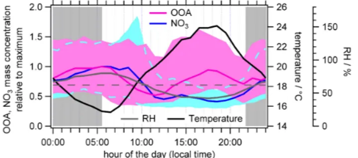
The diurnal cycle of NO3, on the other hand, is driven both
by the temperature and RH dependence of the
gas-particle-partitioning of NH4NO3(Fig. 7). Again, average mass
con-centrations are much higher for the “Central Europe” air masses than for the “Atlantic” air masses. Differences in mass concentrations between the two “Atlantic” air masses
would be much more likely to expect for NO3than for SO4,
as NO3 forms much faster from precursor gases (Seinfeld
and Pandis, 2006). However, due to the very low measured mass concentrations, no significant differences can be found
between the two types of air masses. The same holds for O3
and for NH4, which neutralizes SO4and NO3almost fully