HAL Id: hal-02168170
https://hal.archives-ouvertes.fr/hal-02168170
Submitted on 3 Aug 2020
HAL is a multi-disciplinary open access
archive for the deposit and dissemination of
sci-entific research documents, whether they are
pub-lished or not. The documents may come from
teaching and research institutions in France or
abroad, or from public or private research centers.
L’archive ouverte pluridisciplinaire HAL, est
destinée au dépôt et à la diffusion de documents
scientifiques de niveau recherche, publiés ou non,
émanant des établissements d’enseignement et de
recherche français ou étrangers, des laboratoires
publics ou privés.
ocean chlorophyll product
H. Lavigne, F. d’Ortenzio, Hervé Claustre, A. Poteau
To cite this version:
H. Lavigne, F. d’Ortenzio, Hervé Claustre, A. Poteau. Towards a merged satellite and in situ
fluores-cence ocean chlorophyll product. Biogeosciences, European Geosciences Union, 2012, 9 (6),
pp.2111-2125. �10.5194/bg-9-2111-2012�. �hal-02168170�
www.biogeosciences.net/9/2111/2012/ doi:10.5194/bg-9-2111-2012
© Author(s) 2012. CC Attribution 3.0 License.
Biogeosciences
Towards a merged satellite and in situ fluorescence ocean
chlorophyll product
H. Lavigne1,2, F. D’Ortenzio1,2, H. Claustre1,2, and A. Poteau1,2
1Laboratoire d’Oc´eanographie de Villefranche, CNRS, UMR7093, 06230 Villefranche-sur-Mer, France 2Universit´e Pierre et Marie Curie-Paris 6, UMR7093, Laboratoire d’Oc´eanographie de Villefranche, 06230 Villefranche-sur-Mer, France
Correspondence to: H. Lavigne (heloise.lavigne@obs-vlfr.fr)
Received: 2 November 2011 – Published in Biogeosciences Discuss.: 13 December 2011 Revised: 3 May 2012 – Accepted: 3 May 2012 – Published: 12 June 2012
Abstract. Understanding the ocean carbon cycle requires a precise assessment of phytoplankton biomass in the oceans. In terms of numbers of observations, satellite data represent the largest available data set. However, as they are limited to surface waters, they have to be merged with in situ observa-tions. Amongst the in situ data, fluorescence profiles consti-tute the greatest data set available, because fluorometers have operated routinely on oceanographic cruises since the 1970s. Nevertheless, fluorescence is only a proxy of the total chloro-phyll a concentration and a data calibration is required. Cal-ibration issues are, however, sources of uncertainty, and they have prevented a systematic and wide range exploitation of the fluorescence data set. In particular, very few attempts to standardize the fluorescence databases have been made. Con-sequently, merged estimations with other data sources (e.g. satellite) are lacking.
We propose a merging method to fill this gap. It consists firstly in adjusting the fluorescence profile to impose a zero chlorophyll a concentration at depth. Secondly, each point of the fluorescence profile is then multiplied by a correction coefficient, which forces the chlorophyll a integrated con-tent measured on the fluorescence profile to be consiscon-tent with the concomitant ocean colour observation. The method is close to the approach proposed by Boss et al. (2008) to correct fluorescence data of a profiling float, although im-portant differences do exist. To develop and test our ap-proach, in situ data from three open ocean stations (BATS, HOT and DYFAMED) were used. Comparison of the so-called “satellite-corrected” fluorescence profiles with con-comitant bottle-derived estimations of chlorophyll a concen-tration was performed to evaluate the final error (estimated at
31 %). Comparison with the Boss et al. (2008) method, using a subset of the DYFAMED data set, demonstrated that the methods have similar accuracy. The method was applied to two different data sets to demonstrate its utility. Using fluo-rescence profiles at BATS, we show that the integration of “satellite-corrected” fluorescence profiles in chlorophyll a climatologies could improve both the statistical relevance of chlorophyll a averages and the vertical structure of the chlorophyll a field. We also show that our method could be efficiently used to process, within near-real time, profiles ob-tained by a fluorometer deployed on autonomous platforms, in our case a bio-optical profiling float. The application of the proposed method should provide a first step towards the generation of a merged satellite/fluorescence chlorophyll a product, as the “satellite-corrected” profiles should then be consistent with satellite observations. Improved climatolo-gies with more consistent satellite and in situ data are likely to enhance the performance of present biogeochemical mod-els.
1 Introduction
In the ocean, chlorophyll a concentration (the sum of chloro-phyll a (Chl a), divinyl chlorochloro-phyll a and chlorochloro-phyllide a) is considered a good, although not optimal, proxy for phy-toplankton biomass (e.g. Cullen, 1982; Strickland, 1965). Considering the key role of phytoplankton in the global car-bon cycle, understanding the Chl a concentration (“Chl aC”) spatio-temporal distribution and variability is of primary im-portance for modern oceanography (Claustre et al., 2010).
Although it is the most abundant biological oceanic mea-surement, Chl aCobservations are, however, scarce, particu-larly in comparison with the number of physical observations available (e.g. temperature and salinity). Among the three main approaches that exist for measuring Chl aC(i.e. water sampling, ocean colour and induced fluorescence; see later), fluorescence is the only one that has not been included in global re-analysis, as, for example, open ocean climatologies of Chl aC(Gregg and Conkright, 2001). However, it repre-sents the most important source of in situ data in terms of numbers of observations (i.e. 36 707 profiles in the World Ocean Database 2009; Boyer et al., 2009), and this trend is likely to increase in the near future given the recent develop-ment of autonomous platforms equipped with fluorometers. Combining fluorescence profiles with other data (i.e. ocean colour and sampling bottles) should strongly enhance our knowledge of the spatio-temporal variability of the Chl aC, and consequently, improve our understanding of the phyto-plankton dynamics.
The conventional and historical approach to measure Chl aC in the ocean is to filter water samples collected at different depths, which are further analysed using three prin-cipal benchtop methods: fluorometry (Holm-Hansen et al., 1965), spectrophotometry (Lorenzen, 1967) and chromatog-raphy (Mantoura and Llewellyn, 1983). The three techniques have different accuracy and precision. A general consensus indicates that the most accurate method is high performance liquid chromatography (HPLC, Gieskes and Kraay, 1983; Hooker et al., 2009), which provides the concentrations of a large spectrum of phytoplankton accessory pigments in ad-dition to Chl aC.
There are also bio-optical techniques that offer alternative methods to obtain Chl aC in the ocean. The peak of par-ticulate absorption between 650 nm and 715 nm is a signa-ture of Chl a absorption and can be used to derive Chl aC (Davis et al., 1997; Boss et al., 2007). Absorption of par-ticulates is obtained from in-situ total absorption measure-ments corrected for pure water and coloured dissolved ma-terial absorption. Moreover, empirical relationships, relating the gradients in light field to in-water compounds, were de-veloped to estimate Chl aCfrom radiometers that measure light intensity in the visible spectrum (Morel, 1988). Simi-larly, bio-optical relationships were successfully developed to obtain Chl aC from satellite-mounted radiometers. The satellite-derived maps provide a unique temporal and spa-tial picture of the Chl aC at global scale (Feldman et al., 1989; McClain et al., 1998). However, satellite observations are limited to the ocean surface and their error on Chl aC, calculated by match-up analysis of concurrent satellite and HPLC measurements, was evaluated to vary around ±35 % in the open ocean (Bailey and Werdell, 2006; Moore et al., 2009).
Bio-optical approaches based on fluorescence techniques (Lorenzen, 1966) provide another method to evaluate Chl aC. Irradiated by blue light, Chl a absorbs and re-emits, in the red
part of the spectrum, a quantity of light that is proportional to a∗·Chl aC, where a∗is the chlorophyll-specific absorption
coefficient. Based on this concept, instruments inducing and measuring fluorescence (i.e. fluorometers) provide a robust method to estimate in situ Chl aCwith a non-invasive tech-nique. Additionally, the acquisition frequency of fluorome-ters (up to 8 Hz), and their possible connection with a CTD probe, allows for winch-based deployment and the collection of vertically continuous profiles of fluorescence. Although calibration issues still prevent a wide scientific exploitation of fluorescence profiles (see later), during the last 30 yr they have been extensively collected, becoming a standard mea-surement in oceanography.
The calibration of fluorometers is a complex process. Manufacturer calibration is often too simplistic to meet sci-entific requirements, and calibration needs to be regularly verified, due to lamp and sensor performance degradation with time. However, the most problematic issues are the high variability and nonlinearity of the fluorescence/Chl aC relationship (Falkowski and Kiefer, 1985; Kiefer, 1973). Changes in environmental conditions (e.g. light intensity, nu-trient availability) can induce modifications in taxonomic as-semblages or in physiological states of phytoplankton, with an impact on the fluorescence to Chl aCratio (Cullen, 1982; Althuis et al., 1994; Claustre et al., 1999; Cleveland and Perry, 1987; Loftus and Seliger, 1975). As mentioned above, fluorescence is not directly proportional to Chl aC but to
a∗·Chl aC. Yet, a∗strongly varies, especially because of the packaging effect, which induces a decrease in a∗in response to an increase in the size of the phytoplankton cell and/or an increase in the Chl aCcontent per cell (Morel and Bricaud, 1981). Consequently, a∗changes with the community
com-position and with the light intensity, which decreases with depth. Another source of variability for the fluorescence to Chl aCratio is the non-photochemical quenching (NPQ) of fluorescence, particularly relevant in the surface layers. NPQ occurs when, in response to supra-optimal light irradiation, phytoplankton triggers photo-protection mechanisms, induc-ing a drastic decrease of the fluorescence to Chl aC ratio (Kolber and Falkowski, 1993; M¨uller et al., 2001). The final effect of NPQ is a decrease of fluorescence at the surface, not paralleled by a Chl aCdiminution (Xing et al., 2011; Sack-man et al., 2008; Cullen and Lewis, 1995). An in situ calibra-tion of the fluorometers is generally carried out at the time of deployment, using Chl aCobtained from water samples col-lected during the fluorescence profiles acquisition and fur-ther analyzed with HPLC or spectrofluorometer (Cetinic et al., 2009; Sharples et al., 2001; Strass, 1990). This opera-tion, however, is not systematically carried out. Moreover, even when bottle data are available, they are often recorded in a different database to the fluorescence profiles. During oceanographic cruises, in situ fluorescence profiles are gen-erally used to indicate a “generalized” biomass index (Strick-land, 1968) and then interpreted to decide the depths for bottle sampling. Occasionally, they are used to improve the
interpolation between discrete Chl aC estimations (see, for example, Morel and Maritorena, 2001). However, extensive and global analyses, including several data sets of fluores-cence profiles, obtained by different fluorometers, are lack-ing.
The main consequence of this situation is that fluores-cence data are underused. The constraints of calibration hin-der any combination of the different fluorescence data sets and also prevent their merging with other data sources. No fluorescence profile has been integrated, for example, in ex-isting Chl aCclimatologies (Conkright et al., 2002), which are exclusively based on Chl aCestimations obtained from water sample data (HPLC or spectrofluorometer measure-ments). Consequently, climatologies are strongly interpo-lated, as the initial data density is generally low (Conkright et al., 2002). Furthermore, existing methods to generate blended Chl aCproducts combining data derived from differ-ent methods generally exclude fluorescence data. They have been limited to the merging of ocean colour satellite observa-tions with water sample-derived estimaobserva-tions. A pure blend-ing method (Gregg and Conkright, 2001) was developed to directly merge satellite and in situ data. A more indirect ap-proach used satellite and in situ data to establish empirical relationships between the surface Chl aCand its vertical sig-nature (Morel and Berthon, 1989; Uitz et al., 2006), in order to reconstruct a vertical profile for each available satellite pixel. Surprisingly, no attempt yet has been made to merge fluorescence profiles with alternative Chl aC measurement approaches.
In summary, the lack of standardization of the fluorescence calibration methods prevents the development of a merged procedure that makes use of a number of different fluores-cence data sets and of their combination with other data sources.
Recent approaches were presented, based on ancillary data (e.g. simultaneous irradiance profiles, Xing et al., 2011), on the shape of fluorescence profile (Mignot et al., 2011) or on satellite ocean colour Chl aCobservations (Boss et al., 2008). The last method (Boss et al., 2008), although developed to correct a profiling float fluorometer, also points to a reliable way to merge fluorescence profiles and satellite observations. However, the Boss et al. (2008) approach, in its present form, was developed to be applied to a time series of profiles per-formed by a single fluorometer deployed on a profiling float and is likely not suitable for other data sets. Indeed, a unique set of correction factors was calculated for the whole lifetime of the profiling float. Consequently, although the re-adjusted data are generally consistent with the satellite, the computa-tion of a unique set of correccomputa-tion factors implies that some profiles could be erroneously corrected. In the framework of a combined satellite-fluorescence profile product, the present form of the Boss et al. (2008) method could then be modified in order to be applied on a single profile basis.
Here, we propose a method to merge fluorescence profiles and satellite ocean colour observations, which is
conceptu-ally close to the Boss et al. (2008) procedure. The main dif-ference is that it is applicable on a single profile basis. Con-sequently, each profile will be characterized by a specific set of correction factors and the obtained Chl aCprofiles would be strictly consistent with the satellite estimation measured in the same place and at the same time.
We developed and tested the merging method on three long-term time series of simultaneous observations of fluo-rescence profiles and Chl aCobtained from HPLC analysis. Fluorescence profiles and satellite data were matched and combined to generate Chl aCprofiles. Finally, the obtained profiles were compared with concomitant HPLC Chl aC, to test the method performances. Additionally, performance in-dexes of the present merging method were compared to the Boss et al. (2008) method performances on a subset of DY-FAMED data. The different sources of error influencing the accuracy of the merged profiles were then discussed. Finally, two examples of application were presented: the production of a monthly Chl aCclimatology using fluorescence profiles and the treatment of a time series of fluorescence profiles recorded by a fluorometer deployed on a profiling float. The two applications demonstrate the capacity of the method to enhance the consistency of the fluorescence data set with other Chl aCdata sources available. Consequently, they rep-resent a first step towards merged Chl aCestimations.
2 Data
In situ data from the long-term time series data sets of sta-tions BATS (Michaels and Knap, 1996, in the Sargasso Sea), DYFAMED (Marty et al., 2002, in the northwestern Mediter-ranean Sea) and HOT (Karl and Lukas, 1996, in the North Pacific) were used over the 1998–2007 period (i.e. the pe-riod of activity of the SeaWiFS ocean colour sensor). For each station, fluorescence, temperature and salinity profiles were extracted, as well as HPLC Chl aCderived from dis-crete samples, when available.
Surface Chl aC over the three sites was derived from the 8-day images at 9 km spatial resolution from the Sea-WiFS satellite ocean colour sensor, which constitutes the longest temporal series of ocean colour observations (Mc-Clain, 2009). For each available fluorescence profile, the satellite image that matched the date of the profile was se-lected, and a Chl aCaverage was calculated in a ±0.1◦by
±0.1◦ sized box centred on the profile geographical
posi-tion (i.e. “fluo” match-up). A “fluo” match-up was retained, if more than 30 % of pixels were available in the box.
For each station, an additional satellite match-up analysis was performed by extracting ocean colour data when HPLC observations were available (“HPLC” match-up). To verify the sensitivity of the match-up analysis to the size of the temporal and spatial windows, near surface Chl aC from HPLC profiles (computed as described in Morel and Berthon, 1989) was compared to satellite observations extracted from
SeaWiFS images at both 8-day and 1-day temporal resolu-tion and on spatial boxes of ±0.25◦ and ±0.1◦dimensions
(Table 1). Increasing temporal and spatial resolutions does not significantly modify the similarity between the HPLC and satellite estimations (tests of similarity on absolute per-cent difference: 8-day ±0.25◦ with 8-day ±0.1◦ p-value = 0.86; 8-day ±0.25◦with 1-day ±0.25◦p-value = 0.66). How-ever, the number of match-ups strongly decreased. Based on these tests, carried out on the “HPLC” match-ups, the “fluo” match-up procedure was then performed using the 8-day res-olution products and the ±0.1◦square boxes.
In the BATS and DYFAMED HPLC data sets, the lowest Chl aCwas around 0.001 mg m−3, whereas at the HOT sta-tion lowest concentrasta-tions were about 0.01 mg m−3. As ob-servations showed that, in the most oligotrophic regions of the global ocean, Chl aCat the surface is about 0.02 mg m−3 (Ras et al., 2008), very low Chl aC(<0.01 mg m−3)should correspond to deep measurements that are not relevant to this present study. Consequently, to standardize the data sets, we eliminated all the HPLC measurements <0.01 mg m−3.
On the HPLC profiles, negative spikes (2 % of total HPLC data points) and incomplete profiles (i.e. less than 5 points, 2.2 % of available profiles) were also removed. An additional quality control procedure (D’Ortenzio et al., 2010) was ap-plied to the fluorescence profiles, which checked for outliers, spikes and unexpected gradients. Finally, an additional vi-sual control allowed for the identification of altered profiles, which were removed.
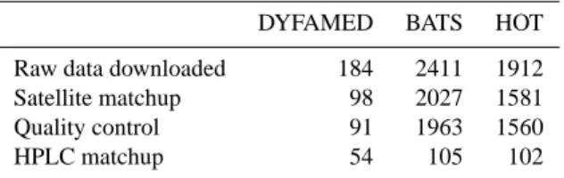
After this processing, the fluorescence database was com-posed of 3614 profiles, all with an associated satellite ocean colour Chl aC estimation: 91 at DYFAMED, 1560 at HOT, 1963 at BATS (see Table 2 for a summary of the available data).
3 Method
3.1 Overview
The common procedure to convert a fluorescence profile (FLUO) into Chl aC(Boss et al., 2008; Cetinic et al., 2009; Xing et al., 2011) can be formalised by
Chl aC=α(FLUO − β). (1)
The β parameter indicates the response of the instrument in the absence of signal, and it is commonly computed by blocking the sensor window. The α coefficient is initially provided by the manufacturer, and it is calculated by linear regression with samples at fixed and known Chl aC. Post-processing evaluation of the α parameter can be carried out by regressing fluorescence profiles with in situ Chl aC ob-tained by HPLC or fluorometric water sample analyses. The post-processing adjustment is generally more accurate than the manufacturer calibration, as it is often carried out in nat-ural conditions and on a greater number of data points.
How-Table 1. Sensitivity study on the impact of the resolution of the
satellite extraction window of “HPLC” match-up. The number (N ) and the percentage of valid match-ups, the median percent differ-ence (MPD) between satellite and in-situ data as well as the deter-mination coefficient (r2)of the regression performed between two data sets are reported.
Temporal Spatial Percentage of
resolution resolution valid match-ups MPD r2 N
8 days ±0.25◦ 80.5 % 32 % 0.62 267 8 days ±0.1◦ 77.5 % 34 % 0.63 256 1 day ±0.25◦ 18.5 % 36 % 0.43 56
Table 2. Quantity of fluorescence profiles available after each step
of the data processing.
DYFAMED BATS HOT Raw data downloaded 184 2411 1912 Satellite matchup 98 2027 1581 Quality control 91 1963 1560 HPLC matchup 54 105 102
ever, it requires the analysis of water samples, which are not always available.
Here, we evaluated the β parameter by considering fluo-rescence measurements at depth, where Chl aCis supposed to be zero, whereas the α parameter was estimated for each fluorescence profile from a simultaneous ocean colour obser-vation.
The evaluation of the α parameter was based on the as-sumption that the near-surface Chl aC, chlsurfCin mg m−3, and the integrated Chl a biomass across k times the euphotic depth hchlik·Ze in mg m
−2, (k = 1 or k = 1.5) are related (Eq. 2; Morel and Berthon, 1989; Uitz et al., 2006). The eu-photic depth is defined as the depth at which light intensity falls to 1 % of its value at the surface.
hchlik·Ze=AchlsurfC
B
(2)
In Eq. (2), A, expressed in meters, and B, dimensionless, are coefficients that were determined by regressions carried out on in situ data (Uitz et al., 2006). They have different values depending on whether the water column is stratified or not.
3.2 Parameters computation
Following Morel and Berthon (1989) and Uitz et al. (2006), the discrimination between a stratified or mixed water col-umn was determined according to the ratio between the depth of the euphotic layer (Ze)and the depth of the mixed layer (Zm). The water column was assumed to be mixed when
Ze/Zm<1 and stratified when Ze/Zm>1. Zm was evalu-ated from potential density profiles using a density criterion of 0.03 kg m−3(de Boyer Montegut et al., 2004; D’Ortenzio
et al., 2005). Ze was determined with the following proce-dure: (1) the attenuation coefficient at 490 nm, Kd490, from the satellite-derived Chl aC (Morel and Maritorena, 2001); (2) the total attenuation coefficient, Kd,PAR, from Kd490 (Rochford et al., 2001); (3) finally, Ze was retrieved from
Kd, PAR, using the equations of exponential decrease of light
over depth.
Before computing the α and β parameters, fluorescence profiles were corrected for non-photochemical quenching (NPQ). Although NPQ represents a serious issue for the fluo-rescence calibration (Cullen and Lewis, 1995), methods exist to evaluate, and if possible correct, the NPQ impact on the Chl aCto fluorescence ratio (Sackmann et al., 2008; Xing et al., 2012). The most complex approaches (i.e. Sackmann et al., 2008; Behrenfeld and Boss, 2006) provided fluorescence corrections on the basis of (1) other proxies for phytoplank-ton (i.e. optical backscattering) or (2) night light fluorescence profiles, which are not affected by NPQ. Here, we applied the method of Xing et al. (2012), which only requires mixed layer depth as input parameters to provide an NPQ correc-tion. This method consists in extrapolating up to the surface the highest fluorescence value encountered within the mixed layer, identified after a smoothing of the profile (median fil-ter) to reduce the noise in fluorescence data. Although this method is less sophisticated than other approaches, its large range of applicability (i.e. only mixed layer depth is required as auxiliary parameter) better matches with the rationale of our approach, which is to develop a robust method to merge satellite and fluorescence profiles. Additionally, the use of the whole 1.5 Zelayer instead of only surface records to cor-rect fluorescence allows for a minimization of the error that would be induced by a wrong NPQ parameterization. To as-sess the relevance of the Xing et al. (2012) NPQ correction in the present merging method, we used the 776 pairings of matchup points located in mixed layer for the three data sets tested, obtaining a median ratio of re-adjusted fluorescence to HPLC data of 0.93, if the Xing et al. (2012) NPQ correc-tion was previously applied and 0.78 if it was not. A Student test to compare re-adjusted fluorescence with HPLC ratios in the two conditions (i.e. with and without quenching correc-tion) reveals that the positive effect of the Xing et al. (2012) NPQ correction is significant (p-value < 0.01).
The coefficient β was evaluated under the hypothesis that Chl aCwas equal to zero in deep waters:
β =average (FLUO(z)), for z > Zthreshold (3) where z is the depth in meters and Zthreshold is a depth be-low, where the Chl aC was considered null. Here, we as-sumed that Zthreshold=300 m for stratified water columns, and Zthreshold=Zm +100 m for mixed water columns.
The α parameter for each fluorescence profile was, sub-sequently, determined thanks to ocean colour satellite mea-surements. First, using Eq. (2) and the coefficients of Uitz et al. (2006), the near-surface Chl aC, measured by satellite sen-sor, was related to the integrated Chl a content over 1.5Ze,
hchli1.5Ze(Morel and Berthon, 1989; Uitz et al., 2006). Then,
the fluorescence profile, corrected for NPQ effect, was ad-justed so that hchli1.5Ze, computed from Uitz et al. (2006)
coefficients (see Table 4 in Uitz et al., 2006), and the in-tegrated Chl a, measured by fluorescence, coincide. α was accordingly computed as followed:
α = hchl1.5Zei
R1.5Ze
0 (FLOU(z) − β)dz
. (4)
Note that we used integrated content over 1.5Ze, because it is recognized that important Chl aC is often present below the euphotic layer (Uitz et al., 2006).
The estimation of the parameters α and β was carried out for each available fluorescence profile of the three sta-tions, and, using Eq. (1), ocean colour/fluorescence merged profiles were finally obtained (thereafter “satellite-corrected” profiles).
3.3 Statistics used to assess method performances To evaluate the method, various statistics were computed on couples of concomitant Chl aCderived from both “satellite-corrected” profiles and HPLC estimations, the last being con-sidered as the “true” value. The two series of Chl aC esti-mations (i.e. “satellite-corrected” and HPLC) were matched according to the station, the sampling day and the depth. All couples of data with an HPLC-derived Chl aCgreater than 0.01 mg m−3were used for validation. Points located below the 1.5Zelayer represent 18 % of the validation data set.
The median value of ratio “satellite-corrected” to HPLC Chl aC estimations points to the overall bias. The semi-interquartile range (SIQR) provides insight on the spreading of data and it is defined as
SIQR =Q3−Q1
2 (5)
where Q1is the 25th percentile and Q3is the 75th percentile of each series of “satellite-corrected” to HPLC ratio.
The median percent difference (MPD) was calculated to measure how accurately the Chl aCvalues of the “satellite-corrected” profiles agree with HPLC measurements. It is de-fined as the median of the individual absolute percent differ-ences (PD), computed as
PDi=100
|Xi−Yi| Yi
(6)
where Yi is the Chl aCmeasured with HPLC of the i-th
vali-dation point and Xiis the corresponding “satellite-corrected”
value. The determination coefficients (r2)of type I linear regression between “satellite-corrected” and HPLC estima-tions were also evaluated.
a − BATS 0.001 0.01 0.1 1 0.001 0.01 0.1 1 b − DYFAMED 0.001 0.01 0.1 1 0.001 0.01 0.1 1 c − HOT 0.001 0.01 0.1 1 0.001 0.01 0.1 1 d − Surface points 0.001 0.01 0.1 1 0.001 0.01 0.1 1 Chl a
C from "satellite−corrected" fluorescence
Chl aC from HPLC
Fig. 1. Scatter plots of “satellite-corrected” Chl aCas a function of
concomitant HPLC Chl aC, in mg m−3. Colours characterize the er-ror of satellite in the estimation of near surface Chl aC: overestima-tion exceeding 35 % (red), underestimaoverestima-tion exceeding 35 % (blue) and error inferior to ±35 % (green). Only surface points above 20 m depth are displayed in (d).
4 Results
4.1 Method performances
The four terms (i.e. median “satellite-corrected” to HPLC ratio, SIQR, MPD and r2)described in Sect. 3.3 were cal-culated for complete data sets of 2591 pairings of concur-rent “satellite-corrected” with HPLC Chl aC (491 for DY-FAMED, 987 for BATS and 1113 for HOT). Because of the log-normal distribution of Chl aC, values were log-transformed (Campbell, 1995) prior to statistical analysis, except for the PD calculation.
Statistics and scatter plots are shown in Table 3 and Fig. 1, for each station. Figure 2 shows some examples of the ini-tial fluorescence profiles, with their corresponding “satellite-corrected” and HPLC profiles. In Fig. 2, the satellite sur-face Chl aC used for merging is also depicted, as well as the “HPLC-calibrated” profiles, computed by adapting the initial fluorescence profiles to the simultaneously available discrete HPLC observations (following the method of Morel and Maritorena, 2001).
The scattering of data for the three stations is relatively ho-mogenous for values higher than 0.05 mg m−3along the 1:1 line for each station (Fig. 1a to c) and also for surface data (<20 m, Fig. 1d), suggesting that the NPQ-correction applied here was globally efficient. The present merging method does not appear biased, as median values of the
“satellite-Table 3. Comparison of “satellite-corrected” Chl aC with
con-comitant HPLC values. The median “satellite-corrected” to HPLC Chl aCratio, the semi-interquartile range (SIQR) measured on the previous series of ratio, the median percent difference (MPD) be-tween “satellite-corrected” and HPLC data, as well as determina-tion coefficient (r2)of the regression performed between “satellite-corrected” and HPLC data points are reported. N indicates the num-ber of couples of data points available.∗refers to the variables that were calculated on log-transformed data.
Median ratio∗ SIQR* MPD (%) r2∗ N
total 1.02 0.17 31.4 0.68 2591 DYFAMED 0.95 0.30 41.2 0.70 491 BATS 1.02 0.15 29.3 0.67 987 HOT 1.04 0.16 29.4 0.63 1113
corrected” to HPLC ratio are within 5 % of a unit (Table 3). An important scatter, especially at the DYFAMED station, is, however, observed with SIQR, ranging from 0.15 to 0.30. The MPD ranges from 29 % for stations BATS and HOT to 41 % for DYFAMED, with an overall median value of 31 %. Determination coefficients range from 0.63 for HOT to 0.70 for DYFAMED station. Not surprisingly, r2is higher when large ranges of Chl aCare observed (i.e. DYFAMED). From performances statistics, the DYFAMED station ap-pears likely different from BATS and HOTS, which showed similar performances. An explication of this difference could be ascribed to the phytoplankton variability, which at DY-FAMED is characterized by a marked seasonality, determin-ing a large phytoplankton biodiversity (Marty et al., 2002). Additionally, a strong interannual variability is observed at DYFAMED, with irregular succession of blooming and non-blooming years (Bosc et al., 2004). All the above could in-duce a higher variability of the Chl aCto fluorescence ratio, which likely influences the performances of our approach.
The impact of the error of satellite observations on the “satellite-corrected” profiles is different for the three test sta-tions analyzed (Table 4). At DYFAMED and BATS, the er-ror of the “satellite-corrected” profiles (when compared with HPLC estimations) is largest when the difference between satellite and HPLC surface values is greater than ±35 % (Ta-ble 4; the 35 % threshold value has been used, because it is the accepted averaged error of the satellite chlorophyll, Mc-Clain, 2009; Moore et al., 2009). Conversely, at the HOT station, the final error appears to be hardly affected by the accuracy of the satellite observations.
A comparison of the vertically integrated Chl aCwas also performed (Fig. 3). Chl aCof both “satellite-corrected” and “HPLC-calibrated” profiles was integrated over 200 m depth, which generally corresponds to the deepest HPLC observa-tion. Moreover, at 200 m depth, Chl aCis in most cases con-sidered to be close to zero. For the integrated Chl aC, the median of “satellite-corrected” to “HPLC-calibrated” ratio is 1.02, SIQR is 0.23 and median error is 21 %. Determination
Chl aC (mg m−3) depth (m) 0.0 0.1 0.2 0.3 0.4 250 200 150 100 50 0 ●● ● ● ● ● ● ● ● ● ● ● * a BATS 1999−07−06 Chl aC (mg m−3) depth (m) 0.0 0.1 0.2 0.3 0.4 250 200 150 100 50 0 ● ● ● ● ● ● ● ● ● ● ● ● * b BATS 2004−10−13 Chl aC (mg m−3) depth (m) 0.0 0.5 1.0 1.5 250 200 150 100 50 0 ●● ● ● ● ● ● ● ● ● ● ● * c DYFAMED 2000−03−28 Chl aC (mg m−3) depth (m) 0.0 0.2 0.4 0.6 0.8 1.0 250 200 150 100 50 0 ● ● ● ● ● ● ● ● ● * d DYFAMED 2001−04−27 Chl aC (mg m−3) depth (m) 0.0 0.1 0.2 0.3 0.4 0.5 0.6 0.7 250 200 150 100 50 0 ● ● ● ● ● ● ● ● ● ● ● ● * e HOT 2005−07−17 Chl aC (mg m−3) depth (m) 0.0 0.2 0.4 0.6 0.8 250 200 150 100 50 0 ● ● ● ● ● ● ● ● ● ● ● ● * f HOT 2001−12−15
Fig. 2. Examples of “satellite-corrected” profiles (black solid line),
“HPLC-calibrated” profiles (grey solid line), factory-calibrated flu-orescence profiles (black dashed line) and, only for DYFAMED ex-amples, “Boss-calibrated” profiles (black dotted lines). As a com-plement, HPLC data points are indicated by grey circles and satellite surface Chl aCby black stars.
coefficient in the regression model only reaches 55 %, in-dicating a relatively weak coherence between the data sets, which is particularly evident for low values. Again, satel-lite accuracy does impact the final result. Underestimation (overestimation) of the satellite surface Chl aC directly re-sults in an underestimation (overestimation) of the integrated content of the “satellite-corrected” profiles. Nevertheless, the impact is less relevant than expected: of the 129 profiles with an error on satellite Chl aChigher than 35 %, more than half (82 profiles) showed integrated chlorophyll contents close to their corresponding HPLC-calibrated profiles (error less than 35 %).
Finally, we compared the euphotic depths calculated from the “satellite-corrected” and from the “HPLC-calibrated” profiles, following the method of Morel and Berthon (1989) but with the parameterisation of Morel and Maritorena
● ● ● ● ● ● ● ● ● ● ● ● ● ● ● ● ● ● ● ● ● ● ● ● ● ● ● ● ● ● ● ● ● ● ● ● ● ● ● ● ● ● ● ● ● ● ● ● ● ● ● ● ● ● 10 20 50 100 200 10 20 50 100 200
Integrated content in Chl a measured on "HPLC−calibrated" profiles
Integr
ated content in Chl
a
measured on "satellite−corrected" profiles
●
BATS DYFAMED HOT
Fig. 3. Scatter plot of integrated Chl a content over 200 m
com-puted on “satellite-corrected” profiles, as a function of integrated Chl a content computed on “HPLC-calibrated” profiles. Both Chl a contents are expressed in mg m−2. Similarly to Fig. 1, colour code refers to the error of satellite in the estimation of near-surface Chl aC.
Table 4. Impact of the satellite Chl aC accuracy on the error of
final corrected profiles. The satellite error was measured with the relative percent difference (rpd) between satellite extracted Chl aC and near surface Chl aC derived from HPLC profiles. The accu-racy of the merging method was assessed with the median absolute percent difference (MPD) between “satellite-corrected” and HPLC data points.
Satellite error rpd < −35 −35 < rpd < 35 rpd > 35 Total
MPD N MPD N MPD N MPD
DYFAMED 60.5 27 36.9 161 40.4 303 41.2
BATS 32.4 72 24.4 455 35.8 460 29.3
HOT 32.1 140 28.6 715 29.3 258 29.4
(2001, Fig. 4). Note that the euphotic depth is an impor-tant parameter of our approach, since it was used to evaluate the layer of integration in Eq. (4) and to establish whether the water column is stratified or mixed. The points are uni-formly scattered around the 1:1 line. Similarly to the analysis of integrated Chl aC, it appears that the satellite error, deter-mined by comparison with concomitant surface HPLC, tends to affect the estimation of Ze in “satellite-corrected” pro-files. However, the correlation between “satellite-corrected” and “HPLC-calibrated” Ze is satisfying (median ratio of “satellite-corrected” to “HPLC-calibrated” = 0.97, SIQR = 0.09, MPD = 9.5 %, r2=0.64).
● ● ● ● ● ● ● ● ● ● ● ● ● ● ● ● ● ● ● ● ● ● ● ● ● ● ● ● ● ● ● ● ● ● ● ● ● ● ● ● ● ● ● ● ● ● ● ● ● ● ● ● ● ● 20 40 60 80 100 120 140 20 40 60 80 100 120 140
Euphotic depth measured on "HPLC−calibrated" profiles
Euphotic depth measured on "satellite−corrected" profiles ●
BATS DYFAMED HOT
Fig. 4. Scatter plot of the euphotic depth computed on
“satellite-corrected” profiles as a function of the euphotic depth computed on “HPLC-calibrated” profiles using the algorithm described by Morel and Berthon (1989). Both euphotic depths are expressed in meters (m). Similarly to Fig. 1, colour code refers to the error of satellite in the estimation of near-surface Chl aC.
4.2 Comparison with the method proposed by Boss et al. (2008)
Even though differences exist, our approach is close to the Boss et al. (2008) fluorescence correction method. Both methods use a satellite reference, except that the Boss et al. (2008) approach uses only surface data to compare with remote sensing and was developed to be applied to a set of fluorescence profiles measured by a unique instrument (i.e. profiling float), free of instrumental drift. To verify the per-formances of both approaches, we selected a subset of data from the DYFAMED data set, in order to be as close as pos-sible to the terms of applicability of the Boss et al. (2008) method (i.e. data obtained by a unique instrument). The DY-FAMED subset of profiles was obtained by a single fluorom-eter from 2000 to 2002. To verify that there was no instru-mental drift during this period, the deep fluorescence values have been checked (i.e. deep values between a standard de-viation from the long-term mean). The resulting subset of DYFAMED data comprises 47 fluorescence profiles, 24 of which were associated with a concomitant HPLC profile.
By definition, the coefficients α and β in the Boss et al. (2008) approach (called αB and βB hereafter) were
con-sidered constant. Using the 47 profiles available, βB was
computed using the median value of the β coefficients com-puted with our method. The αB coefficient was calculated
as the type II regression slope of a regression analysis
per-Table 5. Comparison, on a subset of DYFAMED data, of
“satellite-corrected” and “Boss-calibrated” Chl aCwith concomitant HPLC values. See the caption of Table 3 for details about parameters.
Median ratio∗ SIQR* MPD (%) r2∗ N
Boss et al. (2008) 0.97 0.23 42.1 0.86 213
Present paper 0.92 0.28 41.9 0.78 213
formed between surface satellite Chl aCand the correspond-ing surface values of fluorescence profiles. Note, however, that the satellite Chl aCproduct that we used has different spatial (9 km instead of 1 km in Boss et al., 2008) and tem-poral (8-day instead of 1-day) resolutions.
The comparison of “satellite-corrected” and “Boss-calibrated” profiles (i.e. fluorescence profiles calibrated with the Boss et al., 2008, method) with concomitant HPLC Chl aCestimations (Table 5, 213 validation points) indicates that the performance indexes of both methods are equiva-lent (MPD = 41.9 % with the present method and 42.1 % with the Boss et al., 2008, method). Dispersion is slightly reduced with the Boss et al. (2008) method compared with the present merging method (SIQR = 0.23 against 0.28 with our method and r2=0.86 against 0.78). Also, our merging method seems more sensitive to the accuracy of satellite data (see example in Fig. 2c and d).
4.3 Examples of application 4.3.1 Chlorophyll a climatology
The utilisation of the large data set of fluorescence profiles, once properly adjusted, should strongly improve the existing climatologies.
1. We linearly interpolated the HPLC discrete profiles in the vertical to generate nearly continuous profiles at 1m resolution. Twelve monthly HPLC average values were then calculated over standard depths, defined for each station by considering the most recurrently sam-pled depths. At each standard depth, monthly climato-logical means were also computed by averaging, for a given month, the Chl aCextracted from the “satellite-corrected” profiles. The resulting mean values were finally compared with the HPLC-derived estimations (Fig. 5 and Table 6). Resulting statistics are generally improved (see Table 6): SIQR is 0.11 (instead of 0.16 for the single profile application); MPD is 22 % (in-stead of 31 %) and r2 is 0.82 (instead of 0.67). HPLC to “satellite-corrected” data spreading is also reduced, with most of the points concentrated around the 1:1 line. However, as also observed for the single profile com-parison (Fig. 1), dispersion increases for concentrations lower than 0.05 mg m−3.
Table 6. Comparison between “satellite-corrected” Chl aCand con-comitant HPLC values after having applied a monthly average filter. See the caption of Table 3 for details about parameters.
Median ratio∗ SIQR* MPD (%) r2∗ N
total 1.03 0.11 21.6 0.82 432 DYFAMED 1.03 0.30 33.9 0.80 144 BATS 1.02 0.08 16.3 0.85 144 HOT 1.04 0.10 18.4 0.80 144
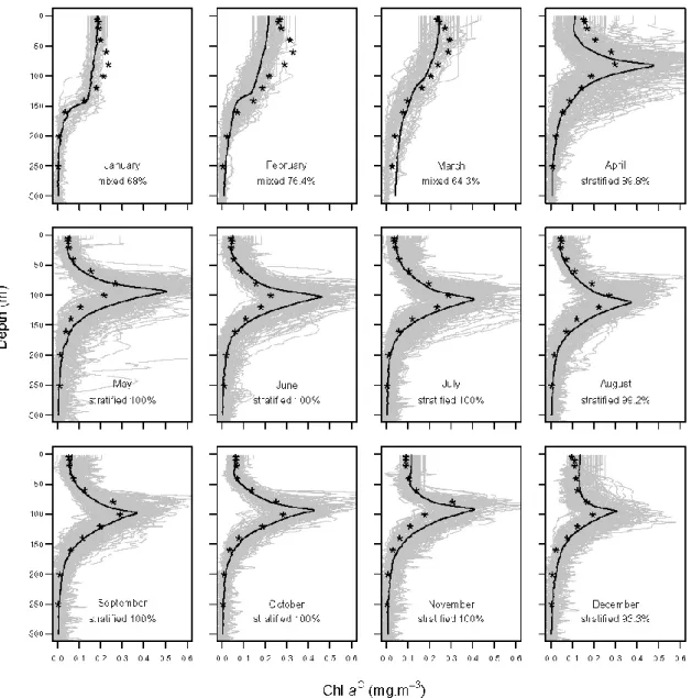
2. The utilisation of “satellite-corrected” profiles led us to envisage new types of climatologies that could better reproduce the vertical distribution of Chl aC. A new procedure is proposed here (see Appendix A for com-putation details). Briefly, the procedure tends to iden-tify, in all available Chl aC profiles, relevant features of the profile, such as the DCM depth, and averages them to reconstruct a climatological profile, which de-picts the main characteristics of typical Chl aC pro-files. Such a procedure is, consequently, based on the a-priori knowledge of the typical shapes of Chl aC pro-files and does not allow the merging of two Chl aC pro-files that have different shapes. Here, we distinguished Chl aC profiles marked by a DCM and attributed to stratified water columns to homogeneous profiles char-acterising the mixed water columns (Mignot et al., 2011). As an example, this procedure was applied to the BATS “satellite-corrected” profiles (Fig. 6). Com-paring the new climatology with a climatology based on HPLC discrete samples (Fig. 6), we observed that the marked seasonality of the Chl aC field, character-istic of the region (Steinberg et al., 2001), is well re-produced in both climatologies. When most of Chl aC profiles have a stratified shape (i.e. April to December), the two climatologies agree at surface and below the DCM. However, the HPLC-based climatology shows shallower and weaker DCMs than those observed in the so-called fluorescence-based climatology, particu-larly in spring. When the mixed situation dominates (i.e. January to March), the fluorescence-based climatolog-ical profiles are constant in surface layers (0–100 m), whereas HPLC-based climatological profiles display a sub-surface maximum.
4.3.2 Autonomous platforms
The merging method was then applied to calibrate NPQ-corrected fluorescence data obtained from a PROVBIO, an Argo-like profiling float equipped with a fluorometer (Xing et al., 2011). The float was deployed in the Eastern Mediter-ranean Sea, collecting 90 profiles between 27 June 2008 and 8 November 2009. As the SeaWiFS sensor was sometimes deficient during the 2008/2009 period, satellite data
extrac-● ● ● ● ● ● ● ● ● ● ● ● ● ● ● ● ● ● ● ● ● ● ● ● ● ● ● ● ●● ● ● ● ● ●● ● ● ● ● ● ● ● ● ● ● ●● ● ● ● ● ● ●● ● ● ● ● ● ● ● ● ● ● ● ● ● ● ● ● ● ● ● ● ● ● ● ● ● ● ● ● ● ● ● ● ● ● ● ●●● ● ● ● ● ● ● ● ● ● ● ● ● ●● ● ● ● ● ● ● ● ● ● ● ● ● ● ● ● ● ● ● ● ● ● ● ● ● ● ● ● ● Chl aC from HPLC Chl a
C from "satellite−corrected" fluorescence
0.001 0.01 0.1 1 0.001 0.01 0.1 1 ● BATS DYFAMED HOT
Fig. 5. Scatter plot of Chl aCderived from “satellite-corrected”
flu-orescence profiles as a function of Chl aCmeasured with HPLC, after having applied a monthly average filter. Chl aCis expressed in mg m−3.
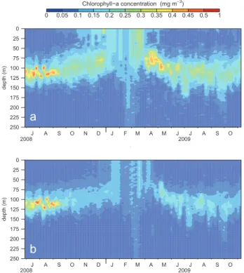
tion was achieved using MODIS 8-day data. The time se-ries of “satellite-corrected” profiles is presented in Fig. 7a. A well-marked seasonal cycle, consistent with previous ob-servations of Krom et al. (1992), is observed. This cy-cle presents a strong stratification of the water column in summer, characterized by a DCM between 100 and 125 m depth. During winter, Chl aC is quite constant through-out the mixed layer, which deepened to more than 250 m in February/March 2009. Chl aC values never exceeded 0.68 mg m−3.The maxima are observed at the DCM (summer 2008, spring 2009), in agreement with the well-known char-acteristics of the Mediterranean oligotrophic areas (Moutin and Raimbault, 2002).
For the sake of comparison, the modified Boss et al. (2008) method (see Sect. 4.2) was also applied (Fig. 7b). The two se-ries of profiles are consistent from July to September 2008, with Chl aC ranges between 0 and 0.65 mg m−3. Impor-tant differences are however observed for the rest of the pe-riod (from October 2008 to October 2009), when the “Boss-calibrated” Chl aCis lower (on average 0.15 mg m−3 differ-ence at DCM).
5 Discussion
Compared with HPLC references, “satellite-corrected” flu-orescence profiles are globally unbiased, presenting an r2 of about 67 % and a median error of about 31 %. These er-rors (Figs. 1, 3 and 4, Table 4) are certainly affected by the
Fig. 6. Comparison of the BATS monthly fluorescence-based Chl aCclimatology (black solid lines) to the HPLC-based climatology (black stars; see text and Appendix A for details about computation methods). For the fluorescence-based climatology, the retained shape (i.e. “stratified” or “mixed”) is indicated with its percentage of occurrence, and grey lines display all the “satellite-corrected” profiles representing the dominant shape.
uncertainty of satellite Chl aCmeasurements. Our analysis demonstrated that when the error of satellite Chl aCis lower than 35 % (i.e. the estimated averaged accuracy of ocean colour mission; McClain, 2009), our method performs better. However, several studies indicated that ocean colour Chl aC observations could have error greater than 35 %, in particu-lar over certain localised areas (e.g. the Mediterranean Sea; D’Ortenzio et al., 2002, the Antarctic or the Equatorial At-lantic; Gregg and Casey, 2004). In these situations, particu-lar attention should be dedicated to the interpretation of our “satellite-corrected” profiles.
The matchup procedure used to associate a satellite obser-vation with a fluorescence profile could also have an impact
on the final Chl aC profile. However, a narrower matchup protocol (i.e. 1-day) does not significantly enhance the per-formance (Table 1); although, conversely, it does decrease the number of available satellite observations, (cloud cover limits the satellite coverage in the match up box) and, there-fore, their statistical relevance.
Another potential source of error derives from the conver-sion of surface Chl aC into integrated Chl a content over the water column (Eq. (2), as obtained by regression anal-yses performed by Uitz et al., 2006). However, the use of vertically integrated contents to calculate the correction co-efficients, i.e. Eq. (4), does not change the method perfor-mance, when compared with HPLC estimations (Table 5).
date d e p th (m)
a
0 0.05 0.1 0.15 0.2 0.25 0.3 0.35 0.4 0.45 0.5 1 Chlorophyll−a concentration (mg m−3) 250 225 200 175 150 125 100 75 50 25 0 2008 2009 J A S O N D J F M A M J J A S O date d e p th (m)b
250 225 200 175 150 125 100 75 50 25 0 2008 2009 J A S O N D J F M A M J J A S OFig. 7. Time series of Chl aCdistribution estimated with a
fluorom-eter deployed on a profiling float in the Levantine Sea and processed with the present method (a) and with the Boss et al. (2008) method
(b).
We suppose that integrating over the 1.5Ze decreases the impact of the vertical variability of the Chl aC/fluorescence ratio on the final calculation of α. Additionally, using in-tegrated contents, the α calculation is less affected by the method of NPQ correction.
A possible alternative to Eq. (2) is the use of surface mea-surements, as proposed by Boss et al. (2008). In this case, however, the variability of the Chl aC/fluorescence relation-ship could have a larger impact on the final profile, as a pos-sible error in the surface data should propagate all along the water column. Moreover, for surface observations, the accu-racy of the NPQ correction (i.e. surface measurements are more affected by NPQ than deep values) and of the satellite estimations is likely crucial. In our data set tests, however, these effects seem minimized (Table 5) and we suppose that this is mainly due to the statistical significance of the regres-sion used to calculate αB (p-value = 2 × 10⁻⁷ for the
DY-FAMED subset). If the statistical relevance of the regression to calculate αBhad been low (e.g. few match-ups, important
satellite errors, regional biases), even profiles having a good satellite match-up would have been erroneously re-adjusted. The Boss et al. (2008) method therefore represents a pow-erful tool, and a valid alternative, to correct fluorescence pro-files and to produce vertical estimations of Chl aCconsistent with satellite data. Our method is merely an improvement of the Boss et al. (2008) method. The main
methodologi-cal differences between the two approaches seem to have a very weak impact on the final errors (Table 5), and the two methods appear equivalent from the point of view of the error analysis. However, the Boss et al. (2008) method was specif-ically developed to derive an accurate estimation of Chl aC from fluorescence measurements performed by a profiling float, which was (1) equipped with a unique fluorometer, (2) spanning a three-year period only, (3) floating in a limited, al-though vast, ocean region (western North Atlantic). For this reason, their method was based on a unique correction factor for all the series of profiles and, to match satellite observa-tions, they used only surface data.
Our objective has been to enhance the Boss et al. (2008) method so as to be able to process any fluorescence profile having a concurrent satellite observation (after 1997). Con-sequently, we decided to (1) generate a correction factor for each profile, (2) enlarge the temporal and spatial window of the satellite observations, to ensure a match-up, even in regions with low satellite coverage and (3) use 1.5Ze in-tegration depth instead of surface points only, to minimize the effect of the error propagation along the vertical scale in case of high vertical variability of the Chl aC/fluorescence ratio. We are confident that, with these characteristics, our method could be widely applied (e.g. to all fluorescence pro-files in the NODC database collected after 1997). Further-more, the corrected data set of fluorescence profiles could be used to generate a satellite/fluorescence blended product of the Chl aC.
The potential of this blended product is evident for the generation of a new type of climatology of Chl aC. Com-pared with a climatology generated with only discrete sam-ples (i.e. HPLC), the new fluorescence-based climatology ex-hibits some differences, mainly in the mixed layer and at the DCM (Fig. 6). The causes of these discrepancies must be as-cribed to methodological issues. In particular, climatologies based on HPLC discrete points generally require interpola-tions on the vertical scale, which could smooth the final mean profile (see Fig. 6). Additionally, averaging mixed and strati-fied profiles generates atypical shapes (see winter months of the HPLC-based climatology at BATS, Fig. 6), which have no correspondence with the initial data set, but are pure arte-facts of the mean procedure. In the new fluorescence-based climatology (Fig. 6), the dominant shape (i.e. stratified or mixed) appears more clearly and the proposed method to calculate the climatological profile results in marked DCM peaks, as generally expected.
The merging method proposed here has also been ap-plied to a profiling float fluorometer, and the obtained re-sults were compared with those derived from the method of Boss et al. (2008), which was specifically developed for pro-filing float data. The application of the two procedures on a single set of fluorescence profiles leads to different results (Fig. 7). At the present stage, it is impossible to definitely assess which method is closest to the truth. However, both the methods are consistent, by definition, with the concurrent
satellite estimations. In other words, the profiling float obser-vations could be easily merged with satellite ocean colour maps, to finally generate a unique 3-D picture of the Chl aC field. The use of this 3-D picture of Chl aCcould improve the operational simulations of oceanic ecosystems, in partic-ular in an assimilation scheme (Brasseur et al., 2009). In this context, our method appears more promising than the Boss et al. (2008) procedure, which rather requires the utilisation of all the fluorescence profiles achieved during the whole life-time of the float to determine correction coefficients, and thus cannot be applied in real-time.
6 Conclusions
We have presented a method to merge fluorescence profiles and satellite ocean colour observations, which allows uni-forming the existing Chl aCestimations derived from fluo-rescence observations. Fluofluo-rescence profiles, obtained from a range of fluorometers and factory calibrations and under various trophic and environmental conditions, were corrected with a unique and stable reference provided by ocean colour satellites. Consequently, for the first time, the huge data set of fluorescence profiles collected during the last 15 yr could be inter-compared. Moreover, the corrected fluorescence pro-files are consistent with satellite observations; their integra-tion and merging with other data sources should be strongly facilitated.
The limits of the present method are essentially deter-mined by the limits of the data sets used (i.e. fluorescence and satellite observations). If no satellite match-ups are available, a merging procedure cannot be performed. Consequently, all fluorescence profiles performed before 1997 (date of launch-ing of the SeaWiFS sensor), as well as profiles achieved in high latitudes, cannot be merged with satellite data. Biases are also induced by the error of satellite ocean colour, which represents the first source of error of our method. However, the error estimated by comparing “satellite-corrected” flu-orescence profiles with HPLC estimations is only slightly higher than the error estimated for the ocean colour satel-lite observations. In addition, packaging effect constitutes another limit of the method, because vertical a∗ variability was not resolved in the method. Strictly speaking, the pro-posed method is not a calibration procedure, which should imply a more accurate evaluation of the sensor responses. In our approach, fluorescence profiles are only corrected and re-adjusted to be consistent with satellite estimations. Neverthe-less, the resulting corrected profiles show lower errors than the initial fluorescence profiles, when compared with HPLC estimations.
Although we accept that the merging method presented here cannot substitute, in terms of accuracy, the calibrations derived from laboratory analyses to determine Chl aC, it does, nevertheless, present specific advantages that could be particularly adapted for specific applications. We presented
here two examples: the improvement of the Chl aC clima-tology and the treatment of fluorescence data measured by a profiling float. These two applications will probably con-verge in the future: at the present time, the only clima-tology available (Conkright et al., 2002) is based on dis-crete bottle data and suffers from (1) a critical lack of data and (2) a really poor vertical resolution. Integrating existing “satellite-corrected” fluorescence profiles in Chl aC clima-tologies should help in filling these gaps. Moreover, the high flux of fluorescence data provided by the increased number of profiling floats will definitively reinforce our capacity for describing, climatologically and in real time, the Chl aCfield. In this framework, our approach could be considered one of the steps for a future quality control system for a network of profiling floats. However, it should be used only when other methods fail or are inapplicable, to prevent any redundant in-formation or circular exercise if a validation of satellite ocean colour products is attempted with the profiling floats obser-vations.
Appendix A
Procedure to generate the new, fluorescence-based, Chl aCclimatology
1. All the fluorescence profiles available for a given month were sorted into two categories: stratified and mixed with respect to the Zm/Zeratio. If Zm/Ze>1, the pro-file is associated with the mixed category; otherwise, it is associated with the stratified category.
2. On one hand, the climatological profile representing the stratified category was computed as follows: (a) on each stratified profile, the DCM was identified as the ab-solute maximum on the vertical scale; (b) the profile depths were normalized by the depth of the DCM; (c) all the depth-normalized profiles were then averaged, for each unity of the dimensionless vertical scale; (d) the resulting mean profile was finally reconverted to a metric scale, using a multiplicative factor obtained by averaging the DCM depths of all the profiles. On the other hand, the climatological profile corresponding to the mixed category was computed in a similar way as the climatological stratified profile except that the DCM depth used for normalization was replaced by the mixed layer depth.
3. Finally, only the climatological profile corresponding to the more frequent category (stratified or mixed) was re-tained to represent the monthly climatological Chl a dis-tribution.
Acknowledgements. The authors would like to thank all the staff
of the DYFAMED observation service and of the BATS and HOT programs for the periodic measurements of oceanographic variables, and for the free distribution of data online. The US NASA space agency is thanked for the easy access to SeaWiFS and MODIS data. The authors are also grateful to Louis Prieur and Alexandre Mignot, for constructive comments and suggestions, to Jos´ephine Ras for reviewing the manuscript and to Emmanuel Boss (Univ. of Maine) who kindly provided details about his method. This paper is a contribution to the PABIM (Plateformes Autonomes Biog´eochimiques: Instrumentation et Mesures) project funded by the Groupe Mission Mercator Coriolis (GMMC), to the PABO (Plateformes Autonomes and Biog´eochimie Oc´eanique) project funded by Agence Nationale de la Recherche (ANR) and to the remOcean (REMotely sensed biogeochemical cycles in the OCEAN) project, funded by the Grant agreement No. 246777. Edited by: E. Boss
The publication of this article is financed by CNRS-INSU.
References
Althuis, I. A., Gieskes, W. W. C., Villerius, L., and Colijn, F.: In-terpretation of fluorometric chlorophyll registrations with Algal pigment analysis along a ferry transect in the Southern North Sea, Neth. J. Sea Res., 33, 37–46, 1994.
Bailey, S. and Werdell, P.: A multi-sensor approach for the on-orbit validation of ocean color satellite data products, Remote Sens. Environ., 102, 12–23, doi:10.1016/j.rse.2006.01.015, 2006. Behrenfeld, M. J. and Boss, E.: Beam attenuation and
chlorophyll concentration as alternative optical indices of phytoplankton biomass, J. Mar. Res., 64, 431–451, doi:10.1357/002224006778189563, 2006.
Bosc, E., Bricaud, A., and Antoine, D.: Seasonal and inter-annual variability in algal biomass and primary production in the Mediterranean Sea, as derived from 4 years of Sea-WiFS observations, Global Biogeochem. Cy., 18, GB1005, doi:10.1029/2003GB002034, 2004.
Boss, E., Collier, R., Larson, G., Fennel, K., and Pegau, W.: Measurements of spectral optical properties and their rela-tion to biogeochemical variables and processes in Crater Lake, Crater Lake National Park, OR, Hydrobiologia, 574, 149–159, doi:10.1007/s10750-006-2609-3, 2007.
Boss, E., Swift, D., Taylor, L., Brickley, P., Zaneveld, R., Riser, S., Perry, M., and Strutton, P.: Observations of pigment and particle distributions in the western North Atlantic from an autonomous float and ocean color satellite, Limnol. Oceanogr., 53, 2112– 2122, doi:10.4319/lo.2008.53.5 part 2.2112, 2008.
Boyer, T., Antonov, J., Baranova, O., Garcia, H., Johnson, D., Lo-carnini, R., Mishonov, A., O’Brien, T., Seidov, D., Smolyar, I.,
and Zweng, M.: World Ocean Database 2009, edited by: Levitus, S., NOAA Atlas NESDIS 66U.S. Gov. Printing Office, Wash., DC, 216 pp., DVDs, 2009.
de Boyer Montegut, C., Madec, G., Fischer, A., Lazar, A., and Iu-dicone, D.: Mixed layer depth over the global ocean: An exami-nation of profile data and a profile-based climatology, J. Geophy. Res.-Oceans, 109, C12003, doi:10.1029/2004JC002378, 2004. Brasseur, P., Gruber, N., Barciela, R., Brander, K., Doron, M., El
Moussaoui, A., Hobday, A., Huret, M., Kremeur, A., Lehodey, P., Matear, R., Moulin, C., Muturgudde, R., Senina, I., and Svend-sen, E.: Integrating Biogeochemistry and Ecology Into Ocean Data Assimilation Systems, Oceanography, 22, 206–215, 2009. Campbell, J. W.: The lognormal distribution as a model for
bio-optical variability in the sea, J. Geophys. Res., 100, 13237– 13254, doi:199510.1029/95JC00458, 1995.
Cetinic, I., Toro-Farmer, G., Ragan, M., Oberg, C., and Jones, B.: Calibration procedure for Slocum glider deployed optical instru-ments, Optics Express, 17, 15420–15430, 2009.
Claustre, H., Morel, A., Babin, M., Cailliau, C., Marie, D., Marty, J.-C., Tailliez, D. and Vaulot, D.: Variability in particle attenua-tion and chlorophyll fluorescence in the tropical Pacific: scales, patterns, and biogeochemical implications, J. Geophys. Res., 104, 3401–3422, 1999.
Claustre, H., Antoine, D., Boehme, L., Boss, E., D’Ortenzio, F., Fanton D’Andon, O., Guinet, C., Gruber, N., Handegard, N. O., Hood, M., Johnson, K., Lampitt, R., LeTraon, P.-Y., Lequ´er´e, C., Lewis, M., Perry, M.-J., Platt, T., Roemmich, D., Testor, P., Sathyendranath, S., Send, U., and Yoder, J.: Guidelines To-wards an Integrated Ocean Observation System for Ecosystems and Biogeochemical Cycles, in: Proceedings of OceanObs’09: Sustained Ocean Observations and Information for Society (Vol. 2), Venice, Italy, 21–25 September 2009, edited by: Hall, J., Harrison, D. E., and Stammer, D., ESA Publication WPP-306, doi:10.5270/OceanObs09.pp.14, 2010.
Cleveland, J. S. and Perry, M. J.: Quantum yield, relative specific absorption and fluorescence in nitrogen-limited Chaetoceros gra-cilis, Mar. Biol., 94, 489–497, 1987.
Conkright, M., O’Brien, T., Stephens, K., Locarnini, R., Garcia, H., Boyer, T., and Antonov, J.: World Ocean Atlas 2001, Volume 6: Chlorophyll, edited by: Levitus, S., NOAA Atlas NESDIS 54, US Governement Printing Office, Wash., DC, 46 pp., 2002. Cullen, J.: The Deep Chlorophyll Maximum – Comparing Vertical
Profiles of Chlorophyll-A, Can. J. Fish. Aquat. Sci., 39, 791–803, 1982.
Cullen, J. and Lewis, M.: Biological processes and optical measure-ments near the sea surface: some issues relevant to remote sens-ing, J. Geophy. Res-Oceans, 100, 13255–13266, 1995.
Davis, R. F., Moore, C. C., Zaneveld, J. R. V., and Napp, J. M.: Reducing the effects of fouling on chlorophyll estimates derived from long-term deployments of optical instruments, J. Geophys. Res., 102, 5851–5855, doi:199710.1029/96JC02430, 1997. D’Ortenzio, F., Marullo, S., Ragni, M., Ribera d’Alcal`a, M.,
and Santoleri, R.: Validation of empirical SeaWiFS algorithms for chlorophyll-a retrieval in the Mediterranean Sea: A case study for oligotrophic seas, Remote Sens. Environ., 82, 79–94, doi:16/S0034-4257(02)00026-3, 2002.
D’Ortenzio, F., Iudicone, D., Montegut, C., Testor, P., Antoine, D., Marullo, S., Santoleri, R., and Madec, G.: Seasonal vari-ability of the mixed layer depth in the Mediterranean Sea as
derived from in situ profiles, Geophys. Res. Lett., 32, L12605, doi:10.1029/2005GL022463, 2005.
D’Ortenzio, F., Thierry, V., Eldin, G., Claustre, H., Testor, P., Coatanoan, C., Tedetti, M., Guinet, C., Poteau, A., Prieur, L., Lefevre, D., Bourin, F., Carval, T., Goutx, M., Garc¸on, V., Thouron, D., Lacombe, M., Lherminier, P., Loisel, H., Mortier, L., and Antoine, D.: White Book on Oceanic Autonomous Plat-forms for Biogeochemical Studies: Instrumentation and Mea-sure (PABIM) version 1.3, available at: http://www.obs-vlfr.fr/ OAO/file/PABIM white book version1.3.pdf (last access: 2012), 2010.
Falkowski, P. and Kiefer, D. A.: Chlorophyll a fluorescence in phy-toplankton: relationship to photosynthesis and biomass, J. Plank-ton Res., 7, 715–731, 1985.
Feldman, G., Kuring, N., Ng, C., Esaias, W., McClain, C., El-rod, J., Maynard, N., and Endres, D.: Ocean color: Avail-ability of the global data set, Eos Trans. AGU, 70, 634, doi:10.1029/89EO00184, 1989.
Gieskes, W. W. and Kraay, G. W.: Unknown Chlorophyll a deriva-tives in the North Sea and the Tropical Atlantic ocean revealed by HPLC analysis, Limnol. Oceanogr., 28, 757–766, 1983. Gregg, W. W. and Conkright, M.: Global seasonal climatologies
of ocean chlorophyll: Blending in situ and satellite data for the Coastal Zone Color Scanner era, J. Geophy. Res.-Oceans, 106, 2499–2515, 2001.
Gregg, W. W. and Casey, N. W.: Global and regional evaluation of the SeaWiFS chlorophyll data set, Remote Sens. Environ., 93, 463–479, doi:10.1016/j.rse.2003.12.012, 2004.
Holm-Hansen, O., Lorenzen, C. J., Holmes, R. W., and Strickland, J. D. H.: Fluorometric Determination of Chlorophyll, Ices J. Mar. Sci., 30, 3–15, doi:10.1093/icesjms/30.1.3, 1965.
Hooker, S. B., Van Heukelem, L., Thomas, C. S., Claustre, H., Ras, J., Sch¨ulter, L., Clementson, L., Van der Linde, L., Eker-Develi, E., Berthon J.-F., Barlow, R., Sessions, H., Ismail, H., and Perl, J.: The third SeaWiFS HPLC Analysis Round-Robin Experiment (SeaHARRE-3), NASA technical Memorandum 2009-215849, Greenbelt: NASA Goddard Space Flight Center, 2009.
Karl, D. M. and Lukas, R.: The Hawaii Ocean Time-series (HOT) program: Background, rationale and field implementation, Deep-Sea Res. Pt. II, 43, 129–156, doi:16/0967-0645(96)00005-7, 1996.
Kiefer, D. A.: Fluorescence properties of natural phytoplankton populations, Mar. Biol., 22, 263–269, 1973.
Kolber, Z. and Falkowski, P. G.: Use of Active Fluorescence to Esti-mate Phytoplankton Photosynthesis in Situ, Limnol. Oceanogr., 38, 1646–1665, 1993.
Krom, M., Brenner, S., Kress, N., Neori, A., and Gorgon, L.: Nutri-ent Dynamics and New Production in a Warm-Core Eddy from the Eastern Mediterranean-Sea, Deep-Sea Res., 39, 467–480, 1992.
Loftus, M. and Seliger, H.: Some Limitation of the In Vivo Fluores-cence Technique, Chesapeake Science, 16, 79–92, 1975. Lorenzen, C. J.: A method for the continuous measurement of in
vivo chlorophyll concentration, Deep-Sea Res., 13, 223–227, 1966.
Lorenzen, C. J.: Determination of Chlorophyll and Pheo-Pigments: Spectrophotometric Equations, Limnol. Oceanogr., 12, 343–346, 1967.
Mantoura, R. F. C. and Llewellyn, C. A.: The rapid determi-nation of algal chlorophyll and carotenoid pigments and their breakdown products in natural waters by reverse-phase high-performance liquid chromatography, Anal. Chim. Acta, 151, 297–314, doi:10.1016/S0003-2670(00)80092-6, 1983.
Marty, J.-C., Chiav´erini, J., Pizay, M.-D. and Avril, B.: Seasonal and interannual dynamics of nutrients and phytoplankton pig-ments in the western Mediterranean Sea at the DYFAMED time-series station (1991–1999), Deep-Sea Res. Pt. II, 49, 1965–1985, doi:16/S0967-0645(02)00022-X, 2002.
McClain, C. R.: A Decade of Satellite Ocean Color Observations, Annual Rev. Mar. Sci., 1, 19–42, doi:10.1146/annurev.marine.010908.163650, 2009.
McClain, C., Cleave, M., Feldman, G., Gregg, W., Hooker, S., and Kuring, N.: Science quality SeaWiFS data for global biosphere research, Sea Technol., 39, 10–16, 1998.
Michaels, A. F. and Knap, A. H.: Overview of the U.S. JGOFS Bermuda Atlantic Time-series Study and the Hydrostation S program, Deep-Sea Res. Pt. II, 43, 157–198, doi:16/0967-0645(96)00004-5, 1996.
Mignot, A., Claustre, H., D’Ortenzio, F., Xing, X., Poteau, A., and Ras, J.: From the shape of the vertical profile of in vivo fluores-cence to Chlorophyll-a concentration, Biogeosciences, 8, 2391– 2406, doi:10.5194/bg-8-2391-2011, 2011.
Moore, T. S., Campbell, J. W., and Dowell, M. D.: A class-based approach to characterizing and mapping the uncertainty of the MODIS ocean chlorophyll product, Remote Sens. Environ., 113, 2424–2430, doi:10.1016/j.rse.2009.07.016, 2009.
Morel, A.: Optical modeling of the upper ocean in relation to its biogenous matter content (case-I waters), J. Geophy. Res-Oceans, 93, 10749–10768, 1988.
Morel, A. and Berthon, J.: Surface pigments, algal biomass profiles, and potential production of the euphotic Layer – Relationships reinvestigated in view of remote-sensing applications, Limnol. Oceanogr., 34, 1545–1562, 1989.
Morel, A. and Bricaud, A.: Theoretical results concerning light absorption in a discrete medium, and application to specific absorption of phytoplankton, Deep-Sea Res., 28, 1375–1393, doi:10.1016/0198-0149(81)90039-X, 1981.
Morel, A. and Maritorena, S.: Bio-optical properties of oceanic wa-ters: A reappraisal, J. Geophy. Res.-Oceans, 106, 7163–7180, 2001.
Moutin, T. and Raimbault, P.: Primary production, carbon export and nutrients availability in western and eastern Mediterranean Sea in early summer 1996 (MINOS cruise), J. Marine Syst., 33– 34, 273–288, doi:10.1016/S0924-7963(02)00062-3, 2002. M¨uller, P., Li, X.-P., and Niyogi, K. K.: Non-Photochemical
Quenching. A Response to Excess Light Energy, Plant Physiol., 125, 1558–1566, doi:10.1104/pp.125.4.1558, 2001.
Ras, J., Claustre, H., and Uitz, J.: Spatial variability of phytoplank-ton pigment distributions in the Subtropical South Pacific Ocean: comparison between in situ and predicted data, Biogeosciences, 5, 353–369, doi:10.5194/bg-5-353-2008, 2008.
Rochford, P., Kara, A., Wallcraft, A. and Arnone, R.: Importance of solar subsurface heating in ocean general circulation models, J. Geophy. Res.-Oceans, 106, 30923–30938, 2001.
Sackmann, B. S., Perry, M. J., and Eriksen, C. C.: Seaglider ob-servations of variability in daytime fluorescence quenching of chlorophyll-a in Northeastern Pacific coastal waters,
Biogeo-sciences Discuss., 5, 2839–2865, doi:10.5194/bgd-5-2839-2008, 2008.
Sharples, J., Moore, C. M., Rippeth, T. P., Holligan, P. M., Hydes, D. J., Fisher, N. R., and Simpson, J. H.: Phytoplankton Distribution and Survival in the Thermocline, Limnol. Oceanogr., 46, 486– 496, 2001.
Steinberg, D., Carlson, C., Bates, N., Johnson, R., Michaels, A. and Knap, A.: Overview of the US JGOFS Bermuda Atlantic Time-series Study (BATS): a decade-scale look at ocean biology and biogeochemistry, Deep-Sea Res. Pt. II, 48, 1405–1447, 2001. Strass, V.: On the calibration of large-scale fluorometric chlorophyll
measurements from towed undulating vehicles, Deep-Sea Res., 37, 525–540, doi:10.1016/0198-0149(90)90023-O, 1990. Strickland, J. D. H.: Production of organic matter in primary stages
of the marine food chain, in Chemical Oceanography, edited by: Riley, J. P. and Skirrow, G., Academic Press, London, 477–610, 1965.
Strickland, J. D. H.: Continuous measurement of in vivo chloro-phyll; a precautionary note, Deep-Sea Res., 15, 225–227, 1968. Uitz, J., Claustre, H., Morel, A., and Hooker, S.: Vertical
distribu-tion of phytoplankton communities in open ocean: An assess-ment based on surface chlorophyll, J. Geophy. Res.-Oceans, 111, C08005, doi:10.1029/2005JC003207, 2006.
Xing, X., Morel, A., Claustre, H., Antoine, D., D’Ortenzio, F., Poteau, A. and Mignot, A.: Combined processing and mutual in-terpretation of radiometry and fluorimetry from autonomous pro-filing Bio-Argo floats: Chlorophyll a retrieval, J. Geophys. Res., 116, C06020, doi:10.1029/2010JC006899, 2011.
Xing, X., Claustre, H., Blain, S., D’Ortenzio, F., Antoine, D., Ras, J., and Guinet, C.: Quenching correction for in vivo chlorophyll fluorescence measured by instrumented elephant seals in the Ker-guelen region (Southern Ocean), Limnol. Oceanogr.-Meth., in press, 2012.