HAL Id: hal-02435793
https://hal.archives-ouvertes.fr/hal-02435793
Submitted on 11 Jan 2020
HAL is a multi-disciplinary open access
archive for the deposit and dissemination of
sci-entific research documents, whether they are
pub-L’archive ouverte pluridisciplinaire HAL, est
destinée au dépôt et à la diffusion de documents
scientifiques de niveau recherche, publiés ou non,
An Optimal Algorithm To Recognize Robinsonian
Dissimilarities
Pascal Préa, Dominique Fortin
To cite this version:
Pascal Préa, Dominique Fortin. An Optimal Algorithm To Recognize Robinsonian Dissimilarities.
Journal of Classification, Springer Verlag, 2014. �hal-02435793�
An Optimal Algorithm To Recognize Robinsonian Dissimilarities
Pascal Pr´
ea
∗†LIF, Laboratoire d’Informatique Fondamentale de Marseille, CNRS UMR 7279 ´
Ecole Centrale Marseille
Technopˆole de Chˆateau-Gombert, 38, rue Joliot Curie, 13451 Marseille C´edex 20, France
Dominique Fortin
INRIA
Domaine de Voluceau, Rocquencourt, B.P. 105, 78153 Le Chesnay C´edex, France
Abstract
A dissimilarity D on a finite set S is said to be Robinsonian if S can be totally ordered in such a way that, for every i < j < k, D(i, j) ≤ D(i, k) and D(j, k) ≤ D(i, k). Intuitively, D is Robinsonian if S can be represented by points on a line. Recognizing Robinsonian dissimilarities has many applications in se-riation and classification. In this paper, we present an optimal O(n2
) algorithm to recognize Robinsonian dissimilarities, where n is the cardinal of S. Our result improves the already known algorithms.
Key Words
Robinsonian Dissimilarities; Classification, Seriation; Interval Graphs, PQ-Trees, Consecutive One’s Property, Partition Refinement.
1
Introduction
A dissimilarity on a finite set S is a symmetric function D : S × S → IR+ such that D(i, j) = 0 if i = j.
Dissimilarities can be seen as a generalization of distances. A dissimilarity on an n-set S can be represented by a symmetric n × n matrix on IR+with a null diagonal, and we shall identify dissimilarities and symmetric
non negative matrices with null diagonal. An n × n matrix (or dissimilarity) D on a set S is said to be Robinsonian if S can be linearly sorted in such a way that, for every i < j < k, D(i, j) ≤ D(i, k) and D(j, k) ≤ D(i, k) (Robinson 1951). Such an order is called a compatible order or a compatible permutation. If D is Robinsonian and S is sorted along a compatible order, then all the rows and columns of D (considered as a matrix) are non-decreasing when going from the diagonal.
Robinsonian dissimilarities first appeared as a tool to solve problems in seriation of archeological deposits (Robinson 1951). Given a set of archeological deposits, archeologists often make the following hypothesis: the further in time are the deposits, the farther they are from a stylistic point of view; that is to say that, when we measure the stylistic difference between deposits, we get a Robinsonian dissimilarity, and the chronological ordering (which is looked for) is one of the compatible orderings (see Petrie 1899, Kendall 1969). Similar problems arise in musicology (see Halperin 1994), matrix visualisation (see Caraux and Pinloche 2005, Chen and all 2004), philology (see Boneva 1980), hypertext analysis (see Berry and all 1996), ecology (see Mikl´os and all 2005), DNA sequencing (see Benzer 1962, Mirkin and Rodin 1984) . . . Actually, Robinsonian
∗Corresponding author.
dissimilarities appear when data has a underlying linear total ordering and they play a prominent role in seriation.
In addition, Robinsonian dissimilarities are a generalization of ultrametrics (a distance D on a set S is an ultrametric if ∀x, y, z ∈ S, D(x, y) ≥ max(D(x, z), D(y, z))) which are in one-to-one correspondence with hierarchies (see Bart´elemy and Gu´enoche 1991, Critchley and Fichet 1994). Similarly, Robinson dissimi-larities are in one-to-one correspondence with a generalization of hierarchies, namely the indexed pseudo hierarchies, also called pyramids (see Durand and Fichet 1988 and Diday 1986). A pseudo-hierarchy on a set S is a subset H of P(S), whose elements are called classes and such that:
• S ∈ H.
• ∀x ∈ S, {x} ∈ H.
• ∀h, h′∈ H, (h ∩ h′= ∅) or (h ∩ h′ ∈ H).
• There exists an order ≤H on S such that, when S is sorted along ≤H, every class is an interval.
A (weak) index on a pseudo hierarchy H is a function i : H → IR+ such that:
• ∀x ∈ S, i({x}) = 0.
• ∀h, h′∈ H, h ⊂ h′ =⇒ i(h) ≤ i(h′).
• ∀h, h′∈ H, h ! h′, i(h) = i(h′) =⇒ h′ =!{h” ∈ H : h ! h”}.
Given an indexed pseudo hierarchy (H, i), the dissimilarity D defined by D(x, y) is the index of the smallest class containing x and y is Robinsonian. Conversely, given a Robinsonian dissimilarity D, it is possible to construct a pseudo-hierarchy from the set BD= {B(x, λ), x ∈ S, λ ∈ IR+}, where B(x, λ) = {y ∈ S, D(x, y) ≤
λ}. More precisely, if D is a Robinsonian dissimilarity on a finite set S, then {B(x, D(x, y)) ∩ B(y, D(x, y)) : x, y ∈ S} is a pseudo hierarchy on S. This one-to-one correspondence makes Robinsonian dissimilarities have many applications in classification and data analysis (see Durand and Fichet 1988 ,Critchley and Fichet 1994, Strehl and Ghosh 2003).
From a graph theoretical point of view, these dissimilarities are in relation with interval hypergraphs (see Fulkerson and Gross 1965). An interval hypergraph is an hypergraph (i.e. a vertex set V with a hyperedge set E, each hyperedge being a subset of V ) such that the vertex set can be ordered in such a way that every hyperedge is an interval; given a dissimilarity D on a set S, (S, BD) is an interval hypergraph if and only if
D is Robinsonian.
The first polynomial algorithm to recognize Robinsonian dissimilarities was given in Mirkin and Rodin (1984). This algorithm is based on the relation between interval hypergraphs and Robinsonian dissimilarities; it runs in O(n4) time and O(n3) space. Chepoi and Fichet (1997) and Seston (2008a) gave O(n3) time and
O(n2) space algorithms to recognize Robinsonian dissimilarities; these algorithms consider the values of D
in decreasing order. The first of these algorithms uses the divide-and-conquer paradigm, and the second one constructs paths in threshold graphs of D. Seston (2008b) improved the second algorithm to O(n2log n).
Optimal L∞-fitting of a dissimilarity by a Robinsonian dissimilarity is a NP-hard problem (see Barth´elemy
and Brucker 2003 and Chepoi and all 2009). So, there is no efficient exact algorithms for this problem, and one has to use heuristics like Brusco (2002) and Hubert (1974), or an approximation algorithm like Chepoi and Seston (2011).
In this paper, we present a new algorithm to recognize Robinsonian dissimilarities, based on interval graphs (see Golumbic 1980). Our algorithm runs in O(n2) time. Since the recognition of Robinsonian
matrices needs at least to check all the elements of the matrix, our algorithm is optimal.
In Section 2, we establish some links between Robinsonian dissimilarities and interval graphs and give a sketch of our algorithm. In Sections 3, we give some sub-routines which are needed by our algorithm. In Section 4, we give a precise description of our algorithm. In Section 5, we show, on an example, how our algorithm runs. In Section 6, we mention some other applications of our algorithm.
The crucial idea of our algorithm is to consider the values D(x, y) in increasing order. So, we first consider small values of D from which we get local necessary conditions on the permutations compatible with Robinson property. Although local, these informations are quite accurate: we get subsets of S such that, if D is Robinsonian, then for every compatible permutation σ, these subsets are intervals of S when S
is sorted along σ.
Then we retrieve the relative locations of these intervals thanks to large values of D (opposite to increasing threshold); however, we do not have to consider all the points of S: since the informations on the intervals are accurate, we just have to keep one or two representatives for each interval and recursively apply our algorithm on the set of representatives. This set of representatives remains small enough to guarantee that the recursion does not change the overall complexity. The major achievement over previous algorithms relies on this parsimonious shrinking of points of S.
For the sake of simplicity, our algorithm does not systematically test if D is Robinsonian or not. So, after the recursive calls, we are in one of the following two cases:
• If D is Robinsonian, then we have the set of the compatible permutations. • If D is not Robinsonian, then we have an arbitrary set of permutations.
In order to distinguish between these two cases, we just have to take one (arbitrary) permutation of the returned set and test if it is a compatible permutation or not.
2
Robinsonian dissimilarities and interval graphs
The main goal of this section is to give some links between Robinsonian dissimilarities and interval graphs. This is a kind of folklore and, for instance, such results can be found in Mirkin and Rodin (1984). All sets and graphs considered in this paper are finite.
A graph G = (V, E) is an interval graph if G is the intersection graph of a family of intervals on the real line, i.e. if there exists a family I of intervals such that V = {xi, i ∈ I} and {xi, xj} ∈ E ⇐⇒ i ∩ j ̸= ∅
(see Golumbic 1980). It is well known (see Gilmore and Hoffman 1964) that graph G is an interval graph if and only if its maximal cliques can be linearly ordered in such a way that if c1< c2< c3, i ∈ c1 and i ∈ c3,
then i ∈ c2. Equivalently, the vertex-clique incidence matrix of G has the Consecutive One’s Property: if the
rows are indexed by the vertices and the columns are indexed by the maximal cliques, it is possible to sort the columns in such a way that, on every row, the 1’s appear consecutively. The set of all the compatible orders for a dissimilarity can be represented by a PQ-tree (see Booth 1975, Lueker 1975 and Booth and Lueker 1976). A PQ-tree T on a set S is a tree that represents a set of permutations on S. The leaves of T are the elements of S, and the nodes of T are of two types : the P-nodes and the Q-nodes. We use the general convention of writing that is to represent P-nodes by circles, and Q-nodes by rectangles. On a P-node, one can apply any permutation of its children (equivalently, its children are not ordered). The children of a Q-node are ordered, and the only permutation we can apply on them is to reverse the order. For instance, the PQ-tree of figure 1 represents the set of permutations {(1,2,3,4,5), (1,3,2,4,5), (2,1,3,4,5), (2,3,1,4,5), (3,1,2,4,5), (3,2,1,4,5), (5,4,1,2,3), (5,4,1,3,2), (5,4,2,1,3), (5,4,2,3,1), (5,4,3,1,2), (5,4,3,2,1)}. ✐ !! ❅❅ 1 2 3 4 5 Figure 1: A PQ-tree
For a node α of a PQ-tree T , we denote by T (α) the subtree of T with root α and by Sα the set of the
leaves of T (α). We will say that a node is basic if all its children are leaves. Claim 1. For any permutation represented by T , Sα is an interval of S.
Let D be a dissimilarity on an n-set S. For every x in S and k in [0, . . . , n], we define the sets Γk(x) by
setting:
• Γk(x) = {y ∈ S, ∀z ∈ S \ Γk−1(x), D(x, y) ≤ D(x, z)}.
Equivalently,
• Γ0(x) = ∆0(x) = {x},
• ∆k(x) = {y ∈ S \ Γk−1(x), ∀z ∈ S \ Γk−1(x), D(x, y) ≤ D(x, z)},
• Γk(x) = Γk−1(x) ∪ ∆k(x).
The sets ∆k(x) are spheres with center x, and the sets Γk(x) are balls with center x. Intuitively speaking,
∆1(x) contains the elements of S closest from x, the sphere made of its “inner circle” of neighbors, ∆2(x)
contains the “second circle” of neighbors,. . . For all i, Γk(x) is the unions of the k first ∆i(x).
Claim 2. If D is Robinsonian and S is sorted along a compatible order, then the sets Γk(x) are intervals.
We will call these sets Γ-intervals.
For every l in [0, . . . , n], we define the intersection graph Gl= (Vl, El), where:
• Vl= {Γk(x), x ∈ S, 0 ≤ k ≤ l}
• El= {{vi, vj}, vi∩ vj ̸= ∅}
On Figure 2, one can see that two different dissimilarities on three points a, b, c yield two different graphs G1, although, for these four dissimilarities, the intersection graphs of {Γ1(x)} or {Γ2(x)} are K3, and the
intersection graph of {Γ1(x)} ∪ {Γ2(x)} is K6. a b c a b c 0 2 3 0 1 0 .−→ " Γ1(c) " Γ1(a) " Γ1(b) "Γ0(c) = {c} "Γ0(a) = {a} "Γ0(b) = {b} ✁✁ ❆ ❆ ✏✏✏✏ ✏✏ &&& &&& ❛❛ ❛❛❛ a b c a b c 0 2 2 0 1 0 .−→ " Γ1(c) " Γ1(a) " Γ1(b) "Γ0(c) "Γ0(a) "Γ0(b) ✁✁ ❆ ❆ ✏✏✏✏ ✏✏ &&& &&& ◗ ◗ ◗ ◗ ◗ ◗ ❛❛ ❛❛❛ a b c a b c 0 1 3 0 1 0 .−→ " Γ1(c) " Γ1(a) " Γ1(b) "Γ0(c) "Γ0(a) "Γ0(b) ✁✁ ❆ ❆ ✏✏✏✏ ✏✏ &&& &&& ✦✦✦✦ ✦ ❛❛ ❛❛❛ a b c a b c 0 1 1 0 1 0 .−→ " Γ1(c) " Γ1(a) " Γ1(b) "Γ0(c) "Γ0(a) "Γ0(b) ✁✁ ❆ ❆ ✏✏✏✏ ✏✏ ✑✑ ✑✑ ✑✑ &&& &&& ◗ ◗ ◗ ◗ ◗ ◗ ✦✦✦✦ ✦ ❛❛ ❛❛❛
Figure 2: The graphs G1for the four dissimilarities on three points
The graphs Gl do not contain all the information on D. Let x and y be two elements of S. We say that
Property 1. If D is Robinsonian, then, for any l in [0,. . . ,n], Glis an interval graph. In addition, the set
of the permutations compatible with D is a subset of the set represented by the PQ-tree of Gl.
Proof. Follows from Claim 2.
It is clear that, if I is a set of horizontal intervals, then the maximal cliques of the intersection graph of I corresponds to vertical lines (see Figure 3). For the graphs Gl, we have the more precise property 2.
Figure 3: Maximal cliques of an interval graph
Property 2. If D is Robinsonian, then for any l in [0, . . . , n], the maximal cliques of Gl are in one-to-one
correspondence with the points of S.
Proof. Let C = {v1, . . . vp} be a maximal clique of Gl. By Claim 2, each viis an interval, so v1∩ . . . ∩ vp ̸= ∅.
Suppose that v1∩ . . . ∩ vp = {x1, . . . , xq}, with q > 1. The set Γ0(x1) is not in C (it does not contain xq),
but it intersects all the elements of C. So C ∪ {Γ0(x1)} is also a clique, which is in contradiction with the
maximality of C. So each maximal clique contains one (and only one) set Γ0(x).
Conversely, each element x of S corresponds to one maximal clique, namely the clique which contains Γ0(x).
Property 3. For any k in [0, . . . , n − 1] and any x in S, if Γk(x) = Γk+1(x), then Γk(x) = S.
Proof. If Γk(x) = Γk+1(x), then ∆k+1(x) = ∅, and so S \ Γk(x) = ∅
Corollary 1. For any k in [0, . . . , n − 1] and any x in S, |Γk(x)| > k.
Proof. Since |Γ0(x)| = 1, if for every i < k, |Γi+1(x)| > |Γi(x)|, then |Γk(x)| > k. Otherwise, by Property 3,
|Γk(x)| = n > k.
Theorem 1. (Mirkin and Rodin 1984 p.62) D is Robinsonian if and only if Gn is an interval graph. In this
case, the PQ-tree of Gn represents the set of the permutations compatible with D.
Proof. By Property 1, if D is Robinsonian, then Gn is an interval graph and the set of the compatible
permutations is a subset of the set represented by the PQ-tree of Gn.
Conversely, let us suppose that Gn is an interval graph and that S is ordered according to a permutation
represented by the PQ-tree of Gn. For any x < y < z, if an interval contains x and z, it contains y. Suppose
that, for some x < y < z, we have D(x, z) < D(x, y), then there exists k ∈ [1, . . . , n − 1] such that z ∈ Γk(x)
and y /∈ Γk(x), which is impossible.
Given l ∈ [0, . . . , n − 1], let α be a P-node of the PQ-tree of Gl, and β be one of its children. If Γl(x) ⊂ Sβ
for some x in Sβ, then we say that β is l-free or free. Otherwise, β is l-closed or closed. We say that a node
α is l-big if |Sα| > l. Otherwise, we say that α is l-small.
Property 4. Each l-free child is l-big.
Proof. Let α be a P-node of the PQ-tree of Gl, and β a l-free child of α, Sβ contains a set Γl(x) which has,
by Corollary 1, more than l elements.
Property 5. Let α be a P-node of the PQ-tree of Gl, β a closed child of it and x an element of Sβ.
Then there exists l′ ≤ l such that Γ
l′−1(x) ⊂ Sβ and Sα ⊂ Γl′(x). So if y and z are in Sα\ Sβ, then
Proof. Let us suppose that there exist x ∈ Sβ and l′ such that Sβ !Γl′(x) ! Sα. Let y ∈ Γl′(x) \ Sβ and
z ∈ Sα\ Γl′(x). Then y is in a Sγ
1 and z is in a Sγ2, where γ1and γ2 are children of α. For any permutation
compatible with the PQ-tree of Gl, z cannot be between x and y. But this is impossible since if γ1= γ2, we
can reverse the order of Sγ1, and if γ1̸= γ2, as α is a P-node, we can “put” γ2 between γ1and β.
Property 6. Let D be a Robinsonian dissimilarity and T be the PQ-tree which represents the permutations compatible with D. If α is a node of T , x, y ∈ Sα and z ∈ S \ Sα,then D(x, y) ≤ D(x, z) = D(y, z).
Proof. We can reverse the order of the children of any node of T (included the root), and Sα is an interval
of S. So there exists a compatible order for which x < y < z, and another one for which y < x < z.
Our algorithm can be briefly described in the following way (K is a fixed integer which does not depend on S):
step 1 Initialization
Check if GK is an interval graph (actually, the algorithm checks if the vertex-clique incidence matrix
of GK has the consecutive one’s property).
If this is the case, then compute the PQ-tree T of GK.
Otherwise, D is not Robinsonian and the algorithm halts. step 2 Treatment of P-Nodes
For each P-node α of T , check if, for every x in S \ Sα, D(x, y) has a constant value for y ∈ Sα. If this
is not the case, then transform α into a Q-node. step 3 Treatment of Q-Nodes
For each Q-node α, determine if α satisfies the conditions of Property 6. If this is not the case, and if α is the child of Q-node, then delete α (the children of α become children of its parent). If α is the child of a P-node, it will be deleted at step 4.
These three first steps constitute the “local part” of our algorithm. After Step 3, if D is Robinsonian, we have subsets of S which are intervals for any compatible permutation. These intervals correspond to some nodes of T .
step 4 Recursive Calls and Merging
Construct a subset S′ of S on which the values of D which have not been used to build G
K may have
influence on the structure of T (these values will determine the relative locations of the intervals built during the three first steps). The set S′ will be precisely defined in Subsection 4.4.
Recursively determine if D restricted to S′is Robinsonian and construct its PQ-tree T′. The recursion
stops when S′< 3.
Merge T and T′.
step 5 Verification
Choose one (arbitrary) permutation represented by T and verify if it corresponds to a linear ordering. If this is the case, then D is Robinsonian and T represents the set of its compatible permutations. Otherwise, D is not Robinsonian.
During Step 1, the algorithm considers some values of D (the ones which define the graph GK) and constructs,
if it does not halt, the PQ-tree T which represents all the permutations compatible with these values. Since T corresponds to a subset of the n × n values of D, it represents a set of permutations which contains all the permutations compatible with D (Property 1). During Steps 2—4, the algorithm considers more and more values of D and maintains T such that T always represents the set of the permutations compatible with the considered values of D. So, at every moment, T represents a superset of the permutations compatible with D. At the end of Step 4, if D is Robinsonian, the non-considered values of D do not have any influence on T , the set represented by T is the set of the permutations compatible with D.
3
Auxiliary Sub-routines
In this Section, we give some auxiliary sub-routines which are needed by our algorithm and are independent of the PQ-tree structure.
3.1
Basic procedures on sequences
We will use the following basic procedures, each running in linear time in the size of the input:
• Reverse(X), whose input is a sequence X = (x1, x2, . . . , xp), and output the sequence (xp, xp−1, . . . , x1).
• Insert(X, xi, Y ), where X = (x1, . . . , xi, . . . , xp) and Y = (y1, . . . , yq) are sequences, whose output is
the sequence (x1, . . . , xi−1, y1, . . . , yq, xi+1, . . . , xp).
• Concat(X1, . . . , Xp), whose input are the sequences (X1= (x11, . . . , x1i1), X2= (x
2
1, . . . , x2i2), . . . , Xp=
(xp1, . . . , x p
ip)), and whose output is the sequence (x
1 1, . . . , x1i1, x 2 1, . . . , x2i2, . . . , x p 1, . . . , x p ip).
3.2
Construction of the vertex-clique incidence matrix of G
lLet D be a dissimilarity on an n-set S. For any point x and any l in [1,. . . ,n], it is possible to construct the sets (Γk(x))0≤k≤lin O(n · l) with the following pseudo-code:
ProcedureΓ-Construction(x, l) Inputx ∈ S, l is an integer ≤ n.
Outputthe sets Γk(x), for k ≤ l, with their cardinality N b(k, x).
begin P reviousM in ← −1 ; Γ0(x) ← {x} ; Fork ← 1 To l Do V al(x)[k] ← ∞ ; Fory ← 1 To n Do
If (P reviousM in < D(x, y) < V al(x)[k]) and (x ̸= y) Then V al(x)[k] ← D(x, y) ; P reviousM in ← V al(x)[k] ; Fork ← 1 To l Do Γk(x) ← ∅ ; N b(k, x) ← 0 ; Fory ← 1 To n Do If(D(x, y) ≤ V al(x)[k]) Then Γk(x) ← Γk(x) ∪ {y} ; N b(k, x) ← N b(k, x) + 1 ; end
This procedure consists of two loops. In the first loop, the value V al(x)[k] such that y ∈ Γk(x) if and only
if D(x, y) ≤ V al(x)[k] is computed. In the second loop, the procedure computes the sets Γk(x).
The vertex-clique incidence matrix M of Gl has n rows and n(l + 1) columns. For x in [1, . . . , n] the xth
row corresponds to the point x of S, which is a clique of Gl. The column (n · k + x), where 0 ≤ k < l and
Procedure Vertex-Clique-Matrix-Construction(l) Inputl is an integer ≤ n.
The sets Γk(x), for x ∈ S and k ≤ l, with their cardinality N b(k, x).
OutputThe vertex-clique-incidence matrix M of Gl.
begin ForAll(x, j) ∈ [1, . . . , n] × [1, . . . , n(l + 1)] Do M [x, j] ← 0 ; ForAll(x, i) ∈ [1, . . . , n] × [1, . . . , l] Do N [i, x] ← 1 ; ForAll(x, y) ∈ [1, . . . , n] × [1, . . . , n] Do Fori ← 1 To l Do
If(N [i, y] ≤ N b(i, y)) and (x = Γi(y)[N [i, y]]) Then
N [i, y] ← N [i, y] + 1 ; M [x, n · i + y] ←1 ; end
3.3
Refinement of partition
Given two disjoint subsets X and Y of S, refining X (with respect to Y ) consists in partitioning X into X1∪ X2∪ . . . , Xk in such a way that there exists a subset Y′ of Y such that:
• ∀i, 0 < i ≤ k, ∀x, y ∈ Xi, z ∈ Y , D(x, z) = D(y, z).
• ∀i, j, 0 < i < j ≤ k, ∀x ∈ Xi, y ∈ Xj, z ∈ Y , if z ∈ Y′, D(x, z) ≤ D(y, z), and if z ∈ Y \ Y′,
D(x, z) ≥ D(y, z).
We remark that this operation is not always possible, for example with X = {x1, x2, x3}, Y = {y1, y2} and
D(x1, y1) = D(x1, y2) < D(x2, y1) = D(x3, y2) < D(x3, y1) = D(x2, y2). But if D is Robinsonian, and if,
when X ∪ Y is sorted along a compatible order, X is an interval of X ∪ Y , then it is possible to refine X with respect to Y . In this case, Y′ is the set of the points on the left of X and Y \ Y′ is the set of the
points on the right of X (or vice-versa); in addition, each Xiis an interval of X when X ∪ Y is sorted along
a compatible order.
If Y has only one element, it is possible, by using a binary search tree, to refine X with respect to Y in O(m · k) time, where m is the cardinality of X and k the number of classes in the partition. If Y is empty or X has only one element, there is nothing to do. If Y and X have more than one element, the following pseudo-code refines X with respect to Y .
Procedure Refine((X1, . . . , Xp), Y )
InputX and Y = {y1, . . .} are two disjoint subsets of S.
(X1, . . . , Xp) is a partition of X. OutputA partition (X′ 1, . . . , Xk′) of X. begin Fori ← 1 To p Do Ξi ← Refine(Xi, {y1}) ; # Ξi is a partition (Xi1, . . . , X ri i ) of Xi such that # ∀j ∈ {1, . . . ri}, x, x′∈ X1j, D(x, y1) = D(x′, y1) and # ∀(x1, . . . xri) ∈ X 1 1× . . . × X1ri, D(x1, y1) < D(x2, y1) < . . . < D(xri, y1) or # D(x1, y1) > D(x2, y1) > . . . > D(xri, y1) If(p > 1) and (ri> 1) Then
# This part tests and treats the case y1∈ Y′
Take x1 in Xi1, x2 in Xiri, x3 in Xi−1, x4 in Xi+1 ;
# At least one of x3, x4exists
If(D(x2, y1) < D(x3, y1)) or (D(x1, y1) > D(x4, y1)) Then # In this case, y1∈ Y′ Reverse(X1 i, . . . , X ri i ) ; (X′ 1, . . . , Xq′) ← Concat(Ξ1, . . . , Ξp) ; # (X′ 1, . . . , Xq′) is a partition of X # (X′ 1, . . . , Xq′) = (X11, X12, . . . X1r1, X21, . . . X2r2, . . . X rp−1 p−1 , Xp1, . . . X rp p ) IfY \ {y1} = ∅ Then Return(X′ 1, . . . , Xq′) Else Refine((X′ 1, . . . , Xq′), Y \ {y1}) ; end
Although the definition of refining deals with two sets, the procedure Refine takes as arguments a sequence of sets (X1, . . . , Xp) and a set Y . This procedure is recursive and its initial call takes as arguments the
(initial) sets X and Y . The recursive calls take as arguments a partition (X1, . . . , Xp) of X and a subset of
Y .
If refining X with respect to Y is not possible, this procedure returns an arbitrary partition of X. If D is Robinsonian, every time our algorithm uses the Refine procedure, refining X with respect to Y is possible. This is not the case if D is not Robinsonian, but because of Step 5 (Verification), this does not matter. Theorem 2. The procedure Refine runs in O(m2) time, where m = max(|X|, |Y |).
Proof. Set n = |X|, n = |Y | and m = max(n, n). Let X = {x1, x2, . . . , xn} and Y = {y1, y2, . . . , yn}.
We first consider the yi’s such that, if (X1, . . . Xp) is the partition obtained by refining X with respect
to {y1, . . . yi−1}, for every j ∈ {1 . . . p}, {D(yi, x) : x ∈ Xj} has only one value. Refining X with respect to
{yi} takes O(n) time. So treating all such yi’s takes O(m2) time.
We now consider the other yi’s, i.e. the yi’s such that, when refining X with respect to {yi}, at least one
set Xj is partitioned into many subsets. There cannot be more such yi’s than subsets in the (final) partition
of X and thus there cannot be more such yi’s than elements in X. So we can suppose that m = n. We now
prove by induction on m that the time T (m) used by Refine to treat these yi’s is O(m2), in a similar way
to the one in Heun (2008).
By the induction hypothesis, there exists a constant c such that T (r) ≤ 2c · r2 for every r < m. We can
take c such that Reverse, Concat and partitioning X into X1∪ X2∪ . . . Xk(i.e. Refine(X, {y
1})) takes
less than c · k · m time (partitioning X takes O(km) time, Reverse and Concat take O(m) time). So, we have: T (m) ≤ ckm + k " i=1 T (mi)
With k > 1,#ki=1mi≤ m (mi is the cardinality of Xi), and thus mi< m for every i. So: T (m) ≤ ckm + k " i=1 2cm2 i ≤ ckm + 2c k " i=1 mi(m − m + mi) ≤ ckm + 2c k " i=1 mim − 2c k " i=1 mi(m − mi).
Since x(m − x) ≥ m − 1 for all x in {1, . . . , m − 1}:
T (m) ≤ ckm + 2cm2− 2c k " i=1 (m − 1) ≤ ckm + 2cm2− 2ck(m − 1) ≤ 2cm2.
Remark: This partition refinement technique has already been used in similar problems, such as ul-trametric recognition in Heun (2008), interval graph recognition in Habib and all (2000) or doubly lexical ordering in Paige and Tarjan (1987).
4
The algorithm
In this Section, we present our algorithm in a more precise way. Let D be a dissimilarity on an n-set S and K be a fixed integer. The value of K has no incidence on the structure or the correctness of the algorithm; in Subsection 4.4, we will fix K > 12 for ease of proving Step 4 runs in O(n2).
4.1
Initialization (Step 1)
The aim of this step is to construct the PQ-tree TK of GK. By property 1, if D is Robinsonian, then this
PQ-tree represents a set of permutations which contains all the compatible permutations. step 1: Initialization begin ForAllx ∈ S Do Γ-Construction(x, K) ; M ← Vertex-Clique-Matrix-Construction(K) ; Booth-and-Lueker(M ) ;
IfGK is not an interval graph Then
Stop ;# D is not Robinsonian Else
# The algorithm has built a PQ-tree TK
Add-Information-on-Nodes(TK) ;
end
We have used, as a sub-routine called Booth-and-Lueker, the algorithm of Booth and Lueker (1976). This algorithm takes as input the vertex-clique incidence matrix of a graph G and determines if G is an interval graph or not. In addition, if G is an interval graph, this algorithm computes the PQ-tree which represents the sets of the possible orders of the maximal clique set. We recall that, for a graph Gl, the
maximal clique set is in one-to-one correspondence with S. The algorithm of Booth and Lueker runs in linear time in the size of the matrix; more precisely, it runs in O(c + r + o), where c (resp. r, resp. o) is the number of columns (resp. rows, resp. ones) in the vertex-clique incidence matrix.
Add-Information-on-Nodesassociates, with each node α, Sα and |Sα| so that in the following steps,
it will be possible to get these informations in O(1). Add-Information-on-Nodes runs in O(n2).
The loop forall x ∈ S do Γ-Construction runs in O(n2K), as Vertex-Clique-Matrix-Construction.
The graph GK has n · K vertices and n maximal cliques. So M is an n × (nK) matrix, and
Booth-and-Luekeralso runs in O(n2K). Since K is a constant, this step runs in O(n2).
4.2
Treatment of P-nodes (Step 2)
For any P-node α, different from the root of TK, let α be the nearest ancestor of α which is a P-node. If α
has no P-node as ancestor, we take α equal to the root of TK. We define Sα as Sα\ Sα.
step 2: Treatment of P-Nodes begin
ForAllP-node α (TK is traversed in postorder) Do
1 Refine(Sα, Sα) ; # We get a partition Sα= Sα1∪ S 2
α∪ . . . Sαkα
If(kα> 1) Then
2 Create a Q-node α′ with children (ν
1, ν2, . . . , νkα), each νi being
a basic P-node with Sνi = S
i α ;
ForAllchild β of α such that |Sβ| > 1 Do
SubTree-Insertion(β, α′, F alse) ;
α ← α′ ;
end
The aim of this step is to check if, for each P-node α, D(x, y) has a constant value on Sαfor each y ∈ S \ Sα
and, if it is not the case, to transform α into a Q-node. For example, let us consider the dissimilarity D1
(see Figure 4). D1 a b c d e f a b c d e f 0 1 1 1 2 5 0 1 1 2 4 0 1 2 4 0 2 3 0 2 0 " a b" c" d" e" f" Γ1(a) 1 1 1 1 0 0 Γ1(b) 1 1 1 1 0 0 Γ1(c) 1 1 1 1 0 0 Γ1(d) 1 1 1 1 0 0 Γ1(e) 1 1 1 1 1 1 Γ1(f ) 0 0 0 0 1 1 Γ0(a) 1 0 0 0 0 0 Γ0(b) 0 1 0 0 0 0 Γ0(c) 0 0 1 0 0 0 Γ0(d) 0 0 0 1 0 0 Γ0(e) 0 0 0 0 1 0 Γ0(f ) 0 0 0 0 0 1 a b c d e f
Figure 4: The dissimilarity D1, its sets Γ1(x) and the vertex-clique incidence matrix of G1(D1)
In Figure 4, the intervals Γ1(x) are represented with a vertical line above x. When Γ1(x) = Γ1(y), the
constructs the PQ-tree of the left part of Figure 5. Then, at Step 2, the algorithms changes the P-node α into a Q-node and we get the PQ-tree on the right part of Figure 5. Notice that α, as a Q-node, will be changed again at Step 3.
a b c d ♥ α ✓✓✄✄ ❈❈❙❙ e f β
.−→
a b c d α e f βFigure 5: The PQ-tree built from the graph G1(D1) and its transformation at Step 2
We remark that, when treating a P-node α, the algorithm tests D(x, y) only for y ∈ Sα\ Sα (and x in
Sα). If α is not the root of TK, then the test for y ∈ S \ Sαis done when treating α, which is also a P-node.
After Line 1, we get a partition of Sαinto Sα1∪Sα2∪. . . Sαkαsuch that, when S is sorted along a compatible
order, S1
α, Sα2, . . . Sαkα are, in this order, consecutive intervals of S. After Line 2, the node α′ is such that
after changing α into α′ in T
K, the permutations represented by TK respect this condition.
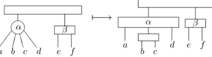
If, before being treated, α is a non-basic P-node with children β1, . . . βq, then Sα = Sβ1∪ . . . ∪ Sβq and
Sβ1, . . . Sβq are also intervals of S when S is sorted along a compatible order. The aim of the
SubTree-Insertion procedure is to make TK also respecting this condition. If D is Robinsonian and, if β is a
descendant of α, then, we are in one of the following two cases: 1. ∃ i ∈ [1, . . . , kα] such that Sβ⊂ Sαi.
2. ∃ i, j ∈ [1, . . . , kα], i < j such that:
• Sβ∩ Sαk = Sαk for i < k < j.
• Sβ∩ Sαk = ∅ for k < i or j < k.
In Case 2, we say that [νi, . . . , νj] is the intersection interval of β and, if β is a Q-node with children γ1, . . . , γp,
we can fix the orientation of the γi relatively to that of Sα1, Sα2, . . . , Sαkα. More precisely, up to a reversal of
the γi, we have:
∃ j1< j2< . . . jp+1 such that ∀i ∈ [1, . . . , p]:
If k < ji or k > ji+1, Sαk∩ Sγi = ∅.
If ji< k < ji+1, Sαk ⊂ Sγi.
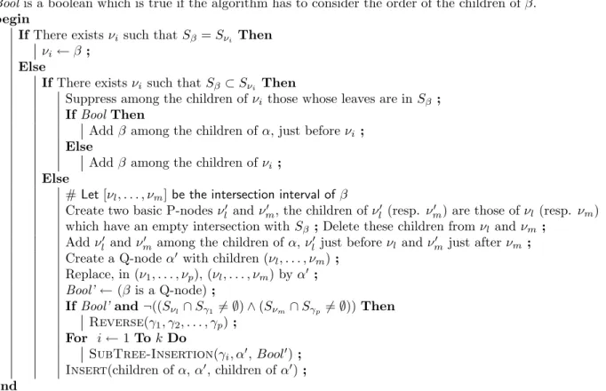
Procedure SubTree-Insertion(β, α, Bool) Input: α is a Q-node with children ν1, . . . , νp.
β is a node with children γ1, . . . , γk and such that Sβ⊂ Sα.
Bool is a boolean which is true if the algorithm has to consider the order of the children of β. begin
IfThere exists νi such that Sβ= Sνi Then
νi← β ;
Else
IfThere exists νi such that Sβ ⊂ Sνi Then
Suppress among the children of νi those whose leaves are in Sβ ;
IfBool Then
Add β among the children of α, just before νi ;
Else
Add β among the children of νi ;
Else
# Let [νl, . . . , νm] be the intersection interval of β
Create two basic P-nodes ν′
l and νm′ , the children of νl′ (resp. νm′ ) are those of νl (resp. νm)
which have an empty intersection with Sβ ;Delete these children from νl and νm ;
Add ν′
l and νm′ among the children of α, νl′ just before νl and νm′ just after νm;
Create a Q-node α′ with children (ν
l, . . . , νm) ;
Replace, in (ν1, . . . , νp), (νl, . . . , νm) by α′ ;
Bool’ ← (β is a Q-node) ;
IfBool’ and ¬((Sνl∩ Sγ1̸= ∅) ∧ (Sνm∩ Sγp̸= ∅)) Then
Reverse(γ1, γ2, . . . , γp) ;
For i ← 1 To k Do
SubTree-Insertion(γi, α′, Bool′) ;
Insert(children of α, α′, children of α′) ;
end
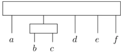
For example, with the dissimilarity D2of Figure 6, the algorithm, at Step 1, constructs the PQ-tree of Figure
7. D2 a b c d e f g h a b c d e f g h 0 2 2 2 2 2 4 6 0 1 1 2 2 3 6 0 1 2 2 3 6 0 2 2 3 5 0 1 3 5 0 3 4 0 1 0 " a b" c" d" e" f" g" h"
Figure 6: A dissimilarity and its sets Γ1(x)
At Step 2, from the P-node α of the PQ-tree in Figure 7 and the last two columns of the dissimilarity of Figure 6, the algorithm constructs the P-node α′ in Figure 7. Then, after SubTree-Insertion, the
a ✚✚ ✚✚✚ b ✧✧ c d ❜ ❜ ✐ e f ✒✑ ✓✏ α & & & & & & g h ♥ ❝ ❝ ❝ ❝❝ ✏ ✏ ✏ ✏ ✏ α′ a b c ✐ ! ❅ d e ✐ ! ❅ f
Figure 7: The PQ-tree built from the graph G1(D2) and the Q-node α′ built at Line 2 of Step 2
a b c ✐ ! ❅ d e f α g h ♥ ❝ ❝ ❝ ❝❝ ✏ ✏ ✏ ✏ ✏
Figure 8: The PQ-tree of the dissimilarity of Figure 6 after Step 2
We now give the complexity of this step: The procedure Refine does not change the order of the leaves. More precisely, within each Si
α, the order of the leaves is the same as the one in α (and thus as
the one in β). So, all the tests and operations in SubTree-Insertion take at most linear time. There are at most log(|Sβ|) recursive calls; thus, in step 2, the loop “forall child β of α such that |Sβ| > 1 do
SubTreeInsertion(β, α′, F alse)” takes O(log(|S
α|)). Thus the complexity of the treatment of one P-node
α is the complexity of Refine(Sα, Sα), which is O(p2), where p is the greatest of |Sα|, |Sα|. It is possible
for p to be in O(n), and there may exist O(n) P-nodes. But if we look at step 2 as a whole, each D(x, y) is used at most twice: one with x in a Sα and y in Sα, and one with y in a Sα′ and y in Sα′. So, step 2 runs
in O(n2) time. In addition, we have:
Property 7. Let α be a P-node of TK after Step 2. If D is Robinsonian with PQ-tree A, then there exists
a node α′ of A such that S
α′ = Sα.
Proof. Let α′ be the node of A such that S
α⊂ Sα′ and such that none of its children has this property. Let
us suppose that the claim is false, i.e. that Sα̸= Sα′. For any x ∈ S \ Sα, D(x, y) has a constant value for
y ∈ Sα. So, for every permutation represented by A, the reversal of Sα is possible. Thus α′ is a P-node
with children β1, . . . βk, . . . , βp, with k > 1 and Sα= Sβ1∪ . . . ∪ Sβk. There exists dα such that, for every
i ̸= j ∈ {1, . . . , p}, x ∈ Sβi, y ∈ Sβj, D(x, y) = dα. Let x ∈ Sα, we set I = {y ∈ S, D(x, y) ≤ dα}. The
Γ-interval I is contained in all the Γ-intervals containing Sα; in addition, Sα′ ⊂ I. The Γ-interval I has been
considered to construct TK (otherwise, α would be the root of TK). So (as Sα̸= I), there exist x ∈ S, d > 0
such that the Γ-interval J = {y ∈ S, D(x, y) ≤ d} contains points of Sα′ \ Sα and points of S \ Sα′ and is
such that J ∩ Sα= ∅. So, there exist y ∈ S \ Sα′, z ∈ Sα′ such that D(y, z) ≤ d. By Property 6, D(y, z′) ≤ d
for every z′∈ S
4.3
Treatment of Q-nodes (Step 3)
This step aims at checking, for every Q-node α whether α fulfills Property 6. For this step, we will consider all nodes with two children as Q-nodes. We first give some definitions and properties.
Let α be a Q-node and let β be a node which is not a descendant of α (i.e. either Sα ⊂ Sβ or
Sα∩ Sβ = ∅). We say that α is orientable with respect to β if there exist x, y in Sα and z in Sβ \ Sα
such that D(x, z) ̸= D(y, z).
Let α be a Q-node with children (γ1, . . . , γp). The two extreme points aα and bα of α are defined as
follows:
• if γ1 (resp. γp) is a leaf x, then x is aα (resp. bα).
• If γ1(resp. γp) is a P-node, we take for aα (resp. bα) any point of Sγ1 (resp. Sγp).
• If γ1(resp. γp) is a Q-node with extreme points x and y, we choose one of them for aα (resp. bα).
Claim 3. If a Q-node α is orientable with respect to a node β, then there exists z in Sβ \ Sα such that
D(aα, z) ̸= D(bα, z).
Proof. For any z in Sβ\ Sα, and any x, y in Sα, either D(aα, z) ≤ D(x, z) ≤ D(bα, z) and D(aα, z) ≤
D(y, z) ≤ D(bα, z) or D(aα, z) ≥ D(x, z) ≥ D(bα, z) and D(aα, z) ≥ D(y, z) ≥ D(bα, z). In both cases, if
D(x, z) ̸= D(y, z), then D(aα, z) ̸= D(bα, z).
For any pair of Q-nodes {α, β}, let us compare D(aα, aβ), D(aα, bβ), D(bα, aβ), D(bα, bβ). If Sαand Sβ
are disjoint, then, up to symmetry, we are in one of the following cases: • D(aα, aβ) = D(aα, bβ) = D(bα, aβ) = D(bα, bβ)
Then α and β are not orientable with respect to each other. • D(aα, aβ) < D(aα, bβ) and D(bα, aβ) < D(aα, aβ)
Then both α and β are orientable with respect to the other. In this case, if D is Robinsonian, for any ordering of S compatible with D, the quadruplet {aα, bα, aβ, bβ} is ordered as (aα, bα, aβ, bβ) or
(bβ, aβ, bα, aα).
• D(aα, aβ) = D(bα, aβ) < D(aα, bβ) = D(bα, bβ)
In this case, β is orientable with respect to α : if D is Robinsonian, for any ordering of S compatible with D, the quadruplet {aα, bα, aβ, bβ} is ordered as (aα, bα, aβ, bβ), (bα, aα, aβ, bβ), (bβ, aβ, bα, aα) or
(bβ, aβ, aα, bα).
It could be possible, even when D is Robinsonian, that, for a point x of Sβ\ {aβ, bβ}, we have
D(x, bα) < D(x, aα) (for example, with Sα= {aα, bα}, Sβ = {aβ, x, bβ}, D(aα, aβ) = D(bα, aβ) = 1,
D(aα, bβ) = D(bα, bβ) = 4, D(x, bα) = 2 and D(x, aα) = 3). If this is the case, α is also orientable
relatively to β, that is to say that, if D is Robinsonian, for any ordering of S compatible with D, {aα, bα, aβ, bβ} is ordered as (aα, bα, aβ, bβ) or (bβ, aβ, bα, aα). We then say that α is orientable via an
internal point of β. If α is orientable via an internal point of β, we define the dissimilarity D′ on S by:
– if x ̸= aα and y ̸= aβ, then D′(x, y) = D(x, y)
– D′(a
α, aβ) = D′(aα, aβ) + ϵ, where ϵ is a positive real, small enough not to interfere with the other
values of D. For instance, if all the values of D are integer, we can take ϵ = 0.1.
Claim 4. D′ is Robinsonian if and only if D is Robinsonian; in addition, if D and D′ are Robinsonian,
they have the same set of compatible permutations.
The advantage of D′ upon D is that, at Step 4, the algorithm needs to consider only the extreme points of
the sets Sα.
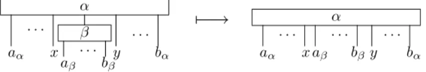
• If β is not an extreme child of α and if D(aα, aβ) < D(aα, bβ) or D(bα, aβ) > D(vα, bβ), then β is
orientable with respect to α. In this case, it is possible to delete β from T , that is to say to replace, among the children of α, β by its children (see Figure 9).
α aα . . . x β aβ . . . bβ y . . . bα aα . . . x aβ . . . bβy . . . bα α
.−→
Figure 9: Deletion of a child of a Q-node This transformation corresponds to Insert(children of α, β, children of β). • D(aα, aβ) = D(aα, bβ) and D(bα, aβ) = D(bα, bβ).
It may be possible that, for a point x in Sα\ (Sβ∪ {aα, bα}), D(x, aβ) ̸= D(x, bβ); in fact, we are then
in the previous case and it is possible to delete β from T . As before, we shall say that β is orientable via an internal point.
• If β is an extreme child of α, for instance the last one, and if D(aα, aβ) < D(aα, bβ), then, as in the
first case, β is orientable with respect to α and it is possible to delete β from T via the transformation of Figure 10. After this transformation, bαhas to be equal to bβ, although, before the transformation,
α aα . . . . x β aβ . . . bβ aα . . . . x aβ . . . bβ α
.−→
Figure 10: Deletion of a extreme child of a Q-node bαcan be equal to aβ or bβ.
• β is an extreme child of α, for instance the last one, and D(aα, aβ) = D(aα, bβ).
It may be possible that, for a point x in Sα\ (Sβ∪ {aα}), D(x, aβ) ̸= D(x, bβ); we shall say that β is
orientable with respect to α via an internal point. In fact, we are then in the previous case and it is possible to delete β from T .
We have the following properties:
Claim 5. Let α be a Q-node orientable with respect to a P-node β. Then, for any x ∈ Sβ, D(x, aα) ̸=
D(x, bα).
Proof. After Step 2, both D(x, aα) and D(x, bα) has a constant value for all x ∈ Sβ.
Claim 6. Let α be a Q-node, child of a P-node β and γ be a node such that Sγ ∩ Sβ = ∅, then α is not
orientable with respect to γ. In addition, if α is orientable, it is orientable with respect to β or to a descendant of β.
Proof. Since aαand bαare in Sβ, after Step 2, for every x in S \ Sβ, D(x, aα) = D(x, bα).
Claim 7. Let α be a Q-node orientable with respect to a node β and γ be an ancestor of β. Then α is orientable with respect to to γ.
Proof. As α is orientable with respect to β, there exists x ∈ Sβ such that D(aα, x) ̸= D((bα, x). Since
Property 8. Let α and β be Q-nodes, α being a child of β. If α is orientable (with respect to β or to another node), then it can be deleted.
Proof. If α is orientable with respect to a child of β, then, by Claim 7, α is orientable with respect to β and thus can be deleted from T . If α is orientable with respect to a node γ and not with respect to β, there exists z in Sγ\Sβsuch that D(aα, z) ̸= D(bα, z) (let us suppose, for instance, that D(aα, z) < D(bα, z)). As aαand
bαare in Sβ, β is orientable with respect to γ. So, we have either D(aβ, z) ≤ D(aα, z) < D(bα, z) ≤ D(bβ, z)
or D(bβ, z) ≤ D(aα, z) < D(bα, z) ≤ D(aβ, z). In both cases, α can be deleted from T .
We recall that a node α is said to be K-big if |Sα| > K. A node β, child of a P-node α, is said to be
K-closed if ΓK(x) ̸⊂ Sβ for all x ∈ Sβ; otherwise, β is said to be K-free.
Property 9. Let α be an orientable Q-node. If α cannot be deleted from T , then: • α is a K-big child of a P-node γ.
• γ has a K-big child β such that α is orientable with respect to β.
Proof. By Property 8, α is the child of a P-node γ. By Claims 6 and 7 α is orientable with respect to γ. Let x in Sγ be such that D(x, aα) ̸= D(x, bα), there exists a child β of γ such that x ∈ Sβ; α is orientable with
respect to β.
Let us suppose that β is a K-closed node, then, by Property 5, for every y in Sβ, D(y, z) has a constant
value on Sγ\ Sβ. It would be impossible that D(x, aα) ̸= D(x, bα). So β is a K-free child of γ; by Property
4, β is K-big.
Let us suppose that α is a K-closed node, D(aα, x) and D(bα, x) are K-known, and they are different. So,
among the permutations which are compatible with the K-known values of D, we can have (aα< bα< x)
or (bα < aα < x) but not both. But after step 1, T represents the set of permutations of S which are
compatible with the K-known values of D. For these orders, we can reverse the aαand bαwithout changing
the place of x. So both (aα< bα< x) and (bα < aα< x) appear in the permutations compatible with T .
So α is a K-free child of γ; by property 4, α is K-big. We can now give the pseudo-code of step 3: step 3: Treatment of Q-Nodes
Output: A subset S′ of S.
begin
Compute-Extreme-Points ;
ForAllQ-node α (# T is traversed in postorder) Do Q-Node-Examination(α) ;
end
Compute-Extreme-Points computes aα and bα for each Q-node α and Q-Node-Examination deletes
Q-nodes that can be deleted or changes D when a Q-node is orientable via an internal point.
We now give an example to illustrate this step. If we consider the dissimilarity D1 of Figure 4 and its
PQ-tree after Step 2 (see Figure 5), at Step 3, since D1(b, f ) < D1(a, f ) (a and b are the extreme points of
α) and D1(a, e) < D1(a, f ), both α and β are deleted and this PQ-tree is transformed into the PQ-tree of
Figure 11.
a
b c d e f
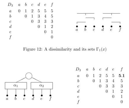
We now consider the dissimilarity D3 (see Figure 12). At Step 1, the algorithm builds the PQ-tree of
Figure 13, which remains unchanged at Step 2. At Step 3, since α2 is orientable via an internal point of α1
(namely b), the dissimilarity D3 is changed into the one of Figure 13.
D3 a b c d e f a b c d e f 0 1 2 5 5 5 0 1 3 4 5 0 3 3 3 0 1 2 0 1 0 " a b" c" d" e" f"
Figure 12: A dissimilarity and its sets Γ1(x)
" a b" c" d" e" f" α1 ✟✟✟ α2 ❍ ❍ ❍ ♥ Da3 b c d e f a b c d e f 0 1 2 5 5 5.1 0 1 3 4 5 0 3 3 3 0 1 2 0 1 0
Figure 13: The PQ-tree built from the graph G1(D3) and the dissimilarity D3after Step 3
In worst case, Q-Node-Examination(α) compares D(x, aα) and D(x, bα) for all x in S \ Sα. So
Q-Node-Examinationruns in O(n) time. As T cannot have more than n Q-nodes, this step runs in O(n2)
time.
4.4
Recursive Calls and Merging (Step 4)
This step aims at orienting Q-nodes if applicable. An orientable Q-node is the child of a P-node, and, by Property 7, these P-nodes can be treated independently. We denote by D|S′ the dissimilarity D applied on
a subset S′ of S. The pseudo-code of this step is the following:
step 4: Recursive Calls and Merging begin
ForAllK-big P-node α (# T is traversed in postorder) Do S′
α ← Representatives(α) ;
If |S′
α| > 2 Then
# Otherwise, there is no Q-node to orient Apply the whole algorithm (steps 1—5) to D|S′
α ;
IfD|S′
α is not Robinsonian Then
Stop ;# D is not Robinsonian Else # T′ is the PQ-tree of D| S′ α Merging(α, T′) ; end
• aβ and bβ for each K-big Q-node β which is a child of α.
• An element of Sγ for each K-big P-node γ which is a child of α.
By Properties 4 and 5, there is no need to consider K-small children of α (if D is Robinsonian and β is a K-small child of α, then β is a node of the PQ-tree A of D; in addition, if α′ is the node of A such that
Sα′ = Sα, then β is (in A) a child of α′). Since D has been changed at Step 3, by Claim 4, it is sufficient
to consider D|S′α. The aim of Merging is to rearrange T (α) according to what has been done during the
recursive call on α. Its pseudo-code is : Procedure Merging(α, T′)
Inputα is a P-node.
T′ is a PQ-tree on a subset of S α.
begin
If Not all the subtrees of T′ are leaves or Q-nodes with two leaves a
β and bβ, where β is a Q-node of T
Then
# Otherwise, no Q-node has been oriented ForAllK-big child γ of α Do
Ifγ is a P-node Then
# Let x be the representative of γ, x is a leaf of T′
Replace, in T′, x by γ ;
Ifγ is a Q-node Then
# Let aγ and bγ be the representatives of γ
# aγ and bγ are leaves of T′ and are consecutive children of a Q-node ξ
# Let ν1, . . . , νp be the children of γ
Replace, among the children of ξ, aγ, bγ by ν1, . . . , νp;
Ifα has K-small children η1, . . . , ηq Then
IfThe root of T′ is a P-node or a Q-node with two children Then
Add η1, . . . , ηq among the children of the root of T′ ;
# If the root of T′ is a Q-node with two children, it becomes a P-node
Replace α by T′ ;
Else
Delete the K-big children of α ; Add T′ among the children of α ;
Else
Replace α by T′ ;
end
We now give the complexity of this step. Merging(α, T′) runs in O(|S
α|) time, so, at this step, the calls of Merging not in recursive calls are,
altogether, in O(n2).
Let us calculate the total number of representatives.
There are less than n/K K-big nodes with no K-big descendants, and thus less than n/K K-big nodes with more than two K-big descendants such that none of the two is a descendant of the other.
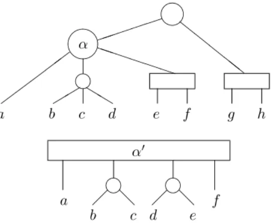
Let α be a node with only one K-big descendant β. If both α and β have representatives, then the parent of β is a P-node with more than two children and α is a Q-node. So Sα\ Sβ contains at least three elements
(see Figure 14).
Since a Q-node has at most two representatives, and a P-node at most one : "
α
|S′
α| ≤ 2 × n/3 + 4 × n/K
We shall see below that step 5 (as steps 1— 3) runs in O(n2) time. By taking K > 12, we get#
α|Sα′| <
♥ β ♥ ✡✡ ✡ ( ❏❏ ❏ ( α ( Figure 14:
4.5
Verification (Step 5)
If D is Robinsonian, after Step 4, T represents the set of all the permutations compatible with D and any permutation represented by T corresponds to a linear ordering. Conversely, if D is not Robinsonian, Steps 1—4 of the algorithm may produce a PQ-tree: for instance, in Step 3, we do not check if there is some contradiction between the orientations of the Q-nodes. In this case, no permutation on S corresponds to a linear ordering. So, the algorithm has to check if D is actually Robinsonian.
To do that, the algorithm has only to choose a permutation among the ones compatible with T and verify that it corresponds to a linear ordering, that is to say to verify that every row and every column is not decreasing when starting from the diagonal. This step runs in O(n2) time.
5
A complete example
We now show on an example how our algorithm runs. Let us consider the following dissimilarity:
D x1 x2 x3 x4 x5 x6 x7 x8 x9 x10x11x12x13x14x15x16x17x18x19 x1 0 9 2 11 6 11 6 6 9 11 6 11 6 5 11 11 9 11 6 x2 0 9 11 2 11 3 6 1 11 6 11 6 9 11 11 1 11 3 x3 0 11 6 11 6 6 9 11 6 11 6 1 11 11 9 11 6 x4 0 11 8 11 11 11 8 11 8 11 11 1 8 11 2 11 x5 0 11 3 4 2 11 4 11 4 6 11 11 2 11 1 x6 0 11 11 11 1 11 5 11 11 6 3 11 6 11 x7 0 4 3 11 4 11 4 6 11 11 3 11 2 x8 0 5 11 1 11 3 4 11 11 5 11 4 x9 0 11 5 11 6 9 11 11 1 11 3 x10 0 11 5 11 11 7 2 11 6 11 x11 0 11 2 4 11 11 5 11 4 x12 0 11 11 2 5 11 1 11 x13 0 4 11 11 6 11 4 x14 0 11 11 9 11 6 x15 0 7 11 1 11 x16 0 11 7 11 x17 0 11 3 x18 0 11 x19 0
We take, for this example, K = 2. The intervals Γ1(xi) and Γ2(xi) are represented in Figure 15:
In Figure 15, the intervals Γ1(xi) and Γ2(xi) are represented with a vertical line above xi. When Γ1(xi) = Γ1(xj)
(or Γ2(xi) = Γ2(xj)), the interval is represented once, but if Γ1(xi) = Γ2(xj), the interval is represented twice. To
construct these intervals (or, more precisely, the vertex-clique incidence matrix of G2(D)), we have used the values
in italic of the matrix D.
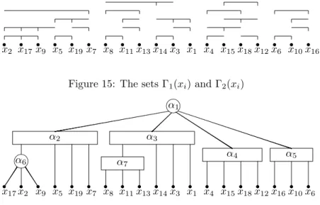
• At Step 1 (from the vertex-clique incidence matrix of G2(D)), we construct the PQ-tree T (see Figure 16).
)
x2 x)17x)9 x)5 x)19x)7 x)8 x)11x)13x)14x)3 x)1 x)4 x)15x)18x)12x)6 x)10x)16
Figure 15: The sets Γ1(xi) and Γ2(xi)
) x17x)2 x)9 x)5 x)19x)7 x)8 x)11x)13x)14x)3 x)1 x)4 x)15x)18x)12x)16x)10x)6 ❧ α6 α2 α7 α3 α4 α5 ❧ α1
Figure 16: The PQ-tree T after Step 1
– On α6, because of D(x2, x11) > D(x17, x11) = D(x9, x11) ≥ D(x5, x11), we do the transformation of
Figure 17. " x17 " x2 " x9 ✍✌ ✎☞ α6
.−→
" x2 " x17 ✁✁ " x9 ❆ ❆ ✍✌ ✎☞ α8 α′ 6 Figure 17:– Since for all i ̸= 17, 9, D(xi, x17) = D(xi, x9), α8 remains a P-node.
• At Step 3:
– Since D(x2, x8) > D(x9, x8), α′6 is orientable with respect to α3 and, by property 8, it can be deleted
from T . As D(x2, x8) > D(x5, x8), α2 is transformed into the Q-node of Figure 18.
" x2 " x17 ✁✁ " x9 ❆ ❆ " x5 " x19 " x7 ✍✌ ✎☞ α8 α2 Figure 18:
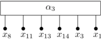
– Since D(x9, x8) < D(x9, x13), α7 is orientable. As its parent is a Q-node, it can be deleted from T . As
D(x9, x8) < D(x9, x1), α3is transformed into the Q-node of Figure 19.
– Since D(x4, x6) = D(x4, x16) > D(x12, x6) = D(x12, x16), α4 is orientable and, in order to check if α5 is
orientable, we have to consider the interior points of Sα4. Since D(x15, x6) < D(x15, x16), α5is orientable
" x8 " x11 " x13 " x14 " x3 " x1 α3 Figure 19: – Since D(x2, x4) = D(x2, x12) = D(x7, x4) = D(x7, x12) D(x2, x6) = D(x2, x16) = D(x7, x6) = D(x7, x16) D(x8, x4) = D(x8, x12) = D(x1, x4) = D(x1, x12) D(x8, x6) = D(x8, x16) = D(x1, x6) = D(x1, x16) (D(x2, x8) < D(x2, x1)) ∧ (D(x2, x1) > D(x7, x1))
nothing else has to be done at this step. • At Step 4:
α2, α3, α4 and α5 are K-big, and they are all children of the P-node α1.
S′
α1= {x1, x2, x4, x6, x7, x8, x12, x16}.
D|S′
α1 and the sets Γ1(xi) and Γ2(xi) are represented in Figure 20.
D|S′ α1 x1 x2 x4 x6 x7 x8 x12 x16 x1 0 9 11 11 6 6 11 11 x2 0 11 11 3 6 11 11 x4 0 8 11 11 8 8 .1 x6 0 11 11 5 3 x7 0 4 11 11 x8 0 11 11 x12 0 5 x16 0 " x2 " x7 " x8 " x1 " x4 " x12 " x6 " x16
Figure 20: The dissimilarity D|S′
α1 and its sets Γ1(x) and Γ2(x)
– We first construct the PQ-tree T′of G 2(D|S′
α1) (see Figure 21).
– On D|S′
α1, nothing has to be done at Steps 2 and 3.
– At Step 4, the algorithm works on D|S′
β1, where S
′
β1 = {x2, x1, x4, x16}. The sets Γ1(xi) and Γ2(xi)
(for D|S′
β1) and the PQ-tree T ” of G2(D|S′β1) are represented in Figure 22. The PQ-tree T ” is not
transformed by the algorithm, and so T′′ is (definitively) the PQ-tree of D| S′
β1. The merging of T
′ with
T′′ does not change T′ which is thus the PQ-tree of D| S′
α1. The merging of T with T
′ induces the
following transformations on T :
" x2 " x7 " x8 " x1 " x4 " x12 " x6 " x16 β2 β3 ♥ β1 ✟✟✟ ❍❍❍
Figure 21: The PQ-tree T′ for D| S′ α1 after Step 1 " x2 " x1 " x4 " x16 " x2 " x1 " x4 " x16 γ2 γ3 ♥ γ1 ✟✟✟ ❍❍❍
Figure 22: The sets Γ1(x) and Γ2(x) for D|S′
β1 and the PQ-tree of D|S′β1
" x2 " x17 " x9 " x5 " x19 " x7 " x8 " x11 " x13 " x14 " x3 " x1 ♥ α8 ✄✄ ❈❈ β′ 2 Figure 23: " x4 " x15 " x18 " x12 " x6 " x10 " x16 β′ 3 Figure 24:
So, we obtain the PQ-tree of Figure 25 as a potential PQ-tree for D.
) x2 x)17x)9 x)5 x)19x)7 x)8 x)11x)13x)14x)3 x)1 ❧ α8 ✄✄ ❈❈ β′ 2 ) x4 x)15x)18x)12x)6 x)10x)16 β′ 3 ❧ α1 ! ! ❅❅ ❅
Figure 25: The PQ-tree T after Step 4
• At step 5, the algorithm checks that one of the permutations represented by the PQ-tree of Figure 25 cor-responds to a linear order. This is the case because, when {x1, x2, . . . , x19} is sorted along the permutation
columns not decreasing from the diagonal: D x2 x17x9 x5 x19x7 x8 x11x13x14x3 x1 x4 x15x18x12x6 x10x16 x2 0 1 1 2 3 3 6 6 6 9 9 9 11 11 11 11 11 11 11 x17 0 1 2 3 3 5 5 6 9 9 9 11 11 11 11 11 11 11 x9 0 2 3 3 5 5 6 9 9 9 11 11 11 11 11 11 11 x5 0 1 2 4 4 4 6 6 6 11 11 11 11 11 11 11 x19 0 2 4 4 4 6 6 6 11 11 11 11 11 11 11 x7 0 4 4 4 6 6 6 11 11 11 11 11 11 11 x8 0 1 3 4 6 6 11 11 11 11 11 11 11 x11 0 2 4 6 6 11 11 11 11 11 11 11 x13 0 4 6 6 11 11 11 11 11 11 11 x14 0 1 5 11 11 11 11 11 11 11 x3 0 2 11 11 11 11 11 11 11 x1 0 11 11 11 11 11 11 11 x4 0 1 2 8 8 8 8 x15 0 1 2 6 7 7 x18 0 1 6 6 7 x12 0 5 5 5 x6 0 1 3 x10 0 2 x16 0
6
Some other applications
Let M be an n×k nonnegative matrix containing m nonzeros. The doubly lexical ordering problem consists to permute the rows and the columns of M in such a way that both the row vectors and the column vectors are in nondecreasing lexicographic order (see Lubiw 1985). There exists an O(m · log(n + k) + k) algorithm for this problem (see Paige and Tarjan 1987). When M is a 0-1 matrix, the same problem can be solved in O(n · k) time (see Spinrad 1993).
We consider here a strict version of doubly lexical ordering: we say that M admits a 2D-ordering if it is possible to permute the rows and the columns of M in such a way that all the rows and columns are in nondecreasing order. We remark that, contrary to the doubly lexical ordering, some matrices do not admit a 2D-ordering (for instance »
0 1
1 0
–
). Given an n × k positive matrix M , the following (n + k) × (n + k) dissimilarity DM is Robinsonian if and
only if M admits a 2D-ordering:
0 .. . . .. . . . . .. . . . . .. 0
M
0
0
In addition, if DM is Robinsonian, since M is positive, for any compatible permutation, the first n entries are not
mixed with the last k ones. So, the permutations (on the n+k entries) compatible with this Robinsonian dissimilarity are exactly the ones for which M is 2D-ordered.
So, our algorithm can be adapted to this problem: Given an (n × k) non negative matrix M :
1. Check if the dissimilarity D(M ) = »
0 M+ E
Mt+ E 0
–
is Robinsonian (E is the matrix defined by setting E[i, j] = 1 for all i, j).
2. If D(M ) is Robinsonian, then any compatible ordering of D(M ) corresponds to a 2D-ordering of M . Otherwise, a 2D-ordering of M does not exist.
This algorithm solves the 2D-ordering problem in O((n + k)2
), which is optimal in worst case (i.e. when M is dense and n ≈ k).
An ultrametric is a distance D on a set S such that for any x, y and z in S, D(x, y) ≤ max{D(x, z), D(y, z)}. Ultrametrics have many applications in classification because they are in one-to-one correspondence with hierarchies (see Barth´elemy and Gu´enoche 1991 and Critchley and Fichet 1994). Ultrametrics are a particular case of Robinsonian dissimilarities. More precisely, they are the Robinsonian dissimilarities for which the PQ-tree has only P-nodes (see Seston 2008b). Our algorithm can be adapted to ultrametrics recognition:
Given a dissimilarity D:
1. Check if D is Robinsonian.
2. If D is Robinsonian, verify that its PQ-tree has only P-nodes.
This algorithm runs in O(n2), where n is the number of elements of S, which is optimal.
Let D be a dissimilarity on an n-set S, and k an integer in [0, . . . , n − 1]. We define the dissimilarity Dk by:
Dk(x, y) = D(x, y) if D(x, y) is k-known (i.e. if x ∈ Γ
k(y) or y ∈ Γk(x)).
Dk(x, y) = ∞ otherwise.
We say that D is k-Robinsonian if Dk is Robinsonian. Equivalently, D is k-Robinsonian if its graph G k is
an interval graph. This generalizes Robinsonian dissimilarities, since (n − 1)-Robinsonian is equivalent to Robinsonian. In addition, every dissimilarity is 0-Robinsonian and if a dissimilarity D is k-Robinsonian, then D is (k − 1)-Robinsonian. So, with a dichotomic search, it is possible to determine, in O(n2log n), the
greatest k such that D is k-Robinsonian.
References
J.P. Barth´elemyand F. Brucker (2003), “NP-Hard Approximation Problems in Overlapping Cluster-ing”, Journal of Classification 18, 159–183.
J.P. Barth´elemyand A. Gu´enoche (1991), Trees and Proximity Representations, J. Wiley & sons. S. Benzer(1962), “The Fine Structure of the Gene”, Scientific American 206:1, 70–84.
M.W. Berry, B. Hendrickson and P. Raghavan (1996), “Sparse Matrix Reordering Schemes for Browsing Hypertext”, in The Mathematics of Numerical Analysis, J. Renegar, M. Shub and S. Smale Eds., pp 99–123, American Mathematical Society, Lectures in Applied Mathematics.
L. Boneva(1980), “Seriation with Applications in Philology”, in Mathematical Statistics, R. Bartoszy´nski, J. Koronacki and R. Zieli´nski Eds., pp 73–82, PWN Polish Scientific Publishers.
K.S. Booth(1975), PQ-Tree Algorithms, Ph.D. Thesis, University of California.
K.S. Boothand G.S. Lueker (1976), “Testing for the Consecutive Ones Property, Interval Graphs and Graph Planarity Using PQ-Tree Algorithm”, Journal of Computer and System Sciences 13, 335–379. M.J. Brusco(2002), “A Branch-and-Bound Algorithm for Fitting Anti-Robinson Structures to Symmetric
Dissimilarity Matrices”, Psychometrica 67, 459–471.
G. Caraux and S. Pinloche (2005), “PermutMatrix: a Graphical Environment to Arrange Gene Ex-pression Profiles in Optimal Linear Order”, Bioinformatics 21, 1280–1281.
C.H. Chen, H.G. Hwu, W.J. Jang, C.H. Kao, Y.J. Tien, S. Tzengand H.M. Wu (2004), “Matrix Visualisation and Information Mining”, COMPSTAT’2004, Prague.
V. Chepoiand B. Fichet (1997), “Recognition of Robinsonian Dissimilarities”, Journal of Classification 14, 311–325.
V. Chepoi, B. Fichet and M. Seston (2009), “Seriation in the Presence of Errors: NP-Hardness of l∞-Fitting Robinson Structures to Dissimilarity Matrices”, Journal of Classification 26, 279–296.
V. Chepoi and M. Seston (2011), “Seriation in the Presence of Errors: A Factor 16 Approximation Algorithm for l∞-Fitting Robinson Structures to Distances”, Algorithmica 59, 521–568.
F. Critchley and B. Fichet (1994), “The Partial Order by Inclusion of the Principal Classes of Dis-similarities on a Finite Set, and Some of Their Basic Properties”, in Classification and Dissimilarity Analysis, B. Van Cutsem Ed., pp 5–65, Springer Verlag, Lecture Notes in Statistics.
E. Diday(1986), “Orders and Overlapping Clusters by Pyramids”, in Multidimensionnal Data Analysis, J. de Leeuw, W. Heiser, J. Meulman and F. Critchley Eds., pp 201–234. DSWO.
C. Durandand B. Fichet (1988), “One-to-One Correspondences in Pyramidal Representation: an Unified Approach”, in Classification and Related Methods of Data Analysis, H.H. Bock Ed., pp 85–90. North-Holland.
D.R. Fulkersonand O.A. Gross (1965), “Incidence Matrices and Interval Graphs”, Pacific Journal of Mathematics 15, 835–855.
P.C. Gilmoreand A.J. Hoffman (1964), “A Characterization of Comparability Graphs and of Interval Graphs”, Canadian Journal of Mathematics 16, 539–548.
M.C. Golumbic(1980), Algorithmic Graph Theory and Perfect Graphs, Academic Press.
M. Habib, R. McConnell, C. Paul and L. Viennot (2000), “Lex-BFS and partition refinement, with applications to transitive orientation, interval graph recognition and consecutive ones testing”, Theoretical Computer Science 234, 59–84.
D. Halperin(1994), “Musical Chronology by Seriation”, Computer and the Humanities 28, 13–18. V. Heun(2008), “Analysis of a Modification of Gusfield’s Recursive Algorithm for Reconstructing
Ultra-metric Trees”, Information Processing Letters 108, 222–225.
L. Hubert(1974), “Some Applications of Graph Theory and Related Nonmetric Techniques to Problems of Approximate Seriation: The Case of Symmetric Proximity Measures”, British Journal of Mathematical and Statistical Psychology 27, 133–153.
D.G. Kendall(1969), “Incidence Matrices, Interval Graphs and Seriation in Archeology”, Pacific Journal of Mathematics 28:3, 565–570.
A. Lubiw(1985), “Doubly Lexical Orderings of Matrices”, Proceedings of the 17th Annual ACM Symposium on the Theory of Computing, 396–404.
G.S. Lueker(1975), Interval Graph Algorithms, Ph.D. Thesis, Princeton University.
I. Mikl´os, I. Somodi and J. Podani (2005), “Rearrangement of Ecological Data Matrices via Markov Chain Monte Carlo Simulation”, Ecology 86:12, 39–49.
B. Mirkinand S. Rodin (1984), Graphs and Genes, Springer-Verlag.
R. Paigeand R.E. Tarjan (1987), “Three Partition Refinement Algorithms”, SIAM Journal on Com-puting 16, 973–989.
W.M.F. Petrie(1899), “Sequences in Prehistoric Remains”, Journal of the Anthropological Institute of Great Britain and Ireland 29, 295–301.
An-M. Seston(2008a), “A Simple Algorithm to Recognize Robinsonian Dissimilarities”, COMPSTAT’2008, Porto.
M. Seston (2008b), Dissimilarit´es de Robinson : Algorithmes de Reconnaissance et d’Approximation, Ph.D. Thesis, Universit´e de la M´editerran´ee.
J.P. Spinrad (1993), “Doubly Lexical Ordering of Dense 0-1 Matrices”, Information Processing Letters 45, 229–235.
A. Strehland J. Ghosh (2003), “Relationship-Based Clustering and Visualization for High-Dimensional DataMining”, INFORMS Journal on Computing 15, 208–230.