Stand-alone water current generator for OEB

(1)

Publisher’s version / Version de l'éditeur:

L’accès à ce site Web et l’utilisation de son contenu sont assujettis aux conditions présentées dans le site

Student Report; no. SR-2009-28, 2009-12-18

READ THESE TERMS AND CONDITIONS CAREFULLY BEFORE USING THIS WEBSITE.

https://nrc-publications.canada.ca/eng/copyright

NRC Publications Archive Record / Notice des Archives des publications du CNRC :

https://nrc-publications.canada.ca/eng/view/object/?id=9658557b-d08f-4bd6-918f-a8cb93339fb4 https://publications-cnrc.canada.ca/fra/voir/objet/?id=9658557b-d08f-4bd6-918f-a8cb93339fb4

NRC Publications Archive

Archives des publications du CNRC

For the publisher’s version, please access the DOI link below./ Pour consulter la version de l’éditeur, utilisez le lien DOI ci-dessous.

https://doi.org/10.4224/18253443

Access and use of this website and the material on it are subject to the Terms and Conditions set forth at Stand-alone water current generator for OEB

(2)

National Research Council Canada Institute for Ocean Technology Conseil national de recherches Canada Institut des technologies oc ´eaniques

SR-2009-28

Student Report

Stand -Alone Water Current Generator for OEB.

Li, L. F.

Li, L. F., 2009. Stand -Alone Water Current Generator for OEB. St. John's, NL : NRC Institute for Ocean Technology. Technical Report, SR-2009-28

(3)

DOCUMENTATION PAGE REPORT NUMBER

SR-2009-28

NRC REPORT NUMBER DATE

December 18, 2009

REPORT SECURITY CLASSIFICATION

Unclassified

DISTRIBUTION

Unlimited

TITLE

STAND-ALONE WATER CURRENT GENERATOR FOR OEB AUTHOR(S)

Lian Feng Li

CORPORATE AUTHOR(S)/PERFORMING AGENCY(S)

National Research Council, Institute for Ocean Technology, St. John’s, NL

PUBLICATION

SPONSORING AGENCY(S)

IOT PROJECT NUMBER NRC FILE NUMBER

KEY WORDS CFD, Current, Wave PAGES 38 FIGS. 13 TABLES SUMMARY

Ocean is usually consisted of complicated waves and currents motions. Thus waves and currents are always very important topics in fluid hydrodynamics. Waves and currents and their consequent interactions play a very important role in most of the ocean dynamic processes. So it is crucial to understand the effects of waves on currents and vice versa in the laboratory to design any ocean structure. Equipment that can generate vertically distributed uniform current would be an important tool for relevant model testing in the Offshore Engineering Basin (OEB) of IOT. The aim of this project is to study different physical characteristics of a current generator, such as its height, nozzle length, diameters of different sections, inlet size, single and multiple impeller-type and impeller characteristics that would provide best possible performance of the current flow. This final equipment would be a portable one and can be placed at any location and directions in the OEB. Flow-3D CFD code is used to simulate those characteristics. Results are shown in a systematic ways. An example is also given that shows how a current can reduce the height of an incoming wave field.

ADDRESS National Research Council

(4)

National Research Council Conseil national de recherches

Canada Canada

Institute for Ocean Institut des technologies

Technology océaniques

STAND-ALONE WATER CURRENT GENERATOR FOR OEB

SR-2009-28

Lian Feng Li

(5)

SUMMARY

Ocean is usually consisted of complicated waves and currents motions. Thus waves and currents are always very important topics in fluid hydrodynamics. Waves and currents and their consequent interactions play a very important role in most of the ocean dynamic processes. So it is crucial to understand the effects of waves on currents and vice versa in the laboratory to design any ocean structure . Equipment that can generate vertically distributed uniform current would be an important tool for relevant model testing in the Offshore Engineering Basin (OEB) of IOT. The aim of this project is to study different physical characteristics of a current generator, such as its height, nozzle length, diameters of different sections, inlet size, single and multiple impeller-type and impeller characteristics that would provide best possible performance of the current flow. This final equipment would be a portable one and can be placed at any location and directions in the OEB. Flow-3D CFD code is used to simulate those characteristics. Results are shown in a systematic ways. An example is also given that shows how a current can reduce the height of an incoming wave field.

(6)

TABLE OF CONTENTS

1 INTRODUCTION--- 1

2 CFD-FLOW 3D--- 1

2.1 Impeller --- 1

2.2 Input Variables--- 2

2.3 Mesh and Boundary --- 2

3 COMPUTATIONAL PROCEDURES --- 4

4 ANALYSES OF SINGLE IMPELLER MODELS --- 5

4.1 Nozzle Analysis --- 5

4.2 Model Shape Selection --- 6

4.3 Model Height Research--- 7

4.4 Analysis of Impeller Spin Rate --- 8

4.5 Single Impeller Model with Multiple Outlets--- 9

5 ANALYSES OF MULTIPLE IMPELLERS MODELS---10

5.1 An Application of Wave-current Interaction ---11

6 CONCLUSIONS ---12

REFERENCES---13

APPENDICES ---14

LIST OF FIGURES Figure 1: Leaking water in a pipe--- 3

Figure 2: Computational locations on an S shape model --- 4

Figure 3: Result image and current velocity plot for nozzle outlet diameter changing --- 5

Figure 4: Result image and current velocity plot for nozzle length changing--- 6

Figure 5: U shape, LL shape and S shape models --- 6

Figure 6: Result image and current velocity plot for different shapes --- 7

Figure 7: Result image and current velocity plot for different models’ height --- 8

Figure 8: Result image and current velocity plot for different impeller spin rate --- 9

Figure 9: Result images of single impeller model with two outlets ---10

Figure 10: Result images of 10 impellers’ model---10

Figure 11: Result images of 6 impellers’ model ---11

Figure 12: Result images of wave-current interaction (6 outlets) ---11

(7)

1 INTRODUCTION

This project is to develop a portable water current generator to be used for different model tests in the Offshore Engineering Basin (OEB), such as, wave-current interaction, suppress of the wave heights of an incoming wave fields, etc. A mechanical device activated by electric power is designed to generate water currents that have different directions with incoming waves. The generated currents interact with the waves and modify the flow kinematics. In some special case a current can be treated as a temporary breakwater.

A current-related model is created to study the current generation and propagation in the Offshore Engineering Basin (OEB). OEB is used to test the offshore and coastal structures, and the performance of ocean vehicle and equipment under a variety flow condition, such as, waves and currents to validate relevant theories and numerical models. For the present study, a relevant numerical model is created with impellers and a series of nozzles parallel to each other, and is developed to generate currents in the Flow 3D environment. The model is submerged, and its impeller can generate uniform water currents. This study is carried out through simulating different nozzles, shapes and other parameters of the current generator. Based on the Eulerian method that centralizes a spatial location and analyzes passing particles as the time changes. Results are shown in term of physical characteristic of the current generator itself and the outputs

2 CFD-FLOW 3D

Computational Fluid Dynamics (CFD) is an application of numerical methods to fluid mechanics. According to physical experiments and theories, CFD simplifies the physical model into a numerical model to develop and complete an analytic method. The research approach of CFD is to use a computer’s calculation and image to create a numerical simulation. The numerical simulation outputs detailed information of a fluid experiment without using any lab instruments. The resulting data is processed and converted into an output test result image, which is distributed with different colors. Flow 3D is a CFD software which is installed with a variety of functions to simulate fields of fluid and solidification processes. The software not only provides visual design under Graphical User Interface (GUI), but also allows a customer to edit the input file (prepin*) directly. The input file is in a text editor. Each GUI command can be represented as a code, and the code will be written under this text editor. Editing the input file can also assist the user to define some variable that cannot be found in GUI. For example, the variable for creating an impeller can only be implemented at input file.

2.1 Impeller

In Flow 3D, the impeller is a virtual component defined as an “unreal” obstacle. In order to create a virtual component, the impeller should be defined as a template component for translating and rotating to a specific location. According to the Flow 3D manual, the impeller must be located symmetrically about the axis, and considered as a right circular cylinder with defining its inner

(8)

experimental modeling, we need to select the impeller with the highest efficiency. We need to rank the efficiency for different sizes of impellers, and then differentiate the sizes of two impellers with the highest efficiency until finding the one that has the best performance. Flow 3D suggests to plot a “performance curve”, which needs the measurement of fluid pressure change that is passing through the impeller and the average flow rate of the impeller cross section. The “performance curve” is approaching to a linear plot, so the equation shown blow can be obtained.

d A R Q L p ⎟ ⎠ ⎞ ⎜ ⎝ ⎛ = Δ 0₂ 0 ρ _π , Q

(

R r

)

SdBd 3 3 0 3 2 − = π

Δρ0 is pressure change, Q0 is flow rate, ρ is fluid density, Sd is spin rate, Ad is Rotational velocity

coefficient, Bd is Axial velocity coefficient, r is Inner radius, R is Outer radius and L is Thickness.

The current research is to predict numerical data for actual modeling, so we default the efficiency

values of Ad and Bd to be 80 % for any size of impeller.

2.2 Input Variables

The fluid for this simulation is set at number 53, which is “water at 20 degree Celsius”. In order to make the simulation has a real fluid process approach, the turbulence model is added with

using k-ε equations (ifvis=3). Turbulence is a common property of moving water. During the

flowing process, the streamline of water is diffused by lots of eddies formed by non-stabilized natural force. The Flow 3D provides many turbulence model such as mixing length model, LES

model, etc. The model with k-ε equations is selected because it is standard and widely used. The

turbulence model consists of two transport equations (shown below), which are calculated by

turbulent kinetic energy (kT) and the rate of dissipation (εT).

⎭ ⎬ ⎫ ⎩ ⎨ ⎧ + ⎟ ⎠ ⎞ ⎜ ⎝ ⎛ ∂ ∂ ∂ ∂ + ⎟⎟ ⎠ ⎞ ⎜⎜ ⎝ ⎛ ∂ ∂ ∂ ∂ + ⎟ ⎠ ⎞ ⎜ ⎝ ⎛ ∂ ∂ ∂ ∂ = ⎭ ⎬ ⎫ ⎩ ⎨ ⎧ + ⎟ ⎠ ⎞ ⎜ ⎝ ⎛ ∂ ∂ ∂ ∂ + ⎟⎟ ⎠ ⎞ ⎜⎜ ⎝ ⎛ ∂ ∂ ∂ ∂ + ⎟ ⎠ ⎞ ⎜ ⎝ ⎛ ∂ ∂ ∂ ∂ = x A v z A v z y R A v y R x A v x V Diff x k A v z k A v z y k R A v y R x k A v x V Diff T x T z T y T x F T x k T z k T y k T x k F T ε ξ ε ε ε ξ ε ε ε ε ε 1 1

Ax, Ay, Az arefractional flow areas and VF is fractional volume.

In addition to activate turbulence, viscosity must be defined for flow. Flow 3D provides the viscous flow model with Newtonian and non-Newtonian viscosity. The non-Newtonian viscosity model with the function of strain rate (ifvisc=2) is used for this project. The viscosity model conflicts with the default property values of “water at 20 degree Celsius”. The software asks to set to a coefficient in strain rate-dependent viscosity model (muc1) to be a nonzero value. As a consequence, the default strain rate value is changed to 0.001, which is very close to zero.

The wall shear stress option is activated for computing shear stresses at wall boundaries and obstacle surfaces. Gravity is defined for this simulation so that its performance may be affected by potential energy, and hydrostatic pressure is well-distributed on the z-axis. Cavitation is activated for the impeller, and the rapidly changing flow pressure forms bubbles. Flow with free surface and sharp interface, which is the powerful function of Flow 3D, is added to the simulation as well.

2.3 Mesh and Boundary

According to the method of Frictional Area/Volume Obstacle Representation (FAVOR), Flow 3D is a powerful software to simulate a 3D complex design under certain mesh cells. Updating the computer’s hardware increases the number of mesh cells. The recommended operation system is 64-bit, but the computer for working on this project is a 32-bit operating

(9)

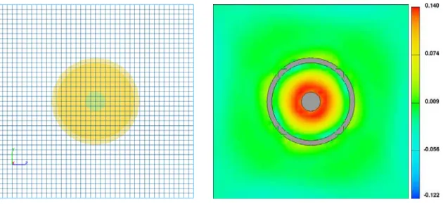
area, the size of an individual mesh cell will be increased, which means the number of cells in a unit of area will be decreased, and the accuracy of measurements and the quantity of result images will be decreased as well. The mesh cell for this simulation is determined as a 1cm cubic. For example, the model has 2cm thickness that covers two mesh cells. The structure has to cover at least one mesh cell so that the software can recognize it during the simulation. A straight structure can be easily covered by one mesh cell, but a round structure may not be fully covered. As a result, the round structure may contain a tiny hole, and the result will be influenced. Figure 5 indicates a crossing view of a rotating impeller in a pipe. The pipe has 1cm thickness and some area is not entirely covered by a mesh cell, and thus the water in pipe is leaking to the outside, which is shown in the image at right hand side of Figure 1. The mesh cell is fixed at a certain location, and the fluid particles will pass through this cell during the simulation. One mesh cell will give the same measurement. In order to measure the data in the middle of two adjacent cells, the value from these cells has to be averaged. Researching the flow area can be used to analyze the collected data at the mesh cells in this area, which proves that the software has a Eulerian method approach.

Figure 1: Leaking water in a pipe

In addition, the boundary condition must be specified for the purpose of accomplishing a simulation. The boundary is set for each mesh boundary and obstacle surface. The default boundary condition is a symmetry plane which means that the flow can cross the boundary without producing any velocity and turbulence. Moreover, there are seven boundaries installed in Flow 3D. The specified pressure boundary can compute the static pressure by subtracting the dynamic pressure from the stagnation pressure. The stagnation pressure can be calculated by the function of

P+ρU²/2. P is the static pressure and ρU²/2 is the dynamic pressure where ρis fluid density, and U

is the normal velocity of incoming flow. The specified velocity boundary defines the velocity of fluid crossing the boundary. The wall boundary defines the normal velocity to be zero, and sets

(10)

monochromatic waves are regular waves that are periodic and linear. The wave speed c and the

wave frequency ω can be expressed as:

λ π π λ h g c tanh2 2 2 = , λ π λ π ω2 =2 gtanh2 h , T =2πω

λ is the wavelength, h is the water depth and g is gravity. The wave period T is calculated by 2* π * ω.

For the simulation of this project, the wave is generated from the wave boundary and moves towards the outlet boundary. The bottom boundary is defined as the wall boundary that can be considered as a floor that is beneath a water tank. The boundary for water current moving out is defined as a continuative boundary.

3 COMPUTATIONAL PROCEDURES

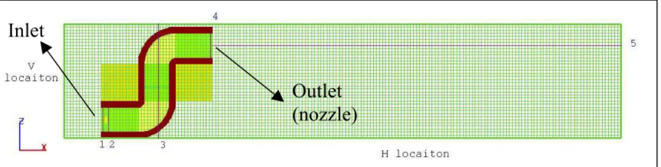
The data is collected at the last second before finishing the numerical simulation. The measurements are obtained from five locations. Figure 2 indicates a cross-sectional view in the middle of an S shape tube, which will be explained after. The model consists of a single inlet and a single outlet, and the outlet part can also be treated as a nozzle. The impeller is installed at the inlet, which is located in between positions 1 and 2 and its hub can be seen in yellow color. The horizontal velocities are measured at locations 1 and 2 in the vertical direction. The vertical velocities are measured on line 3, which covers the domain water depth at the center pipe. The horizontal velocities at location 4 cover the outlet depth. The distributions of the horizontal velocities along the centerline from location 4 to location 5 are measured. This gives the propagation and quality of the current flow that going out of the model outlet over horizontal distance 4 to 5. Each location covers a series of mesh cells that are linearly arranged, and thus the measurements are taken as an array. By surveying the plot of arrays in Excel, the current’s performance generated by different models can be compared. The obtained results over the horizontal location from 4 to 5 can be used as a major comparison parameter for analyzing different models. Different physical configurations of the models and impeller spins are used to study the phenomenon. Single impeller and multiple impellers are used. Wave generation in the domain are discussed. A simple example of the wave-current interaction is shown.

Inlet

Outlet (nozzle)

(11)

4 ANALYSES OF SINGLE IMPELLER MODELS 4.1 Nozzle Analysis

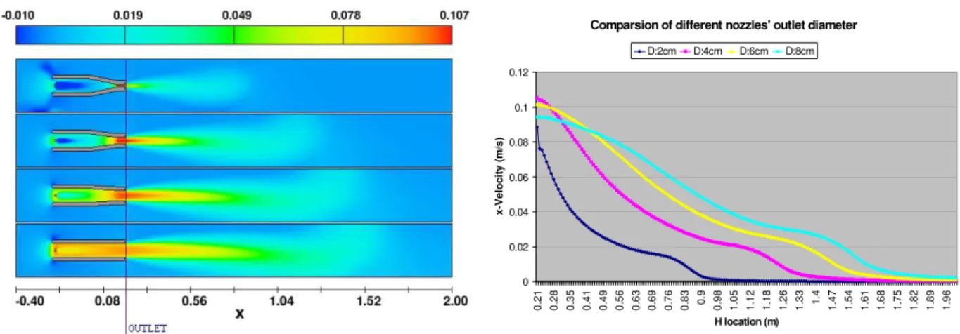
Initially, the nozzle (outlet) of a model is analyzed. The inlet length and diameter is kept constant for all case we tested. We only varied the diameter of the nozzle outlet. The impeller is installed at the inlet of each nozzle. The spin rate of the impeller is set at 50 rad/s, and the impeller diameter, which is the inlet diameter, is taken 8cm, and the selected outlet diameters are 2cm, 4cm, 6cm and 8cm. As shown in the left image of Figure 3, the outlets of four nozzles are placed at the same location, and the colors represent the fluid velocities over horizontal direction. The performance of different nozzles can be obviously obtained by comparing the propagation of the generated currents over horizontal distance. The nozzle with 8cm outlet diameter, which is shown in the bottom image, has the best performance because the generated current can sustain longer than others. Furthermore, the graph shown at right plots the horizontal velocity of current that distributes on the horizontal line from 4 to 5, which is discussed in computational procedures. The horizontal velocity of the current generated by an 8 cm outlet diameter drops smoother and sustains longer than others. Therefore, the nozzle that has the same diameter between outlet and inlet, which can be considered a pipe or a tube, is selected for this project.

Comparsion of different nozzles' outlet diameter

0 0.02 0.04 0.06 0.08 0.1 0.12 0. 21 0. 28 0. 35 0. 41 0. 49 0. 56 0. 63 0. 69 0. 76 0. 83 0.9 _0.98 1. 05 1. 12 1. 18 1. 26 1. 33 1.4 _1.47 1. 54 1. 61 1. 68 1. 75 1. 82 1. 89 1. 96 H location (m) x-Velo ci ty ( m /s ) D:2cm D:4cm D:6cm D:8cm

Figure 3: Result image and current velocity plot for nozzle outlet diameter changing

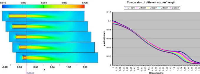
In order to study the effect of the nozzle length we varied its lengths from 10cm to 50cm, and the observations are taken al every 10cm. Figure 4 shows a image and a plot of the current velocity. The image shows the outlet of different nozzles at the same starting line and the colors distributions represent the velocity on horizontal direction. The plot shows the horizontal velocity of water current on the computational location (4-5). It can be seen in the plot that a nozzle that has the shortest length that we considered here demonstrates the best performance in current propagation in terms of magnitude and propagation distance.

(12)

Comparsion of different nozzles' length 0 0.02 0.04 0.06 0.08 0.1 0.12 0 0.08 0.15 0.22 0.29 0.36 0.43 0.5 0.57 0.63 0.7 0.77 0.85 0.92 0.99 1.05 1.13 1.2 1.27 1.34 1.41 1.48 1.55 1.62 1.68 H location (m) x-V e locit y ( m /s) L:10cm L:20cm L:30cm L:40cm L:50cm

Figure 4: Result image and current velocity plot for nozzle length changing

4.2 Model Shape Selection

Using an outlet that has the same diameter as the inlet, three models are tested for analyzing the performance of water current influenced by different kinds of model shape. In Figure 5, the U shape model, which is shown at the left, has the inlet (impeller) and outlet at the same side. The image at the right hand side is the S shape model, has its inlet (impeller) and outlet on the opposite sides. The image in the middle is the LL shape model whose inlet (impeller) is perpendicular to its outlet. In this test the height of the models, total time of simulations and the spin rate are kept constant in all cases.

Figure 5: U shape, LL shape and S shape models

The image shown at the left of Figure 6 indicates that the currents from the above three different models dissipate almost at the same location, so it is hard to compare the performance of water current just from the visualization. For better understanding, the graph shown at right shows the horizontal velocities of currents on the horizontal location (4-5). The S shape and U shape models can generate water current, which sustains for a long distance but the horizontal velocity of the current drops suddenly. The water current generated by LL shape model has the best performance because the current smoothly diffuses which means that the energy of the current can maintain long distance. Consequently, the LL shape model is used for analyzing single impeller study.

(13)

Comparsion of different model shapes 0 0.02 0.04 0.06 0.08 0.1 0.12 0.14 0. 19 0. 25 0. 31 0. 37 0. 43 0. 49 0. 55 0. 61 0. 67 0. 73 0. 78 0. 85 0.9 _0.97 1. 03 1. 09 1. 15 1. 21 1. 27 1. 33 1. 39 1. 45 H location (m) x-Vel o ci ty ( m /s )

U shape LL shape S shape

Figure 6: Result image and current velocity plot for different shapes

4.3 Model Height Research

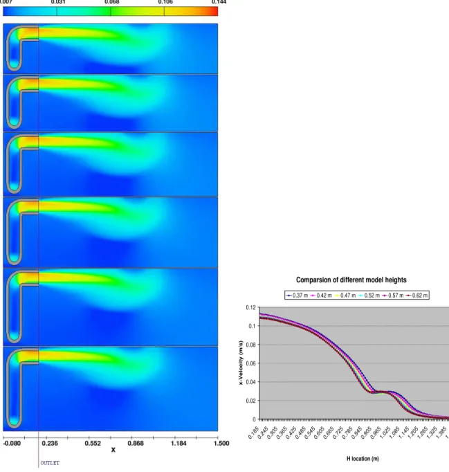
In addition, the height of a model also affects the test result. The energy of generated water current will be decreased due to the friction between fluid and object surface. If the model’s height is increased, which has a large contact area between fluid and object surface, the friction energy loss will be increased. Furthermore, if the outlet position is installed at a high location, the potential energy of the current will be increased because of gravity so that the direction of current will be easily moved downwards. The selected LL shape model is used to analyze the performance affected by its height. The model’s height is increased every 5cm, and the impeller spin rate and the simulation time are remained constant. As shown in the result image and current velocity plot in Figure 7, the different performance of increasing model’s height is extraordinary small, and the water current generated by a model with the lowest height drops slower and sustains longer than other models.

(14)

Comparsion of different model heights 0 0.02 0.04 0.06 0.08 0.1 0.12 0.18 5 0.24 5 0.30 5 0.36 5 0.42 5 0.48 5 0.54 5 0.60 5 0.66 5 0.72 5 0.78 5 0.84 5 0.90 5 0.96 5 1.02 5 1.08 5 1.14 5 1.20 5 1.26 5 1.32 5 1.38 5 1.44 5 H location (m) x -Ve lo cit y ( m /s) 0.37 m 0.42 m 0.47 m 0.52 m 0.57 m 0.62 m

Figure 7: Result image and current velocity plot for different models’ height

4.4 Analysis of Impeller Spin Rate

An impeller is the source of momentum to generate water current, and the impeller is activated by its spin rate. The unit of spin rate is radian per second (rad/s) and also can be converted into revolutions per minute (RPM) by following equation:

2

1 /

60

RPM = π rad s

In order to study the current velocity influenced by impeller spin rate, the height of LL shape model is fixed and the impeller spin rate is varied from 50 rad/s to 250 rad/s, and the measurements are taken at every 50 rad/s. As observed in Figure 8, the model will have a better performance as the spin rate increases.

(15)

Comparsion of different impellers' spin rate 0 0.02 0.04 0.06 0.08 0.1 0.12 0.14 0.16 0.18 0.2 0. 19 0. 26 0. 35 0. 43 0. 51 0. 58 0. 67 0. 75 0. 82 0.9 0. 99 1. 07 1. 15 1. 23 1.3 1. 39 1. 47 1. 55 1. 63 1. 71 1. 79 1. 87 1. 95 H location (m) x-V e locit y ( m /s )

50 rad/s 100 rad/s 150 rad/s 200 rad/s 250 rad/s

Figure 8: Result image and current velocity plot for different impeller spin rate

4.5 Single Impeller Model with Multiple Outlets

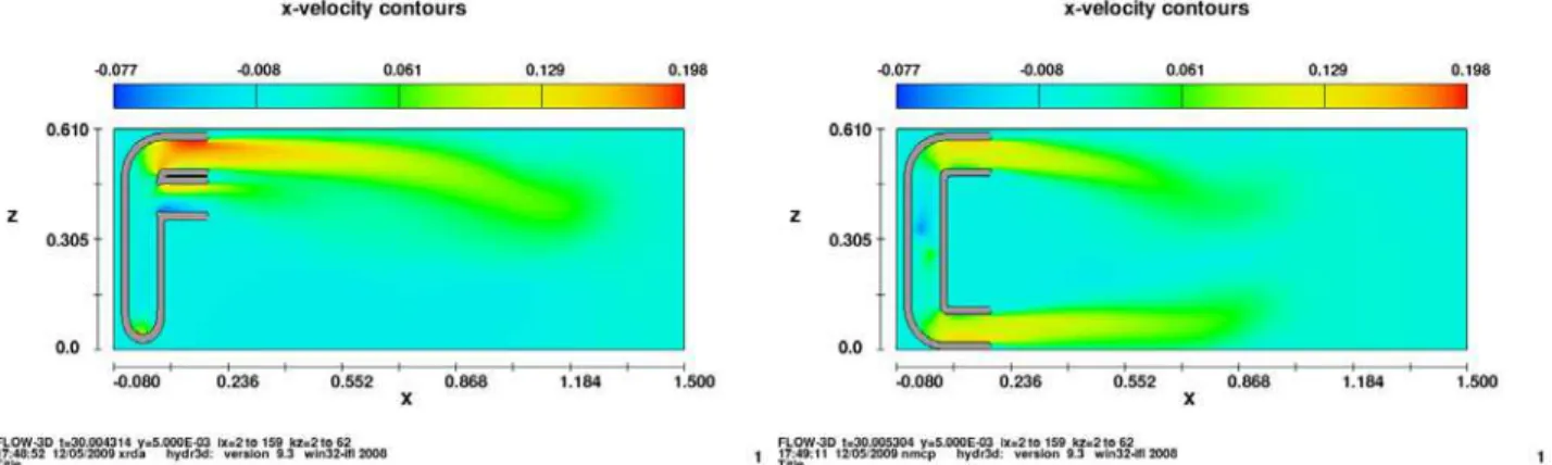
The single impeller models that contain more than one outlet are designed and analyzed to study the property of the generated water currents. Two LL shape models with the same height are used to study the models’ performance. One model has one inlet and two outlets one above another and, the other one has one inlet at the middle and two outlets are at the top and at the bottom. Figure 9 expresses the results.

(16)

Figure 9: Result images of single impeller model with two outlets

5 ANALYSES OF MULTIPLE IMPELLERS MODELS

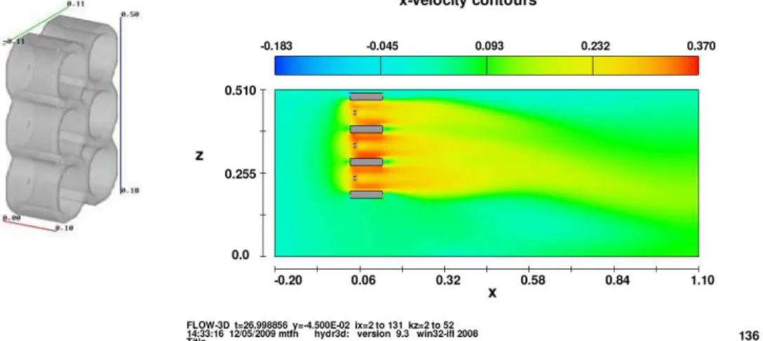
It is observed from the previous chapters that a single inlet and multiple outlet models don’t seem to produce quality currents over a certain depth. To develop a model that can generate currents over a depth, a model with multiple impellers and multiple outlets is chosen. In terms of nozzle and impeller studies, the model combines many inlets and outlets together, which have the same diameters. The nozzles have a length of 10cm, and the impellers are installed at each nozzle’s inlet. The spin rate of each impeller is taken as 300 rad/s, and the simulation time is 30 seconds. Two multiple impeller models are created to generate water currents that cover a certain water depth. As shown in Figure 10, a multiple impeller model with 10 nozzles, and the image at the right hand side represents the water currents that cover the whole water depth. Figure 11 expresses a multiple impeller with 6 nozzles, and the generated water currents only cover the area near the water surface.

(17)

Figure 11: Result images of 6 impellers’ model

5.1 An Application of Wave-current Interaction

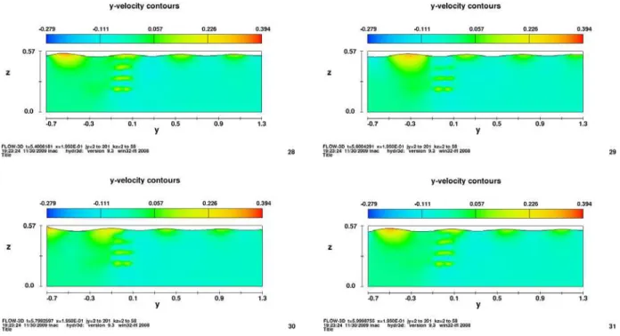
After the model is designed to generate currents that cover a certain water depth, a monochromatic wave is utilized to study a wave-current interaction. The model is placed in a 2m X 1.3m mesh block, which consists of more than 1.5 million cells. The total simulation time is 15 seconds, and it took 2 days runtime. The wave amplitude is 2cm and the wavelength is 50cm, and the impeller spin rate is set at 1000 rad/s. Figure 12 and Figure 13 show the process of wave-current interaction for the 10 and 6 outlet models. The distributed colors are the velocities on the y-axis shown in horizontal direction in these images. Waves are coming from left to right on the images, and water currents are pushing into the page the x-axis, toward the reader. Consequently, the direction of the wave is perpendicular to the current. It is observed that wave height on the right hand side on the figures is suppressed due to current action.

(18)

Figure 13: Result images of wave-current interaction (10 outlets)

6 CONCLUSIONS

In order to develop and test a portable stand-alone current generator that can generate quality currents for OEB, a Flow 3D CFD code can be used to study a current-related model. Flow 3D is utilized to study the concept of single and multiple impeller type current generators. The single impeller model can be installed with a single outlet or multiple outlets. A multiple impellers model has multiple outlets installed. After different studies it is perceived that a current generator with multiple impellers and multiple outlets can provide better currents that cover a certain water depth. It is observed that water currents can reduce the wave heights of an incoming wave field.

(19)

REFERENCES

[1] FLOW-3D, “User Manual, Version 9.3”, FLOW Science Inc, 2008

[2] M. Hasanat Zaman, “Suppression of Ocean Waves by Uniform Forced Currents”, 27th International Conference on Offshore Mechanics and Arctic Engineering, June 15-20, 2008

(20)

APPENDICES

CFD CODE OF A NOZZLE WITH 6CM OUTLET DIAMETER

&xput

remark='Units are SI',

nmat=1, remark='One material', gz=-9.81, remark='Define gravity',

ipdis=1, remark='Hydrostatic pressure z-axis',

ifvisc=2, remark='Viscosity coefficient-function of strain rate', iwsh=1, remark='Wall shear stress',

ifvis=3, remark='two-equation (k-e) turbulence model', itb=1, remark='Free surface or sharp interface', icav=1, remark='Activate cavitation',

delt=0.01, remark='Initial time-step size', twfin=60, remark='Time to end calculation', pltdt=1, remark='Time interval',

/ &limits

remark='Output Window, Iteration Limits', itmax=1000,

itflmx=150, /

&props

rhof=1000., rhofs=917., thexf1=0.00018, cv1=4182., cvs1=2100., pofl1=0., thc1=0.597, thcs1=2.215, clht1=3.35e+05, ts1=273., tl1=273., tniyam=-1., tsdrg=1., mu1=0.001, muc00=0., muc0=1., muc1=0.001, muc2=0., muc3=0., mutmp1=0., mutmp2=0., mutmp3=1., muthk=0., muthn0=0., muthn1=0., cangle=90., sigma=0.073, csigma=0., rf2=2.87e+06, tmelt=0., teut=0., ceut=0.,

cexf1=0., cstar=0., dratio=0., pcoef=0., fluid1='Water at 20 C', units='SI', / &scalar / &bcdata wb=2, wr=3, wl=3, wt=5, pbct(1,6)=0.0, / &mesh nxcelt=240, px(1)=-0.4, px(2)=2, nycelt=30, py(1)=-0.15, py(2)=0.15, nzcelt=30, pz(1)=-0.15, pz(2)=0.15, / &obs avrck=-2.1, nobs=3, remark='impeller', iob(3)=3,

(21)

ifob(3)=2,

zl(3)=0., zh(3)=0.01, ral(3)=0.01, rah(3)=0.04,

icpy(1)=3, croty(1)=90., ctrnx(1)=-0.19,

ospin(1,3)=50, oadrg(3)=0.8, obdrg(3)=0.8, remark='hub', iob(2)=2, zl(2)=0., zh(2)=0.01, rah(2)=0.01, trnx(2)=-0.19, roty(2)=90., remark='component', iob(1)=1, zl(1)=-0.1, zh(1)=0.1, ral(1)=0.04, rah(1)=0.06, roty(1)=90., trnx(1)=-0.1, iob(4)=1, zl(4)=0., zh(4)=0.90, roty(4)=-90., trnx(4)=0.9, coneh(4)=3.814074834, iob(5)=1, ioh(5)=0, zl(5)=0., zh(5)=0.6, roty(5)=-90., trnx(5)=0.6, coneh(5)=3.814074834, iob(6)=1, ioh(6)=0, xl(6)=0., xh(6)=0.8, yl(6)=-0.06, yh(6)=0.06, zl(6)=-0.06, zh(6)=0.06, trnx(6)=0.15,

ifrco(2)=1, ifrco(3)=1, ifrco(1)=1, iob(7)=1, zl(7)=0., zh(7)=0.05, ral(7)=0.03, rah(7)=0.05, roty(7)=90., trnx(7)=0.15, / &fl fioh(1)=1, nfls=1, fxl(1)=-0.4,fzh(1)=0.15, / &bf / &temp / &motn / &grafic / &HEADER

(22)

RESULTANT IMAGES AND FLOW VELOCITY PLOTS OF ANALYZING NOZZLE’S OUTLET DIAMETER

(23)

Comparsion of different nozzles' outlet diameter (4-5) 0 0.02 0.04 0.06 0.08 0.1 0.12 0.21 0.28 0.35 0.41 0.49 0.56 0.63 0.69 0.76 0.83 0.9 0.98 1.05 1.12 1.18 1.26 1.33 1.4 1.47 1.54 1.61 1.68 1.75 1.82 1.89 1.96 H location (m) x-V e lo ci ty ( m /s ) D:2cm D:4cm D:6cm D:8cm

Horizontal velocity before impeller (1)

-0.04 -0.03 -0.02 -0.01 0 0.01 0.02 0.03 0.04 -0.08 -0.06 -0.04 -0.02 0 0.02 0.04 0.06 0.08 0.1 0.12 x-Velocity (m/s) V l o c a ti o n (m ) D:2cm D:4cm D:6cm D:8cm

Horizontal velocity after impeller (2)

-0.04 -0.03 -0.02 -0.01 0 0.01 0.02 0.03 0.04 -0.08 -0.06 -0.04 -0.02 0 0.02 0.04 0.06 0.08 0.1 0.12 x-Velocity (m/s) V lo c a tio n ( m ) D:2cm D:4cm D:6cm D:8cm

Horizontal velocity at outlet (4)

-0.04 -0.03 -0.02 -0.01 0 0.01 0.02 0.03 0.04 V l o ca ti o n (m ) D:2cm D:4cm D:6cm D:8cm

(24)

RESULTANT IMAGES AND FLOW VELOCITY PLOTS OF ANALYZING NOZZLE’S LENGTH

(25)

Comparsion of different nozzles' length (4-5) 0 0.02 0.04 0.06 0.08 0.1 0.12 0 0. 08 0. 15 0. 22 0. 29 0. 36 0. 43 0.5 _0.57 0. 63 0.7 _0.77 0. 85 0. 92 0. 99 1. 05 1. 13 1.2 _1.27 1. 34 1. 41 1. 48 1. 55 1. 62 1. 68 H location (m) x-V eloc ity (m /s ) L:10cm L:20cm L:30cm L:40cm L:50cm

-0.04 -0.03 -0.02 -0.01 0 0.01 0.02 0.03 0.04 0.07 0.08 0.09 0.1 0.11 0.12 0.13 x-Velocity (m/s) V l o ca ti o n (m ) L:10cm L:20cm L:30cm L:40cm L:50cm

(26)

CFD CODE OF THE LL SHAPE MODEL

&xput

delt=0.01, remark='Initial time-step size', twfin=30., remark='Time to end calculation', pltdt=1., remark='Time interval',

/ &limits

itflmx=150, /

&props

cexf1=0., cstar=0., dratio=0., pcoef=0., fluid1='Water at 20 C', units='SI', / &scalar / &bcdata wb=2, wt=5, wr=3, wl=3, pbct(1,6)=0.0, / &mesh px(1)=-0.08, px(2)=1.5, py(1)=-0.3, py(2)=0.08, pz(1)=0., pz(2)=0.37, size=0.01, obs avrck=-2.1, nobs=4, remark= 'impeller', iob(3)=3, ivrt(3)=1, ifob(3)=2, ral(3)=0.01, rah(3)=0.04, / &

(27)

icpy(1)=3, croty(1)=-90.,ctrnz(1)=0.06, crotz(1)=90., ospin(1,3)=100., oadrg(3)=0.8, obdrg(3)=-0.8,

remark = 'component tube',

=0.01, 2)=0.06, rotz(2)=90., , iob(8)=1, 0., crxy(8)=-0.12, rny(8)=-0.06, ., trny(9)=-0.06, yl(10)=-0.06, yh(10)=0.06, =0., zh(10)=0.24, trnx(10)=0., rotz(10)=90., trny(10)=-0.06, 1, (11)=0.12, h(11)=0.06, 11)=0.24, 1)=0.0, rotz(11)=90., trny(11)=-0.06, urve', 4)=-0.12, cy2(4)=1.0, cz2(4)=1.0, trnx(4)=0.06, trnz(4)=0.24, cc(5)=0.002, crxy(5)=-0.12, iob(12)=4, ral(12)=0.04, rah(12)=0.06, zl(12)=0.06, zh(12)=0.18, roty(12)=90., trnz(12)=0.3, iob(13)=4, ral(13)=0.04, rah(13)=0.06, zl(13)=0.06, zh(13)=0.18, roty(13)=-90., trnz(13)=0.06, rotz(13)=90., iob(14)=4, ral(14)=0.04, rah(14)=0.06, zl(14)=0.12, zh(14)=0.24, remark = 'hub', iob(2)=2, rah(2) zl(2)=0.16, zh(2)=0.17, roty(2)=-90., trnz( m curve' remark ='botto cc(8)= cx2(8)=1.0, cy2(8)=1.0, cz2(8)=1.0, 90., t rotx(8)=90., trnx(8)=0., trnz(8)=0.12, rotz(8)= iob(9)=1, ioh(9)=0, cc(9)=0.002, crxy(9)=-0.12, cx2(9)=1.0, cy2(9)=1.0, cz2(9)=1.0, rotx(9)=90., trnx(9)=0., trnz(9)=0.12, rotz(9)=90 iob(10)=1, ioh(10)=0, xl(10)=-0.12, xh(10)=0., zl(10) iob(11)= ioh(11)=0, xl(11)=-0.12, xh yl(11)=-0.06, y zl(11)=0.12, zh( trnx(1 remark ='top c iob(4)=1, cc(4)=0., crxy( cx2(4)=1.0, 0., rotx(4)=9 iob(5)=1, ioh(5)=0,

(28)

xl(7)=0., xh(7)=0.12, yl(7)=-0.06, yh(7)=0.06, zl(7)=0.12, zh(7)=0.36, trnx(7)=0.06, =1, ifrco(4)=1, 37, ifrco(2)=1, ifrco(3)=1, ifrco(1) / &fl fioh(1)=1, nfls=1, fxl(1)=-0.08,fzh(1)=0. / &bf / &temp / &motn / &grafic / &HEADER PROJECT='8cmLL', / &parts /

(29)

S AND FLOW VELOCITY PLOTS OF SHAPE SELECTION RESULTANT IMAGE

(30)

Comparsion of different model shapes (4-5) 0 0.02 0.04 0.06 0.08 0.1 0.12 0.14 0. 19 0. 25 0. 31 0. 37 0. 43 0. 49 0. 55 0. 61 0. 67 0. 73 0. 78 0. 85 0.9 _0.97 1. 03 1. 09 1. 15 1. 21 1. 27 1. 33 1. 39 1. 45 H location (m) x-V el oci ty ( m /s )

0.02 0.03 0.04 0.05 0.06 0.07 0.08 0.09 0.1 0.05 0.06 0.07 0.08 0.09 0.1 0.11 0.12 0.13 0.14 x-Velocity (m/s) V l o ca ti o n (m )

0 0.01 0.02 0.03 0.04 0.05 0.06 0.07 0.08 0.09 0.1 0.05 0.06 0.07 0.08 0.09 0.1 0.11 0.12 0.13 0.14 x-Velocity (m/s) V l o ca ti o n (m )

Vertical velocity at the center of middle pipe (3)

0 0.05 0.1 0.15 0.2 0.25 0.3 0.35 0.4 -0.02 0 0.02 0.04 0.06 0.08 0.1 0.12 0.14 z-Velocity (m/s) V l o ca ti o n (m )

(31)

RESULTANT IMAGES AND FLOW VELOC TY PLOTS OF RESEARCING MODEL HEIGHT

(32)

(33)

Comparsion of different model heights (4-5) 0 0.02 0.04 0.06 0.08 0.1 0.12 0.18 5 0.24 5 0.30 5 0.36 5 0.42 5 0.48 5 0.54 5 0.60 5 0.66 5 0.72 5 0.78 5 0.84 5 0.90 5 0.96 5 1.02 5 1.08 5 1.14 5 1.20 5 1.26 5 1.32 5 1.38 5 1.44 5 H location (m) x-V e lo cit y ( m /s) 0.37 m 0.42 m 0.47 m 0.52 m 0.57 m 0.62 m

0.02 0.03 0.04 0.05 0.06 0.07 0.08 0.09 0.1 0.06 0.07 0.08 0.09 0.1 0.11 0.12 0.13 0.14 x-Velocity (m/s) V l o ca ti o n (m ) 0.37 m 0.42 m 0.47 m 0.52 m 0.57 m 0.62 m

0 0.01 0.02 0.03 0.04 0.05 0.06 0.07 0.08 0.09 0.1 0.06 0.07 0.08 0.09 0.1 0.11 0.12 0.13 x-Velocity (m/s) V l o ca ti o n (m ) 0.37 m 0.42 m 0.47 m 0.52 m 0.57 m 0.62 m

0.26 0.27 0.28 0.29 0.3 0.31 0.32 0.33 0.34 0.06 0.07 0.08 0.09 0.1 0.11 0.12 0.13 0.14 x_velocity (m/s) V l o ca ti o n (m ) 0.37 m 0.42 m 0.47 m 0.52 m 0.57 m 0.62 m

0 0.1 0.2 0.3 0.4 0.5 0.6 0.7 -0.02 0 0.02 0.04 0.06 0.08 0.1 0.12 0.14 z-Velocity (m/s) V l o ca ti o n (m ) 0.37 m 0.42 m 0.47 m 0.52 m 0.57 m 0.62 m

(34)

RESULTANT IMAGES AND FLOW VELOCITY PLOTS OF ANALYZING IMPELLER SPIN RATE

(35)

(36)

Comparsion of different impellers' spin rate (4-5) 0 0.02 0.04 0.06 0.08 0.1 0.12 0.14 0.16 0.18 0.2 0. 19 0. 26 0. 35 0. 43 0. 51 0. 58 0. 67 0. 75 0. 82 0.9 _0.99 1. 07 1. 15 1. 23 1.3 _1.39 1. 47 1. 55 1. 63 1. 71 1. 79 1. 87 1. 95 H location (m) x-V e lo ci ty ( m /s )

0 0.01 0.02 0.03 0.04 0.05 0.06 0.07 0.08 0.09 0.1 0.04 0.06 0.08 0.1 0.12 0.14 0.16 0.18 0.2 0.22 x-Velocity (m/s) V l o ca ti o n (m )

0 0.1 0.2 0.3 0.4 0.5 0.6 0.7 -0.03 0.02 0.07 0.12 0.17 0.22 z-Velocity (m/s) V l o ca ti o n (m )

(37)

CFD CODE OF MULTIPLE IMPELLERS MODELS WITH 10 OUTLETS

&xput

delt=0.01, remark='Initial time-step size', twfin=30., remark='Time to end calculation', pltdt=0.5, remark='Time interval',

/ &limits

itflmx=150, /

&props

cexf1=0., cstar=0., dratio=0., pcoef=0., fluid1='Water at 20 C', units='SI', / &scalar / &bcdata wb=2, wt=5, wr=3, wl=3, pbct(1,6)=0.0, / &mesh px(1)=-0.3, px(2)=1.1, py(1)=-0.15, py(2)=0.15, pz(1)=0., pz(2)=0.53, size=0.01,

(38)

ral(1)=0.01, rah(1)=0.04, zl(1)=0.04, zh(1)=0.05, icpy(1)=1, croty(1)=90.,ctrnz(1)=0.06,ctrny(1)=0.05, g(1)=0.8, obdrg(1)=0.8, )=3, croty(3)=90.,ctrnz(3)=0.26,ctrny(3)=0.05, .8, ifob(4)=2, =0.01, rah(4)=0.04, , trny(5)=0.05, )=0.8, iob(6)=6, 1, ifob(6)=2, 0.01, rah(6)=0.04, zh(6)=0.05, y(6)=90.,ctrnz(6)=0.06,ctrny(6)=-0.05, 1,6)=300., oadrg(6)=0.8, obdrg(6)=0.8, ivrt(7)=1, )=2, , rah(7)=0.04, zh(7)=0.05, oty(7)=90.,ctrnz(7)=0.16,ctrny(7)=-0.05, 00., oadrg(7)=0.8, obdrg(7)=0.8, 1, rah(8)=0.04, )=0.04, zh(8)=0.05, y(8)=90.,ctrnz(8)=0.26,ctrny(8)=-0.05, =300., oadrg(8)=0.8, obdrg(8)=0.8, rah(9)=0.04, ospin(1,1)=300., oadr iob(2)=2, ivrt(2)=1, ifob(2)=2, ral(2)=0.01, rah(2)=0.04, zl(2)=0.04, zh(2)=0.05, icpy(2)=2, croty(2)=90.,ctrnz(2)=0.16,ctrny(2)=0.05, ospin(1,2)=300., oadrg(2)=0.8, obdrg(2)=0.8, iob(3)=3, ivrt(3)=1, ifob(3)=2, ral(3)=0.01, rah(3)=0.04, zl(3)=0.04, zh(3)=0.05, icpy(3

ospin(1,3)=300., oadrg(3)=0.8, obdrg(3)=0 iob(4)=4, ivrt(4)=1, ral(4) zl(4)=0.04, zh(4)=0.05, 0.05 icpy(4)=4, croty(4)=90.,ctrnz(4)=0.36,ctrny(4)= ospin(1,4)=300., oadrg(4)=0.8, obdrg(4)=0.8, iob(5)=5, ivrt(5)=1, ifob(5)=2, ral(5)=0.01, rah(5)=0.04, zl(5)=0.04, zh(5)=0.05, icpy(5)=5, croty(5)=90.,ctrnz(5)=0.46,c drg(5 ospin(1,5)=300., oadrg(5)=0.8, ob ivrt(6)= ral(6)= zl(6)=0.04, 6, crot icpy(6)= ospin( iob(7)=7, ifob(7 ral(7)=0.01 , zl(7)=0.04 icpy(7)=7, cr ospin(1,7)=3 iob(8)=8, ivrt(8)=1, ifob(8)=2, ral(8)=0.0 zl(8 icpy(8)=8, crot ospin(1,8) iob(9)=9, ivrt(9)=1, ifob(9)=2, ral(9)=0.01,

(39)

ospin(1,9)=300., oadrg(9)=0.8, obdrg(9)=0.8, 01, rah(10)=0.04, zh(10)=0.05, 0, croty(10)=90.,ctrnz(10)=0.46,ctrny(10)=-0.05, .8, obdrg(10)=0.8, 3, zh(41)=0.13, 0., trnz(41)=0.06, trny(41)=0.05, 4, rah(43)=0.06, zh(43)=0.13, 0., trnz(43)=0.26, trny(43)=0.05, , 4, rah(45)=0.06, zh(45)=0.13, trny(45)=0.05, 0., trnz(47)=0.06, trny(47)=-0.05, 4, rah(48)=0.06, trny(48)=-0.05, 3, zh(49)=0.13, 0., trnz(49)=0.26, trny(49)=-0.05, 4, rah(51)=0.06, zh(51)=0.13, 0., trnz(51)=0.46, trny(51)=-0.05, iob(10)=10, ivrt(10)=1, ifob(10)=2, ral(10)=0. zl(10)=0.04, icpy(10)=1 ospin(1,10)=300., oadrg(10)=0 remark='outlet tube', iob(41)=11, ral(41)=0.04, rah(41)=0.06, zl(41)=0.0 roty(41)=9 iob(42)=11, ral(42)=0.04, rah(42)=0.06, zl(42)=0.03, zh(42)=0.13, roty(42)=90., trnz(42)=0.16, trny(42)=0.05, iob(43)=11, ral(43)=0.0 zl(43)=0.03, roty(43)=9 iob(44)=11, ral(44)=0.04, rah(44)=0.06, zl(44)=0.03, zh(44)=0.13, roty(44)=90., trnz(44)=0.36, trny(44)=0.05, iob(45)=11 ral(45)=0.0 zl(45)=0.03, roty(45)=90., trnz(45)=0.46, iob(47)=11, ral(47)=0.04, rah(47)=0.06, zl(47)=0.03, zh(47)=0.13, roty(47)=9 iob(48)=11, ral(48)=0.0 zl(48)=0.03, zh(48)=0.13, roty(48)=90., trnz(48)=0.16, iob(49)=11, ral(49)=0.04, rah(49)=0.06, zl(49)=0.0 roty(49)=9 iob(50)=11, ral(50)=0.04, rah(50)=0.06, zl(50)=0.03, zh(50)=0.13, roty(50)=90., trnz(50)=0.36, trny(50)=-0.05, iob(51)=11, ral(51)=0.0 zl(51)=0.03, roty(51)=9

(40)

rah(63)=0.01, zl(63)=0.04, zh(63)=0.05, ., trnz(63)=0.26, trny(63)=0.05, , zh(65)=0.05, trny(65)=0.05, , zh(67)=0.05, trny(67)=-0.05, , zh(68)=0.05, trny(68)=-0.05, , zh(69)=0.05, trny(69)=-0.05, , zh(70)=0.05, trny(70)=-0.05, , zh(71)=0.05, trny(71)=-0.05, roty(63)=90 iob(64)=12, rah(64)=0.01, zl(64)=0.04, zh(64)=0.05, roty(64)=90., trnz(64)=0.36, trny(64)=0.05, iob(65)=12, rah(65)=0.01, zl(65)=0.04 roty(65)=90., trnz(65)=0.46, iob(67)=12, rah(67)=0.01, zl(67)=0.04 roty(67)=90., trnz(67)=0.06, iob(68)=12, rah(68)=0.01, zl(68)=0.04 roty(68)=90., trnz(68)=0.16, iob(69)=12, rah(69)=0.01, zl(69)=0.04 roty(69)=90., trnz(69)=0.26, iob(70)=12, rah(70)=0.01, zl(70)=0.04 roty(70)=90., trnz(70)=0.36, iob(71)=12, rah(71)=0.01, zl(71)=0.04 roty(71)=90., trnz(71)=0.46, remark ='nozzle',

remark ='nozzle outlet tube', / &fl fioh(1)=1, nfls=1, fxl(1)=-0.3,fzh(1)=0.6, / &bf / &temp / &motn / &grafic / &HEADER PROJECT='no nozzle', / &parts /

(41)

F AN APPLOCATION OF WAVE-CURRENT INTERATION

e SI',

ark='One material',

ark='Viscosity coefficient-function of strain rate', ark='Wall shear stress',

odel', e', ark='Activate cavitation',

ark='Initial time-step size',

., 1=0., thc1=0.597, thcs1=2.215, ts1=273., tl1=273., tniyam=-1.,

tmp3=1., muthk=0., muthn0=0., le=90., sigma=0.073, csigma=0.,

SI', alar f=1, p(3,1)=0.02, wavefre(3,1)=0.56590145, (3)=0.55,flhtft(1)=0.55, (4)=1, -0.25, 9, , pz(2)=0.59, CFD CODE O &xput remark='Units ar nmat=1, rem gz=-9.81, remark='Define gravity',

ipdis=1, remark='Hydrostatic pressure z-axis', ifvisc=2, rem

iwsh=1, rem

ifvis=3, remark='two-equation (k-e) turbulence m itb=1, remark='Free surface or sharp interfac icav=1, rem

delt=0.01, rem

twfin=15, remark='Time to end calculation', pltdt=0.2, remark='Time interval',

/ &limits

itflmx=150, /

&props

rhof=1000., rhofs=917., thexf1=0.00018, cv1=4182 cvs1=2100., pofl

clht1=3.35e+05,

tsdrg=1., mu1=0.001, muc00=0., muc0=1., muc1=0.001, muc2=0., muc3=0., mutmp1=0., mutmp2=0., mu

muthn1=0., cang

rf2=2.87e+06, tmelt=0., teut=0., ceut=0., cexf1=0., cstar=0., dratio=0., pcoef=0., fluid1='Water at 20 C', units=' / &sc / &bcdata wf=10, wbk=8, wb=2, wr=3, iwave waveam waveh iobctp / &mesh px(1)= px(2)=0. py(1)=-0.7 py(2)=1.3, pz(1)=0.,

(42)

ifob(1)=2, ral(1)=0.01, rah(1)=0.04, zl(1)=0.04, zh(1)=0.05, 0.,ctrnz(1)=0.06,ctrny(1)=0.05, drg(1)=0.8, 5, 0.04, zh(3)=0.05, (3)=0.05, drg(3)=0.8, obdrg(3)=0.8, ivrt(4)=1, )=2, 0.05, rny(5)=0.05, ospin(1,5)=1000., oadrg(5)=0.8, obdrg(5)=0.8,

6, ivrt(6)=1, 2, -0.05, )=2, rah(7)=0.04, , zh(7)=0.05, croty(7)=90.,ctrnz(7)=0.16,ctrny(7)=-0.05, 00., oadrg(7)=0.8, obdrg(7)=0.8, ral(8)=0.01, rah(8)=0.04, )=0.04, zh(8)=0.05, y(8)=90.,ctrnz(8)=0.26,ctrny(8)=-0.05, 00., oadrg(8)=0.8, obdrg(8)=0.8, icpy(1)=1, croty(1)=9 ospin(1,1)=1000., oadrg(1)=0.8, ob iob(2)=2, ivrt(2)=1, ifob(2)=2, ral(2)=0.01, rah(2)=0.04, zl(2)=0.04, zh(2)=0.05, icpy(2)=2, croty(2)=90.,ctrnz(2)=0.16,ctrny(2)=0.0 )=0.8, ospin(1,2)=1000., oadrg(2)=0.8, obdrg(2 iob(3)=3, ivrt(3)=1, ifob(3)=2, ral(3)=0.01, rah(3)=0.04, zl(3)= icpy(3)=3, croty(3)=90.,ctrnz(3)=0.26,ctrny ospin(1,3)=1000., oa iob(4)=4, ifob(4 ral(4)=0.01, rah(4)=0.04, zl(4)=0.04, zh(4)=0.05, icpy(4)=4, croty(4)=90.,ctrnz(4)=0.36,ctrny(4)= 0.8, ospin(1,4)=1000., oadrg(4)=0.8, obdrg(4)= iob(5)=5, ivrt(5)=1, ifob(5)=2, ral(5)=0.01, rah(5)=0.04, zl(5)=0.04, zh(5)=0.05, 0.46,ct icpy(5)=5, croty(5)=90.,ctrnz(5)= iob(6)= ifob(6)= ral(6)=0.01, rah(6)=0.04, zh(6)=0.05, zl(6)=0.04, icpy(6)=6, croty(6)=90.,ctrnz(6)=0.06,ctrny(6)= 8, obdrg(6)=0.8, ospin(1,6)=1000., oadrg(6)=0. iob(7)=7, ivrt(7)=1, ifob(7 ral(7)=0.01, zl(7)=0.04 icpy(7)=7, ospin(1,7)=10 iob(8)=8, ivrt(8)=1, ifob(8)=2, zl(8 icpy(8)=8, crot =10 ospin(1,8) iob(9)=9, ivrt(9)=1, ifob(9)=2,

(43)

icpy(9)=9, croty(9)=90.,ctrnz(9)=0.36,ctrny(9)=-0.05, , obdrg(9)=0.8, 01, rah(10)=0.04, zh(10)=0.05, 0, croty(10)=90.,ctrnz(10)=0.46,ctrny(10)=-0.05, 0.8, obdrg(10)=0.8, 3, zh(41)=0.13, 0., trnz(41)=0.06, trny(41)=0.05, 4, rah(43)=0.06, zh(43)=0.13, 0., trnz(43)=0.26, trny(43)=0.05, , 4, rah(45)=0.06, zh(45)=0.13, trny(45)=0.05, 0., trnz(47)=0.06, trny(47)=-0.05, 4, rah(48)=0.06, trny(48)=-0.05, 3, zh(49)=0.13, 0., trnz(49)=0.26, trny(49)=-0.05, 4, rah(51)=0.06, zh(51)=0.13, ospin(1,9)=1000., oadrg(9)=0.8 iob(10)=10, ivrt(10)=1, ifob(10)=2, ral(10)=0. zl(10)=0.04, icpy(10)=1 ospin(1,10)=1000., oadrg(10)= remark='outlet tube', iob(41)=11, ral(41)=0.04, rah(41)=0.06, zl(41)=0.0 roty(41)=9 iob(42)=11, ral(42)=0.04, rah(42)=0.06, zl(42)=0.03, zh(42)=0.13, roty(42)=90., trnz(42)=0.16, trny(42)=0.05, iob(43)=11, ral(43)=0.0 zl(43)=0.03, roty(43)=9 iob(44)=11, ral(44)=0.04, rah(44)=0.06, zl(44)=0.03, zh(44)=0.13, roty(44)=90., trnz(44)=0.36, trny(44)=0.05, iob(45)=11 ral(45)=0.0 zl(45)=0.03, roty(45)=90., trnz(45)=0.46, iob(47)=11, ral(47)=0.04, rah(47)=0.06, zl(47)=0.03, zh(47)=0.13, roty(47)=9 iob(48)=11, ral(48)=0.0 zl(48)=0.03, zh(48)=0.13, roty(48)=90., trnz(48)=0.16, iob(49)=11, ral(49)=0.04, rah(49)=0.06, zl(49)=0.0 roty(49)=9 iob(50)=11, ral(50)=0.04, rah(50)=0.06, zl(50)=0.03, zh(50)=0.13, roty(50)=90., trnz(50)=0.36, trny(50)=-0.05, iob(51)=11, ral(51)=0.0 zl(51)=0.03,

(44)

zh(63)=0.05, ., trnz(63)=0.26, trny(63)=0.05, , zh(65)=0.05, trny(65)=0.05, , zh(67)=0.05, trny(67)=-0.05, , zh(68)=0.05, trny(68)=-0.05, , zh(69)=0.05, trny(69)=-0.05, , zh(70)=0.05, trny(70)=-0.05, , zh(71)=0.05, trny(71)=-0.05, iob(63)=12, rah(63)=0.01, zl(63)=0.04, roty(63)=90 iob(64)=12, rah(64)=0.01, zl(64)=0.04, zh(64)=0.05, roty(64)=90., trnz(64)=0.36, trny(64)=0.05, iob(65)=12, rah(65)=0.01, zl(65)=0.04 roty(65)=90., trnz(65)=0.46, iob(67)=12, rah(67)=0.01, zl(67)=0.04 roty(67)=90., trnz(67)=0.06, iob(68)=12, rah(68)=0.01, zl(68)=0.04 roty(68)=90., trnz(68)=0.16, iob(69)=12, rah(69)=0.01, zl(69)=0.04 roty(69)=90., trnz(69)=0.26, iob(70)=12, rah(70)=0.01, zl(70)=0.04 roty(70)=90., trnz(70)=0.36, iob(71)=12, rah(71)=0.01, zl(71)=0.04 roty(71)=90., trnz(71)=0.46, remark ='nozzle',

remark ='nozzle outlet tube', / &fl flht=0.55, / &bf / &temp / &motn / &grafic / &HEADER PROJECT='supper_simu', / &parts /